Wage Discrimination Between Jews and Non-Jews in Israel

(1)

Rapport de recherche

Wage Discrimination between

Jews and Non-Jews in Israel

Rédigé par :

Guigui, André

Dirigé par :

Bellou, Andriana

Département de sciences économiques

Faculté des arts et des sciences

(2)

2

I. Introduction

Page 3

II. Historical and Labor Market Context

Page 3

III. Literature Review

Page 6

IV. Theoretical Econometric Model

Page 7

V. Data Specification

Page 10

VI. Econometric Specification

Page 11

VII. Regression Results

Page 11

VIII. Blinder-Oaxaca Decomposition

Page 15

IX. Conclusion

Page 16

Bibliography

Page 18

Appendix I

Page 19

Appendix II

Page 21

(3)

3

I.

Introduction

Israel. The name alone produces strong reactions whatever one’s personal feelings on the subject might be. Despite being historically ancient, it is politically recent. In the short time since its independence it has faced many challenges, from wars, to economic downturns, mass immigration as well as many other difficult situations.

Given the advanced nature of its academic accomplishments, it is hard to believe that the major challenges facing this country, according to an OECD report in 2008, are inequality and poverty. There are many wealthy people, but in contrast there are entire segments of the population that live far below the poverty line. Part of that stems from personal beliefs (the Bedouins, the Heradrim), but part of that inequality comes from discrimination towards other ethnicities, possibly even between some of the different “types” of Jews.

The goal of this report is to present a quantifying measure of the discrimination in Israel using the Blinder-Oaxaca decomposition model. Not only do we intend on measuring the “scale” of discrimination but using data from 3 separate censuses we will try and analyze the trend of “discrimination” in Israel. This type of research is crucial in understanding the mechanism that rule the labor market in the hope of finding an appropriate policy or institutional response.

We will provide an overview of some of the relevant literature on the subject, as well as our chosen theoretical model. We will detail the data used, some of the summary statistics and the results from the regression analysis to see if the real world data coincides with the research and the theory on the subject.

II. Historical and Labor Market Context

In the short time since Israels It has been involved in wars, economic crises, large political change, and all of these external forces have helped shape the mentality of the people and the labor market. It is what leads the Israelis to act the way they do, and according to the experts on the matter, discriminate against different ethnicities, Jewish or not. This section is to show a brief overview of the events that can’t help but impact on the attitudes of workers and hirers.

(4)

4 Israel declared its independence on May 14th 1948 and on May 15th was attacked by neighboring Arab armies (Egypt, Iraq, Transjordan and Syria). Israel fought off the invaders, and on May 11th 1949 was accepted by majority vote as a member of the United Nations. Since then there have been many wars with its neighbors like: 1967, Six Day War; 1973, Yom Kippur War; 1982, Lebanese Invasion; 1986, Palestinian Uprising; 2006, War in Lebanon. In that time there have also been minor uprisings, terrorist attacks by Hezbollah, the Palestinian Liberation Organization (PLO), and surgical military strikes against potential enemies, like the destruction of an Iraqi Nuclear generator in 1987.

There is a clear pattern and it is that almost all of these events involve Arab nations or factions. Only 3 members of the Arab league, Egypt, Jordan and Mauritania maintain diplomatic relations with Israel. Under Israeli law, Lebanon, Syria, Saudi Arabia, Iraq, Iran, Sudan, and Yemen are considered enemy countries. Since the largest minority non-Jewish group in Israel are Arabs it would certainly help account for the discrimination in place.

From an economic point of view, Israel relies heavily on the High-Technology sector, public defense, Academia and some agriculture for its revenue. It is one of the most advanced economies in the region, and was voted most efficient central bank in the world in 2010 for being resistant to economic crisis. That is a far cry from some of turmoil the country faced in its earlier years. In the early 1980’s the country went through a phase of hyperinflation that devalued its currency and endangered its economic health.

As a result of conservative fiscal policy and the implementation of a new currency, the New Israeli Shekel on January 1st 1986, they were able to recover from the crisis. But it is possible some of the remedies enforced at that time have led to the more contemporary problems, such as limited social support, limited access to unemployment benefits, shortened periods of coverage among other cuts. Some of the sacrifices made then no doubt helped contribute to the widespread poverty now affecting the country.

Politically, there have been many changes in leadership and policy over the years. Much of the early years of Israel was based on a “never again” mentality that reflected in a non-compromising,

confrontational approach. Following the wars and the economic turmoil of the 1980’s and 1990’s a new political party proposing peace was elected to power. Partly due to the new immigrants, and the lack of progress from the previous administrations, this new Political party presents a change in public opinion,

(5)

5 and one would think that such a change would be reflected in the attitudes on the labor market. We will discuss this in the analysis section of this report.

From a demographic point of view, Israel has seen some huge changes over the years, and this also has an impact on the actions and attitudes of Israelis. In 1948, at its independence there were

approximately 800,000 citizens. In 1958 thanks mostly to immigration from North African countries that number rose to 2,000,000. Due to larger than average birth rates (compared to other OECD countries) and continued immigration the country reached 4,000,000 in the early 1980’s. After the fall of the Soviet Union and the opening of the borders of the Eastern bloc, many Jews from Russia immigrated and there was a mass migration to Israel in the early 1990’s that brought in around 1,000,000 more citizens. In 2013 it is estimated to be over 8,000,000, nearly 10 times that at its independence a mere 65 years earlier. Immigration accounts for 40% of the Israeli population.

The population is made up of roughly 75% Jews (North African Sefarades, Eastern European Ashkenazy, and Israelis), followed by 21% Arabs (83% Muslim, 8% Christian and 8% Druze), and finally the other 4% is made of other groups (non-Arab Christians, and various other religions). The poorest groups in the country are made up of the Bedouins, a Muslim nomadic tribes, and the Haredim, the ultra-orthodox Jews that believe in studying the Torah above all else. Both groups are characterized by low labor market participation as well as much higher than average birth rates.

Prior to 1975 the labor market was mostly organized around collective bargaining mechanisms and was centered on union participation. Following the 1973 economic crash, the system has been more decentralized, and now relies more heavily on local government regulation by the REA (Regulation and Enforcement Agency). The largest issue facing the Labor market is the poor enforcement of labor laws, and as a result many of the disenfranchised groups like Muslims have poor outcomes and don’t even trust the REA to protect their rights.

The REA has put in place several policies directly aimed at addressing the “Arab problem”: poor labor market participation, lower class of employment, and low level of REA complaints. Some of the main policies have been educational campaigns targeted at Arabs, in their language and using mediums specifically addressed to reach them. Contacting and Cooperating with Non Governmental Organisms (NGO’s) that help protect the rights of Arab workers. Also there is an effort not only to increase access to the REA but also improve hiring rates of Arabs in the REA (so that Arab workers will trust Arab REA

(6)

6 employees more). Another method is to increase control activities by the REA to demonstrate a change in policy, and not simply more adopting of rules that would not be enforced. One of the largest

challenges facing the REA is the mistrust present in the Arab community that the Jewish workers will in fact have the Arabs best interest in mind. There is a long ways to go before decades of mistrust can give way to ethnic integration.

III. Literature review

Discrimination in Israel has been the subject of very many published articles, and it appears to be a facet that affects various levels of society over there. The difficulty is that the vast majority of the published articles belong to the social sciences field to expose discrimination in terms of education, housing, access to credit, to work and on wages, but comparatively little has been written in a quantitative manner on discrimination in Israel.

There are a few articles that have been written on the subject, mostly using the Blinder-Oaxaca decomposition. One such article is: Gender Versus Ethnic Wage Differentials Among Professionals:

Evidence from Israel, Shoshana NEUMAN, Ronald L. OAXACA, which differentiates between different

selectivity correction mechanism in the decomposition model. It shows that the results of such analyses rest greatly on the assumptions made in the choice of selectivity model. It finds values for the

discrimination but is more a study of econometrical tools than a policy analysis. That article uses data only from the census year 1983 (possibly due to specific data availability), and focuses on job categories that are “professionals”. Our analysis uses significantly different data from that article. The exact specifications of the data will be discussed in the Data section later in this report.

Another article that uses similar methodology is: Wage differentials between Ethnic groups in

Switzerland, Augustine de Coulon. Switzerland in many ways is similar to Israel in that it is a very small

country, made up of very distinct different and numerous ethnic groups. In that article they present the different rates at which the different groups are remunerated. Also Augustin de Coulon’s analysis demonstrates that “observable qualities” don’t adequately explain the difference in wages, and that the Blinder-Oaxaca decomposition is an appropriate tool suited to that kind of analysis.

(7)

7 There are also many other articles published on discrimination between many of the different ethnic groups in Israel. Semyonov, Raijmanandt Yom-tov (2002), Peleg (2004), Okun and Friedlander (2005) all examined discrimination towards Arabs in Israeli society. While Fix, Streuk (1993), Altonji and Blank (1996), Fershtman and Gneezy (2001) present evidence that there is discrimination among the Jewish subgroups (Ashkenazy from Eastern Europe and Sefarade from North Africa).

The multitude of articles published, as well as the findings of the OECD report on the Israeli labor market of 2008 would seem to indicate that this is a large widespread problem, and therefore should be fairly evident in the data. Showing the discrimination will not be challenge, it is more interesting to see if it not only fits the theories in place, and if we can draw any conclusions about the trends in the hopes of possibly being able to find the right tools to fix that particular problem.

IV. Theoretical Econometric model

This report rests on the theory from the 1973 article from Blinder and Oaxaca, which decomposes differences in wages in 2 categories. The theory states that differences between 2 different groups stem from 2 separate sources: differences in observable characteristics, and unobservable effects that can be due to “discrimination”.

(8)

8 Where:

(1) is the observable difference in wages (Normally 1 being the dominant group and 0 being the discriminated group to allow for a positive number)

(2) This is the difference due to Characteristics term. In practice it is when we use the average values of the “discriminated” group with the coefficients of the dominant group to measure: if they had the same characteristics how much would the discriminated group earn.

(3) This is the Discrimination term. This measures the differences in coefficients between the groups. If there were no discrimination we would expect the estimated coefficients to be the same. That is that since the 2 groups would be “substitutes” they should have the same return on education, experience and the other variables.

(9)

9 We can also see these terms and these differences clearly on the standard Blinder-Oaxaca

decomposition graph as below.

Similarly to the equation this graph shows the decomposition, but in the graph we see the visually the division the difference more clearly. Y* is the point from the first equation where we calculate the estimated wage using the characteristics of the “discriminated” group with the coefficients of the dominant group. Therefore

YJ - Y*= difference due to characteristics

Y* - YNJ = difference due to “discrimination”

The graph above is used to demonstrate the idea behind the theoretic model. It isn’t based on results from the regression, as we will see later some of it is verified (Jews have higher return on their coefficients than Non-Jews do) but other aspects don’t quite follow that (the coefficients is usually higher for the Non-Jews). We will discuss the specifics of our results in the next section after examining the data.

(10)

10

V. Data specifications

The data come from Ipums International, from the University of Minnesota. It provides worldwide data for educational purposes. The data extracted is from 3 different censuses from the Israeli Census Bureau form the years 1972, 1983 and 1995. The data was comprised of 1,500,000 observations over the 3 years. The data needed to be adjusted to suit the needs of this study. We kept the men, aged 25-65, who work full time for at least 10 months out of the year. That is to prevent discrimination against women from biasing the results, and also to remove seasonality effects. Also only using full time data is to allow comparison without having to convert the wages to the hourly basis, and allows for a more homogenous evaluation.

Also, due to security and privacy concerns the data was presented in categories, and as such there was a set upper boundary. The upper cap represented a large portion of the data and so had to be cropped. In the end we are left with 113,000 total data points, 27,000 in 1972, 35,000 in 1983 and 50,000 in 1995. We had to generate variables to use in our Mincerien Regression. We created the education variables using the codified data, and then used that variable to generate the experience variable. Also using religion we created the key, nonjew variable (to separate the regressions), and also created some binary variables like marital status (marriage) to use in the regression.

Israel went through some very serious economic changes during the 2 decades captured by these censuses. At the beginning of the 1980’s there was a hyperinflation crisis making the 1983 earnings the highest by far of any year. As a result of this crisis on January 1st 1986 a new currency, the New Israeli Shekel (NIS) was put into effect, where 1 NIS = 1,000 Shekels. That means the earnings data went through uncommon inflation and then a change of units. The solution to that situation was a

normalization using the ratios compared to average and then brought back to a common base which was the 1995 NIS level.

In the end the quality of the data was not optimal for precise detailed analysis, but it still allows for the theoretical model to be put in place, and the results that are obtained still have real explicative power to help detail the situation. Despite the data suffering from classification issues, as well as boundaries, doesn’t interfere with the visible nature of the discrimination in the Israeli labor market. One can only assume that with more precise data, the relationship would merely be more accurate.

(11)

11

VI. Econometric Specification

This report uses a Mincerien regression as the main tool in the measurement of discrimination in the Israeli labor market. The equation is rather standard and we utilize specifications of the model that use data available in all the years of the census. Specifically the variables we have chosen (and kept) are: education, experience, marital status (married), and the number of children at home (nchild) as well as multiples of some of these variables to indicate changing marginal returns (in this case, as the theory states, decreasing marginal returns).

Log(wage) = β + βi(education) + βj(experience) + βk(marriage) + βl(nchild)

With education and experience going up to the 4th power, and number of children (nchild) going up to its squared value. These are the standard wage explanation model.

There were other potential variables available to use in the hopes of finding more a more strongly predictive model, but due to data availability across all 3 years these are the variables that were kept, but if a more detailed analysis of specific years were attempted variables like: primary language, country of birth, specific work classes could be used, and in the preliminary regressions most of them carried predictive power to explain earnings (were statistically significant).

VII. Regression Results

As mentioned, the model was run using the data discussed in the previous section and the results across the different years for the different groups are presented in Appendix III. The cells highlighted in the table proved not to be significantly different than 0. That is we cannot say if they have explicative power or not. Some of that reflects the quality of the data, but also could be a consequence of the situation on the labor market. Also all the individual Stata regression results are available in the Appendix II of this report for closer analysis.

Let us review some of the important points from the table in Appendix III (page 24). The table lists all the coefficients for separately run regression by year and by different group, Jewish and Non-Jewish, also the data summary for all the regression variables alongside the coefficients. It may be a lot of

information to take it, but following 6 different regressions and different summaries is a lot of data to try and compare.

(12)

12 For starters, as stated in the demographic section, the Non-Jews make up around one quarter of the population, and while it is true that that proportion tends to be growing, it was not 10% in 1972. That means that since we have about 10% of the data for the minority group, more of them were disqualified in either our lower boundary truncating or else they were not working full time for at least 10 months of the last year. In fact we have about 10% non-Jews in 1972, 16% non-Jews in 1983 and 20% non-Jews in 1995. That is a good sign since it appears to be increasing. That means that at least integration rates are increasing in the labor market, and even if discrimination persists, it is not so strong as to discourage entry on the labor market.

Next we can look at the summary statistics for the different groups in the different years. Education seems to always be significantly higher for Jews than Non-Jews. Also, there was a dip in average

education in 1983, which is likely due to the fact that in the middle of a recession and hyperinflation the opportunity cost of education is very much higher and so no doubt people opt to get work and earn a wage rather than continue with more education. That relationship was true for Jews and Non-Jews alike. Experience showed a different pattern. Often times in discrimination models you expect the

discriminated group to have higher experience since education offers them less and so they work earlier. In this case at the start in 1972, Jews still had higher experience rates, but that pattern switched in 1983, indicating either immigration changed the average level of education or else that there were more young Jews on the labor market lowering the mean experience value. In 1995 the ratio returned to its original state. More likely it signifies that during the recession in the 1980’s older more experienced Non-Jews had to re-enter the job market to make ends meet, but after the crisis passed they removed themselves from the Labor market again.

Finally the demographic variables, marital status and number of children verify what the other studies have attested to. In the beginning there were very close rates of marriage between groups, but the Jews marriage rate is decreasing across time, and the Non-Jews rate is remaining stable at around 90%. Also no-Jews have significantly more children and continue to do so across time, even though in both groups the number of children is decreasing with time.

(13)

13 In terms of the coefficients there are some interesting findings as well. Most of the coefficients follow the theory, and the signs (+ or -) follow what we would expect. However, some variables are not statistically significant which tends to be interesting. For instance in the regression for 1972, very few of the coefficients are significant for the non-Jews. In fact for that particular iteration, only marriage and the number of children have significant explanatory power. It’s hard to say whether it is a data issue, or if it’s some kind of evidence of discrimination (qualitative in this case). What is most likely is that there is such a wide variety of data points for the Non-Jews, and it depends more on other factors (such as location, industry…) that the observed variables don’t adequately capture the dynamics of the labor market.

However, that trend does not continue, and despite higher levels of experience not being significant, the rest of the variables are. Specifically if education is the main signal on the labor market and provides no return (not significant) then the Mincerien regression would not be an appropriate tool. The experience is kept in the regression to allow for comparison between groups and between different dates.

As for the level of the coefficients it does seem to be verified. One interesting note is that the constant is higher for Non-Jews is higher than for Jews. Since the coefficients are generally lower for Non-Jews and they have less education and experience, it does make sense that the constant would be higher. That however is slightly different than the graph presented above. In fact it might follow more closely another wage discrimination model (statistical discrimination), but that is outside the scope of this analysis (it would also require data on the attitudes towards a discriminated group which are not available).

The coefficient for education, which in this particular model reflects the return on education, presents some interesting traits. It appears in 1972 that education had a much higher impact on wage than in subsequent years (0.55 in 1972, 0.34 in 1983, and 0.38 for Jews, and 0.25 (Not significant) in 1972, 0.35 in 1983 and 0.33 in 1995 for Non-Jews). As explained above it would likely be due to the economic crisis that not only changed how education was valued, but also meant a generation of students entered the labor force with less education and thus when they prospered they reduced the value of education. It is interesting to see that in 1983 the return on education was higher for Non-Jews than for Jews. But that is due to the fact that with much less education they still made less overall. And in 1995 we see the trend follow the expected pattern and Jews get a higher return on education.

(14)

14 Experience in this model doesn’t seem to follow the theoretical models. Ordinarily a discriminated group receives less return on education, and so educates themselves less (so far that has been observed in the model), but as a result they work more, tend to have higher experience in the labor market and get a higher return (usually with a higher negative value for experience squared to show the decreasing marginal returns). In this particular model, the experience is hardly relevant for the Non-Jew group, and only the real experience is significant in 1983, that is in the middle of a large economic crisis. Also since the mean values are less usually than for the Jewish group the theory isn’t really verified. That is hard to explain why.

Finally we have the demographic variables, marital status and Number of children. In this model Marriage means not single, and the number of children (squared also) was included to try and capture the effect of poverty in the subgroups that have many children like the Bedouins and the Heradrim. It turns out again these patterns were not visible in the regressions. The main reason why, is that most likely, since those groups have very low labor market participation they were not included in the data that was kept from the original 1,500,000. Something worth noting is that there is a very large drop in the coefficient for marriage across time (gets to be 4 times smaller than in 1972 for Jews and Non-Jews alike), and once more that Non-Jews actually drop their coefficient first. In 1972 it appears that marriage increases the wage significantly, but by 1995 that coefficient is divided in 4 for both groups. Whether it is another effect being felt, or simply a result of demographic change (immigration…) is hard to pinpoint. Overall, given the quality of the data, and the necessary modifications that were brought to it, the results of the regressions and the data summaries fit very well with the predicted theory and the other publications on the subject. Now we will use that data to decompose it with the Blinder-Oaxaca method and see what we can gather.

(15)

15

VIII. Blinder-Oaxaca Decomposition

As the theoretical section of this report mentioned, the goal will be to separate the differences that are due to different characteristics, and the unexplained “discrimination factor”. Before getting into the specifics it is worth noting at this point the “Value” we find using the decomposition is rather hard to interpret on its own. In fact that is one of the flaws with this method is that the number in itself with no context doesn’t really inform that much. For us however we are not merely looking at one year and seeing the “B-O” result. Our goal rather is to allow a comparison between the different censuses to allow for a trend. Also the B-O number itself will be used to compare the scale of discrimination. The technique used is to compare the summary statistics of the discriminated against group and using the coefficients of the dominant group see how much is observable, and how much is unobservable. The data is presented in the table below:

1972 1983 1995 Predicted Jewish Value 8.59640 8.54200 8.57933 Blinder-Oaxaca Decomposition 8.40677 8.26910 8.37899 Predicted Non-Jewish Value 8.15840 7.96944 8.08008 Observable Difference 0.18963 0.27290 0.20034 Unexplained Difference

(Discrimintaion) 0.24837 0.29966 0.29891 Total Difference 0.43800 0.57255 0.49925

(16)

16 This is the ultimate goal of this analysis. We can see exactly the breakdown of how the differences are allocated, and specifically how much is explainable and how much is due to unobservable factors. Also this level of discrimination is within the normal amounts for similar type studies.

The important information to remember from that table is that: Firstly, the discrimination term is always larger than the explained term. That means that wage discrimination is a more important factor in determining wages differences for a discriminated group than the observable characteristics. Secondly, when economic situation worsens we can see here that discrimination increases. However when the situations improves there is a rigidity to reducing discrimination. Also, it is interesting to note that at some point Discrimination becomes almost structural. Despite the fact that in the early 1990’s there was a mass migration of new Jewish people, who did not have that shared history with the Non-Jews,

discrimination did not appear to decrease. Also similarly even though the Israeli people elected a political party that was based on making peace and accommodations, in practice in the labor market there is still a strong wage discrimination against the Non-Jew group.

It is good to see that the methodology put in place by Blinder and Oaxaca produces results. In a country as divided as Israel, the relationship should be blatant, and it turns out that it is. The tool is perfectly suited to shed some light on the inner workings of the wage differences. And that in the end ends up being a potential valuable policy tool.

IX. Conclusion

The goal of the report was to examine the labor market in Israel and see if we could in fact bring to light some quantitative evidence of discrimination as defined by Blinder and Oaxaca in their 1973 publication. We gathered data for the country for 3 separate years, and then ran regressions with the data to see if we could observe the desired trends. In the end, despite somewhat limited data, we are not only able to see and measure discrimination, but also the data follows the theory relatively well.

We were able to show that discrimination exists and that there is even a trend that when things go badly, discrimination increases. Also when things improve, it takes longer for discrimination to decrease.

(17)

17 This type of research is crucial to not only understand the dynamics of the labor market in these types of situations but also to allow the regulatory body to have means of measuring the effectiveness of

potential policies aimed at reducing discrimination in the workplace. Of course the number of cases pursued is an indicator, but it doesn’t really capture the level of discrimination, also it cannot measure the number of cases that were not pursued due to discrimination. It doesn’t really help focus the attentions of the regulatory body in the direction where the most good can be done.

In our analysis we showed that Discrimination plays a larger role than observed differenced in terms of explaining wage differences. That means that to have an impact, the institutions in place should put in place measure to reward desirable (good) behavior, such as incentives for affirmative action, as well as punish discriminatory behavior. This type of model can help point the tools in the direction where the most good will be done.

Similarly, if we had found that the bulk of the difference resulted from difference in characteristics, then the governing body should rather put policies in place that increase access to education, or merely to try and allow the discriminated group to catch up and have the characteristics correspond with the

dominant group to reduce the inequality.

As we can see from our results, and as is usually the case, it would be a combination of factors that need to be used to remove discrimination from the labor market. This tool is crucially important because given that Governments have limited resources they can best target the areas that will yield the most positive returns. Discrimination between ethnicities in Israel is a hugely complex problem, and there is no silver bullet to cure it. This analysis allows not only to find areas to target but also to measure the effectiveness of any policies attempted. That is why this kind of research will hopefully one day rid the labor market of such problems.

(18)

18

Bibliography:

Aigner Dennis J. and Cain Glen G., Statistical Theories of Discrimination in Labor Markets, Industrial and

Labor Relations Review, Vol. 30, No. 2, (Jan., 1977), pp. 175-187

Becker, Gary S., The Economics of Discrimination, Chicago: Univ. Chicago Press 2nd edition, 1971 Blinder, A. S. 1973, Wage Discrimination: Reduced form and structural estimates, Journal of Human

Resources, 8: 436-455

Central Bureau of Statistics - Israel

Cohen Yinon, Haberfeld Yitchak, Kristal Tali, Mundlak Guy, The state of organized labor in Israel, Journal

of Labor Research, Volume 28 (2) 255-273, 2007

de Coulon Augustin, Wage differentials between Ethnic groups in Switzerland, LABOR 15 – 111-132, (2001)

Guryan, J. , and K. Charles. 2008. Prejudice and wages: An empirical assessment of Becker’s The

Economics of Discrimination. Journal of Political Economy 116(5): 773-809

Jann Ben, The Blinder-Oaxaca for linear regression models, The Stata Journal, 8 (4) 453-479, 2008 Minnesota Population Center. Integrated Public Use Microdata Series, International: Version

6.2 [Machine-readable database]. Minneapolis: University of Minnesota, 2013

Oaxaca R. 1973, Male Female wage differentials in urban labor markets, International Economic Review, 14: 693-709

OECD Reviews of Labor Market and Policies ISRAEL, ISBN 978-92-64-07926, 2008

Shoshana NEUMAN, Ronald L. OAXACA, Gender Versus Ethnic Wage Differentials Among Professionals: Evidence from Israel, Annales D’Économies et de Statistiques, #71-72, 2004

Viniar Olga, Clacalist, 'Israel's economy most durable in face of crises', Published at: http://www.ynetnews.com/articles/0,7340,L-3891801,00.html on 05.20.10, 16:02. Wikipedia Israel, http://en.wikipedia.org/wiki/Israel, last checked on August 7th (09:30)

(19)

19

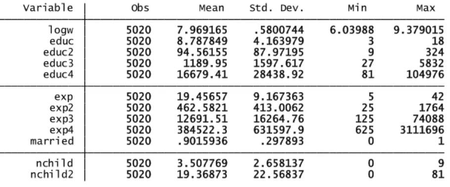
Appendix I – Data Summary

Table 1 – Data summary for Non-Jews in 1972

Table 2 – Data summary for Jews in 1972

nchild2 2561 21.5287 24.35963 0 81 nchild 2561 3.686451 2.818135 0 9 married 2561 .8969153 .3041289 0 1 exp4 2561 219624.7 396346.3 625 3111696 exp3 2561 8162.609 11335.05 125 74088 exp2 2561 338.49 324.1763 25 1764 exp 2561 16.4877 8.165281 5 42 educ4 2561 26299.37 21797.37 81 104976 educ3 2561 1963.641 1154.337 27 5832 educ2 2561 151.1597 58.74911 9 324 educ 2561 12.02421 2.56528 3 18 logw 2561 8.158991 .5838595 5.687825 9.05825 Variable Obs Mean Std. Dev. Min Max

. summarize logw educ educ2 educ3 educ4 exp exp2 exp3 exp4 married nchild nchild2 if year==1972 & nonjew==1

(20)

20 Table 4 – Data summary for Jews in 1983

Table 6 – Data summary for Jews in 1995

nchild2 8690 11.41979 14.7694 0 81 nchild 8690 2.63015 2.121939 0 9 married 8690 .8926352 .3095943 0 1 exp4 8690 288413.4 499207 625 3111696 exp3 8690 10177.95 13460.49 125 74088 exp2 8690 399.4429 358.9897 25 1764 exp 8690 18.15524 8.356935 5 42 educ4 8690 25588.49 31274.26 81 104976 educ3 8690 1787.534 1690.583 27 5832 educ2 8690 133.3886 88.29984 9 324 educ 8690 10.87031 3.902141 3 18 logw 8634 8.07942 .5658377 6.977226 9.924168 Variable Obs Mean Std. Dev. Min Max

(21)

21

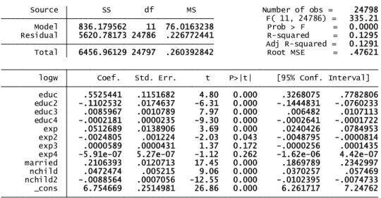
Appendix II – Regression Results

Table 7 – Regression Results for Non-Jews in 1972

Table 8 – Regression Results for Jews in 1972

_cons 7.257512 .5131751 14.14 0.000 6.25123 8.263795 nchild2 -.00241 .0016375 -1.47 0.141 -.0056209 .0008009 nchild .0357691 .0151295 2.36 0.018 .0061016 .0654366 married .1862564 .0452516 4.12 0.000 .0975226 .2749901 exp4 3.28e-06 1.65e-06 1.99 0.047 4.90e-08 6.51e-06 exp3 -.0002627 .0001425 -1.84 0.065 -.0005422 .0000167 exp2 .0064648 .004292 1.51 0.132 -.0019513 .0148809 exp -.0477294 .0525472 -0.91 0.364 -.150769 .0553102 educ4 -.0001208 .0000551 -2.19 0.029 -.0002288 -.0000127 educ3 .0047143 .0023841 1.98 0.048 .0000393 .0093892 educ2 -.0568657 .0361124 -1.57 0.115 -.1276783 .0139468 educ .2654689 .2237034 1.19 0.235 -.17319 .7041277 logw Coef. Std. Err. t P>|t| [95% Conf. Interval] Total 872.683453 2560 .340891974 Root MSE = .55567 Adj R-squared = 0.0942 Residual 787.059606 2549 .308771913 R-squared = 0.0981 Model 85.6238474 11 7.78398613 Prob > F = 0.0000 F( 11, 2549) = 25.21 Source SS df MS Number of obs = 2561

. regress logw educ educ2 educ3 educ4 exp exp2 exp3 exp4 married nchild nchild2 if year==1972 & nonjew==1

_cons 6.754669 .2514981 26.86 0.000 6.261717 7.24762 nchild2 -.0088564 .0007056 -12.55 0.000 -.0102395 -.0074733 nchild .0472474 .005215 9.06 0.000 .0370257 .057469 married .2106393 .0120713 17.45 0.000 .1869789 .2342997 exp4 -5.91e-07 5.27e-07 -1.12 0.262 -1.62e-06 4.42e-07 exp3 .0000589 .0000431 1.37 0.172 -.0000256 .0001435 exp2 -.0024805 .001224 -2.03 0.043 -.0048795 -.0000814 exp .0512689 .0138906 3.69 0.000 .0240426 .0784953 educ4 -.0002181 .0000235 -9.30 0.000 -.0002641 -.0001722 educ3 .0085967 .0010789 7.97 0.000 .006482 .0107113 educ2 -.1102532 .0174637 -6.31 0.000 -.1444831 -.0760233 educ .5525441 .1151682 4.80 0.000 .3268075 .7782806 logw Coef. Std. Err. t P>|t| [95% Conf. Interval] Total 6456.96129 24797 .260392842 Root MSE = .47621 Adj R-squared = 0.1291 Residual 5620.78173 24786 .226772441 R-squared = 0.1295 Model 836.179562 11 76.0163238 Prob > F = 0.0000 F( 11, 24786) = 335.21 Source SS df MS Number of obs = 24798

(22)

22 Table 9 – Regression Results for Non-Jews in 1983

_cons 6.372682 .2504935 25.44 0.000 5.881605 6.863759 nchild2 -.0042643 .0012119 -3.52 0.000 -.0066402 -.0018884 nchild .0339955 .0111752 3.04 0.002 .0120872 .0559038 married .0569363 .0320528 1.78 0.076 -.0059013 .1197738 exp4 -1.36e-06 8.54e-07 -1.59 0.111 -3.04e-06 3.12e-07 exp3 .0001421 .0000786 1.81 0.071 -.0000119 .0002961 exp2 -.0057137 .0025037 -2.28 0.023 -.010622 -.0008054 exp .1075961 .0323744 3.32 0.001 .0441281 .1710641 educ4 -.0001655 .0000332 -4.98 0.000 -.0002306 -.0001003 educ3 .0061903 .0013386 4.62 0.000 .003566 .0088145 educ2 -.0736766 .0183646 -4.01 0.000 -.1096792 -.037674 educ .3572128 .1012529 3.53 0.000 .1587129 .5557128 logw Coef. Std. Err. t P>|t| [95% Conf. Interval] Total 1688.82463 5019 .336486279 Root MSE = .54536 Adj R-squared = 0.1161 Residual 1489.45287 5008 .29741471 R-squared = 0.1181 Model 199.371767 11 18.1247061 Prob > F = 0.0000 F( 11, 5008) = 60.94 Source SS df MS Number of obs = 5020

_cons 6.043448 .1471657 41.07 0.000 5.754998 6.331899 nchild2 -.0153296 .0010586 -14.48 0.000 -.0174045 -.0132548 nchild .0882634 .006518 13.54 0.000 .0754879 .1010388 married .198267 .0126263 15.70 0.000 .1735189 .223015 exp4 -2.53e-06 4.14e-07 -6.12 0.000 -3.35e-06 -1.72e-06 exp3 .0002698 .0000365 7.39 0.000 .0001983 .0003413 exp2 -.0104349 .0011133 -9.37 0.000 -.012617 -.0082527 exp .1787158 .0137088 13.04 0.000 .151846 .2055856 educ4 -.0001337 .0000143 -9.35 0.000 -.0001618 -.0001057 educ3 .0050454 .0006184 8.16 0.000 .0038332 .0062575 educ2 -.061735 .0094668 -6.52 0.000 -.0802903 -.0431796 educ .3410046 .061247 5.57 0.000 .220958 .4610511 logw Coef. Std. Err. t P>|t| [95% Conf. Interval] Total 13120.7203 31812 .412445627 Root MSE = .57422 Adj R-squared = 0.2005 Residual 10485.829 31801 .329732683 R-squared = 0.2008 Model 2634.89125 11 239.535568 Prob > F = 0.0000 F( 11, 31801) = 726.45 Source SS df MS Number of obs = 31813

(23)

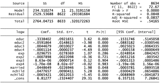
23 Table 11 – Regression Results for Non-Jews in 1995

_cons 6.81277 .2324407 29.31 0.000 6.357131 7.26841 nchild2 -.0065421 .0012013 -5.45 0.000 -.0088969 -.0041873 nchild .0477657 .0090411 5.28 0.000 .0300429 .0654886 married .0448649 .0226946 1.98 0.048 .0003781 .0893518 exp4 -1.70e-08 8.02e-07 -0.02 0.983 -1.59e-06 1.56e-06 exp3 8.63e-06 .0000714 0.12 0.904 -.0001313 .0001486 exp2 -.0007898 .0022098 -0.36 0.721 -.0051216 .003542 exp .0296755 .0278369 1.07 0.286 -.0248914 .0842425 educ4 -.0001114 .0000237 -4.69 0.000 -.000158 -.0000649 educ3 .0044679 .0010027 4.46 0.000 .0025023 .0064335 educ2 -.0591864 .0148613 -3.98 0.000 -.0883182 -.0300546 educ .3338402 .0921651 3.62 0.000 .1531746 .5145058 logw Coef. Std. Err. t P>|t| [95% Conf. Interval] Total 2764.04715 8633 .320172263 Root MSE = .54165 Adj R-squared = 0.0837 Residual 2529.53688 8622 .293381684 R-squared = 0.0848 Model 234.510274 11 21.3191158 Prob > F = 0.0000 F( 11, 8622) = 72.67 Source SS df MS Number of obs = 8634

_cons 6.039205 .2294659 26.32 0.000 5.589447 6.488963 nchild2 -.0246413 .0011767 -20.94 0.000 -.0269476 -.0223349 nchild .170381 .0064143 26.56 0.000 .1578089 .1829532 married .0452137 .0105709 4.28 0.000 .0244946 .0659329 exp4 -3.13e-06 4.82e-07 -6.50 0.000 -4.08e-06 -2.19e-06 exp3 .0003015 .000041 7.35 0.000 .0002211 .000382 exp2 -.0102629 .0012162 -8.44 0.000 -.0126466 -.0078792 exp .1563533 .0146113 10.70 0.000 .1277149 .1849917 educ4 -.0001325 .0000176 -7.53 0.000 -.000167 -.000098 educ3 .0051585 .0008058 6.40 0.000 .0035791 .0067379 educ2 -.0660491 .0132003 -5.00 0.000 -.0919219 -.0401762 educ .3870421 .0914623 4.23 0.000 .2077741 .5663102 logw Coef. Std. Err. t P>|t| [95% Conf. Interval] Total 17959.2856 41051 .437487165 Root MSE = .59623 Adj R-squared = 0.1874 Residual 14589.1099 41040 .355485134 R-squared = 0.1877 Model 3370.1757 11 306.379609 Prob > F = 0.0000 F( 11, 41040) = 861.86 Source SS df MS Number of obs = 41052

(24)

24

Appendix III – Comparative Data Table

Table 13

1972 1983 1995

Jews Non-Jews Jews Non-Jews Jews Non-Jews

Coefficient Mean Coefficient Mean Coefficient Mean Coefficient Mean Coefficient Mean Coefficient Mean Constante 6.75467 7.25751 6.04345 6.37268 6.03921 6.81277 educ 0.55254 13.841 0.26547 12.024 0.34100 11.998 0.35721 8.788 0.38704 13.132 0.33384 10.870 educ2 -0.11025 197.41 -0.05687 151.16 -0.06174 160.384 -0.07368 94.562 -0.06605 183.333 -0.05919 133.39 educ3 0.00860 2893.9 0.00471 1963.6 0.00505 2312.2 0.00619 1190.0 0.00516 2687.0 0.00447 1787.5 educ4 -0.00022 43565 -0.00012 26299 -0.00013 35217 -0.00017 16679 -0.00013 41017 -0.00011 25588 exp 0.05127 18.275 -0.04773 16.488 0.17872 19.171 0.10760 19.457 0.15635 19.823 0.02968 18.155 exp2 -0.00248 420.01 0.00646 338.49 -0.01043 453.46 -0.00571 462.58 -0.01026 465.65 -0.00079 399.44 exp3 0.00006 10941 -0.00026 8162.6 0.00027 12355 0.00014 12692 0.00030 12163 0.00001 10178 exp4 0.00000 305877 0.00000 219625 0.00000 368996 0.00000 384522 0.00000 340621 0.00000 288413 married 0.21064 0.9023 0.18626 0.8969 0.19827 0.8818 0.05694 0.9016 0.04521 0.8473 0.04486 0.8926 nchild 0.04725 2.0636 0.03577 3.6865 0.08826 1.9791 0.03400 3.5078 0.17038 1.8156 0.04777 2.6302 nchild2 -0.00886 7.1747 -0.00241 21.529 -0.01533 6.0333 -0.00426 19.369 -0.02464 5.2423 -0.00654 11.420 N 24798 2561 31813 5020 41052 8634 R2 0.12950 0.09810 0.20080 0.11810 0.18770 0.08480

Wage Discrimination Between Jews and Non-Jews in Israel

Rapport de recherche