HAL Id: hal-02990899
https://hal.archives-ouvertes.fr/hal-02990899
Submitted on 5 Nov 2020
HAL is a multi-disciplinary open access archive for the deposit and dissemination of sci-entific research documents, whether they are pub-lished or not. The documents may come from teaching and research institutions in France or abroad, or from public or private research centers.
L’archive ouverte pluridisciplinaire HAL, est destinée au dépôt et à la diffusion de documents scientifiques de niveau recherche, publiés ou non, émanant des établissements d’enseignement et de recherche français ou étrangers, des laboratoires publics ou privés.
A control approach to scheduling flexibly configurable
jobs with dynamic structural-logical constraints
Dmitry Ivanov, Boris Sokolov, Weiwei Chen, Semyon Potryasaev, Alexandre
Dolgui, Frank Werner
To cite this version:
Dmitry Ivanov, Boris Sokolov, Weiwei Chen, Semyon Potryasaev, Alexandre Dolgui, et al.. A con-trol approach to scheduling flexibly configurable jobs with dynamic structural-logical constraints. IISE Transactions, Taylor & Francis, 2021, 53 (1), pp.21-38. �10.1080/24725854.2020.1739787�. �hal-02990899�
Preprint
D. Ivanov, B. Sokolov, W. Chen, A. Dolgui, S. Potryasaev, F. Werner. A control approach to scheduling flexibly con-figurable jobs with dynamic structural-logical constraints, IISE Transactions, 2021, vol. 53, n° 1, p. 21–38,
doi.org/10.1080/24725854.2020.1739787
A control approach to scheduling flexibly configurable jobs with dynamic
structural-logical constraints
Abstract
This study theorizes how the optimal control paradigm can be applied to modeling and algorithmic solutions in manufacturing systems with dynamically changing hybrid structural-logical-terminal con-straints. Our study conceptualizes and operationalizes a unique class of problems with both flexible machines and flexible jobs that can be frequently encountered in manufacturing systems with individu-alized products when process and schedule are created simultaneously. We offer a model to schedule jobs in manufacturing systems when the structural-logical terminal constraints are changing dynami-cally, and an algorithm to obtain a tractable solution analytically within the proven axiomatic of the optimal program control and mathematical optimization. We develop a dynamic decomposition meth-odology for modeling and control of schedules in highly flexible production systems combining the advantages of continuous and discrete optimization. The findings suggest that our approach can be of value for approaching problems with a simultaneous process design (i.e., task composition) and opera-tion sequencing (i.e., service composiopera-tion). Utilizing the outcomes of this research could also support the consideration of dynamics in the operations control. The operations execution can be accurately modeled in continuous time as state variables the updates of which allow for data-driven control of machine availability and capacity disturbances. Besides, the method developed theorizes further gener-alized insights into decomposition methods for scheduling and is supported by an analytical analysis and an algorithmic realization.
1. Introduction
Modelling and control in manufacturing have been frequently considered in light of flexible or recon-figurable systems, where multiple flexible machines are divided into modules to perform different tasks (Li and Meerkov 2009, Dolgui and Proth 2010). The machine flexibility allows for dynamically chang-ing process technologies (i.e., flexibly arischang-ing jobs through customer-specific sequencchang-ing of operations) to achieve the product individualization and variety (Balakrishnan and Geunes 2003, Koren et al. 2016). However, the issues of scheduling of flexibly arising jobs have not been explicitly treated in the domain of reconfigurable systems. In scheduling, most of the problems presume a fixed processing technology for product manufacturing (Pinedo 2018). At the same time, the recent literature provides a number of insights on the scheduling with flexible jobs, especially in relation to digital manufacturing (Ivanov et al. 2016, Ahn et al. 2018, Liu et al. 2018).
Our study aims at integrating the two above-mentioned domains – flexible machines and flexible jobs – within a unified methodological framework. The recent literature (Dolgui et al. 2019) points to a special class of modeling and control problems with hybrid structural-logical-terminal constraints which are frequently encountered in customized manufacturing systems with individualized products when the process design and job sequencing are performed simultaneously (Battaia et al. 2018, Kusiak et al. 2018). The structural constraints usually relate to the process design while logical (i.e., precedence) constraints are concerned with job sequencing, and the terminal constraints are encountered in both process design and scheduling. One difficulty in modelling such problems is that those constraints are changing dynamically in time due to availabilities of machines and individual job structuring by opera-tions.
Examples of such systems stem from new digital manufacturing paradigms such as Industry 4.0 and cloud manufacturing which bring new challenges to the scheduling community. In digital manufactur-ing, the process planning and job scheduling are integrated due to the usage of services instead of the rigid and fixed allocations of operations and machines (Frazzon et al. 2018, Rossit et al. 2018). These new technologies are enabling a highly flexible production, particularly through the use of
cyber-phys-ical systems and customized assemblies in order to deliver manufacturing services on-demand to con-sumers (Nayak et al. 2016, Ahn et al. 2018, Battaïa et al. 2018, Frazzon et al. 2018, Tao et al. 2018, Yang et al. 2019).
We build on and contribute to the literature on manufacturing systems with flexible machines and flex-ible jobs. The studies on reconfigurable manufacturing systems (Youssef and ElMaraghy 2006, Borto-lini et al. 2018) and multi-stage, flexible, job-flow shop scheduling problems with flexible machines (Kyparisis and Koulamas 2006, Ivanov et al. 2016a,b, Bozek and Werner 2017) are the closest research streams to this new emerging scheduling area in the era of Industry 4.0. Another relevant research field for our study is the resource-constrained project scheduling with alternative activity chains (Tao and Dong 2017, Blazewicz et al. 2019). While providing the profound results for problems with a combina-tion of either structural-terminal constraints (Kreter et al. 2016), or structural-logical constraints (Tao and Dong 2017), or structural-logical constraints (Battaïa et al. 2017), none of these research fields, however, comprehensively treats the combination of both flexible machines, and flexible jobs, as well as flexible dynamic structural-logical-terminal constraints – a substantive and distinctive contribution made by our study.
Many problems known in those and other relevant domains are already NP-complete as decision prob-lems, and pose challenges to the mathematical programming and optimization communities even for fixed processes (Kyparis and Koulamas 2006, Tahar et al. 2006, Jungwattanakit et al. 2009, Tran and Ng 2011, Vallada et al. 2017). If the process fixation would now be released as posited in Industry 4.0 and cloud manufacturing, those problems would become even harder to formulate and to solve both in decision and in computational spaces. The traditional paradigm of tackling such a problem is to solve a mathematical program in the planning stage, and resolve the problem with updated information in sched-uling. However, under the flexible manufacturing setup, the frequency of an information update is typ-ically too fast to respond by solving mathematical programming models. The process flexibility may also render the solution obtained in the planning stage meaningless. As such, modeling and solution methods for the simultaneous structural-functional synthesis of the process design and scheduling in systems with decentralized computational activities and dynamically changing resource availabilities need to be further developed using a different paradigm.
Our study brings the discussion further and explores the domain of scheduling with dynamically chang-ing structural-terminal-logical constraints by framchang-ing the decision-makchang-ing problem and the decomposi-tion technique in terms of optimal control blended with discrete optimizadecomposi-tion. We believe that the control theory can propose interesting frameworks to design scheduling problems when utilizing its combina-tions with local search or other traditional combinatorial optimization approaches. This is to say that the control paradigms can be useful to design frameworks in manufacturing scheduling in an integration with discrete optimization scheduling techniques.
There are several argumentations to support the necessity to explore new optimization techniques for scheduling in customized manufacturing systems looking at the interface of control and discrete optimi-zation. First, scheduling in digital manufacturing exhibits a specific characteristic, i.e., a simultaneous synthesis of the processing technology (planning) and scheduling. As such, scheduling is now consid-ered as a combination of process (task) composition and service composition which happen simultane-ously, so the process and schedule are created at the same time. The known solutions in discrete optimi-zation based on mathematical decomposition or relaxation have tackled some of these problems (e.g., Kaskavelis and Caramanis, 1998), but others remain challenging. More recent decomposition ideas, such as data-driven or clustering approaches (Chen et al. 2013a,b), are founded on the difficulties in deriving analytical properties. Metaheuristics or heuristics have also been widely used in solving these problems, such as job shop scheduling (Barnes and Chambers 1995; Lobo et. al. 2014), but no solution-quality guarantee can be provided. Second, a peculiarity of scheduling in digital manufacturing is its data-driven nature that, at the same time, becomes favorable for the development of new dynamic ap-proaches to modelling those problems based on decomposition methods (Ivanov et al. 2016a, Rossit et al. 2018, Xu et al. 2019). We are not aware of any published formulation of those problems using math-ematical programs which consider the dynamically changing structural-terminal-logical constraints. Even if such a new problem could be formulated as a mathematical program by finding an innovative form to describe the dynamically changing constraints/flexibilities as equations/inequalities, it is diffi-cult to imagine an efficient solution technique as for now. The main peculiarity is that both the manu-facturing process structures and the resource/machine availabilities are changing in time.
In summary, our study makes the following contributions to the literature. First and principally, we offer a model to describe the manufacturing scheduling problem with dynamically changing structural-termi-nal-logical constraints and an algorithm to obtain a tractable solution analytically within the proven axiomatic of the optimal control and mathematical optimization. We build on and contribute to the lit-erature on scheduling in highly flexible and digital manufacturing, decomposition principles in flexible shop scheduling, and scheduling by optimal control. We consider a unique combination of both flexible machines, and flexible jobs, and flexible dynamic structural-logical-terminal constraints. With all that, our study conceptualizes and operationalizes a unique class of manufacturing control problems when the process and schedule are created simultaneously and the hybrid structural-terminal-logical con-straints are subject to dynamic changes in time.
The remainder of this paper is as follows. Sect. 2 conducts a survey on the related literature and sum-marizes the main contributions of this paper. In Sect. 3, the problem under study is introduced, and the optimal control model is presented. Sect. 4 develops the computational procedure for solving the model, and illustrate the algorithm using an example. Finally, Sect. 5 concludes the paper by summarizing the most important results of this study and outlining some issues for future research.
2. State of the Art
The theoretical foundations of our approach build on four theoretical perspectives, namely reconfigura-ble manufacturing systems, flexireconfigura-ble job scheduling, scheduling in digital manufacturing, and resource-constrained project scheduling. While the first and the latter ones can be considered as conceptual ena-blers of our study, the second and third perspectives have a closer relationship to the technical imple-mentation. As such, and in light of the limited length of the paper, we restrict ourselves to their analysis. A growing body of research has reported advances in dealing with flexible flow shop scheduling. Ky-paris and Koulamas (2006) considered a multi-stage, flexible flow shop scheduling problem with uni-form parallel machines at each stage and makespan minimization. This study proposed a heuristic algo-rithm for this strongly NP-hard problem. Tazar et al. (2006) considered a scheduling problem for a set of independent jobs with sequence-dependent setup times and job splitting on a set of identical parallel machines such that the maximum completion time (i.e., the makespan) is minimized. For this NP-hard problem, the study developed a heuristic algorithm using linear programming (LP). Furthering these
insights, Bożek and Werner (2018) developed an optimization method for flexible job shop scheduling with lot streaming and sublot size optimization. The recent literature has included a variety of principles and approaches to the design and scheduling of flexible and reconfigurable assembly systems with a focus on balancing, scheduling, and sequencing (Delorme et al. 2012, Battaïa et al. 2017). In these stud-ies, models and methods have been presented for solving problems related to the optimization of the performance intensity of an assembly system for sets of flexibly intersecting operations. In particular, in scheduling with alternative parallel machines at each stage of the manufacturing process, alternative machines may execute the operations. Some research reported associations between the flexibility in the process plan and an increased complexity in both the machine assignment and sequencing of tasks (Yu et al. 2011, Blazewicz et al. 2015, Chen et al. 2018). An extensive body of the literature has been devel-oped on simultaneously selected process plans and schedules as well as on scheduling with changing availability of resources, predominantly rooted in discrete optimization techniques. One can refer to the frameworks of multi-processor flow shops, hybrid flow tshops with identical machines, unrelated par-allel machine problems with machine and job selection, distributed assembly permutation flow shops, multi-objective hybrid flow shop problems, and complex hybrid flexible flowline problems (Jung-wattanakit et al. 2009, Tran and Ng 2011, Fanjul and Ruiz 2012, Vallada et al. 2017).
The second perspective directs the attention to the main specifics of scheduling in digital manufacturing. The paper by Ivanov et al. (2016a) was among the first studies conducted on the impact of Industry 4.0 on manufacturing scheduling. It proposed a model and algorithm based on a combination of continuous and discrete optimization that allows for representing schedules in the form of optimal control trajecto-ries which are dynamically driven by data transformed to state and control variables. Frazzon et al. (2018) underlined the role of digitalization to apply data-driven adaptive planning and control. The data integration between the real manufacturing system and the simulation model was implemented through a data-driven framework. Ivanov et al. (2018) considered proactive scheduling and reactive real time control in Industry 4.0 manufacturing systems and developed a concept and model of data-driven sched-ule optimization. Rossit et al. (2018) developed a concept of smart scheduling, aiming to yield flexible and efficient production schedules that are formed dynamically, in an event-oriented matter. In smart manufacturing, the processes for different customer orders may have individual structures of the stations
such that the flexible stations are able to execute different functions subject to individual sets of opera-tions within the jobs (Ivanov et al. 2016a,b, Nayak et al. 2016, Battaïa et al. 2017, Zhong et al. 2017). Such a perspective on the integrated problem of simultaneous, structural-functional synthesis of the Industry 4.0 customized assembly systems and job scheduling appears to be more relevant in a practical decision environment, relative to inherent problems in incorporating changes in the environment and production system itself.
Similar approaches have been developed in the area of cloud manufacturing, the concept of which aims to deliver manufacturing services to consumers on-demand. Liu et al. (2018) pointed out task composi-tion and service composicomposi-tion as two dominants in scheduling in cloud manufacturing. Task composicomposi-tion is a prerequisite for scheduling of tasks in cloud manufacturing. Service composition is a combination of multiple services, atomic or composite, into value-added services to fulfil a task or a set of tasks. Ahn et al. (2018) analyzed the selection of services from the cloud manufacturing platform and combining them to a process by task composition.
The analysis of the concept of services leads to two fundamental specifics of digital manufacturing. The first one is the production system redundancy, and the second one is the computational redundancy. The production system redundancy is driven by industrial Internet-of-Things (IoT) which transforms pro-duction processes from rigid links between operations and machines to a variety of flexible allocations. The computational redundancy arises due to the furnishing of the machines and products with compu-tational and data processing devices, allowing performing some computations directly by machines and products and using Cloud and Fog computational technologies. These two redundancies create a princi-pally new entity for manufacturing modelling and control, i.e., a service. The services can realize almost any combination of machines and operations (Ivanov et al. 2016a, Ahn et al. 2018, Liu et al. 2018). None of these studies, though, formally and rigorously modelled the manufacturing systems with mixed structural-terminal-logical constraints and considering the data-driven schedule updates – a distinctive and significant contribution made by our study.
In summary, the studies on scheduling in Industry 4.0, smart manufacturing, and cloud manufacturing differ regarding the methodologies but most of them share a certain set of the following attributes: (a)
simultaneous structural-functional synthesis of the customized assembly system, (b) data-driven sched-uling based on the communication of the products and stations with a resulting reduction of the combi-natorial complexity, and (c) resemblance to flexible multi-processor flow shop scheduling. For example, in the manufacturing platform MindSphere which is a cloud-based, open IoT operating system, products, plants, systems, and machines are connected to enable the usage of data generated by the IoT with ad-vanced analytics in schedule optimization (Siemens 2018). Usage of autonomous mobile robots (AMR) makes it possible to implement almost any flexibility in the manufacturing processes even with the traditional assembly line stations (Nielsen et al. 2017). However, in previous studies, the selection of the process structure and the respective station functionality for the execution of the operations were considered in isolation. In many cloud manufacturing, such an integration can have a significant impact on the process efficiency (Liu et al. 2018). The problem of a simultaneous structural-functional synthesis of the customized assembly system is still at the beginning of its investigation. Previously isolated in-sights gained in hybrid shop scheduling and sequencing with alternative parallel machines, resource constrained project scheduling with alternative chains, reconfigurable manufacturing system design and optimal control scheduling models with both terminal and logical constraints can now be integrated into a unified framework of Industry 4.0 and require an extension towards models with hybrid structural-terminal-logical constraints (Dolgui et al. 2019). With that being said, doubts have been raised as to whether efficient solutions can be proposed to the scheduling problems with combined logical-structural constraints using traditional discrete optimization paradigms which directs our attention to continuous optimization and control theory.
While the automatic control community has developed a body of knowledge for scheduling of manu-facturing, sensor systems and real-time scheduling of dynamic control systems (Burgess and Passino 1999, Sethi et al. 2000, Aicardi et al. 2008, Park and Yang 2009, Mati and Xie 2011, Vincent and Pon-nambalam 2013, Han et al. 2017), the use of a control paradigm for manufacturing scheduling is still restricted despite of a proven resemblance of the manufacturing systems to control systems (Feng and Yan 2000, Ivanov et al. 2018, Dolgui et al. 2019, Sokolov et al. 2018). As a result, it is not yet clear how the control paradigm can be applied to scheduling in highly flexible systems of the digital manufactur-ing.
Our method combines the advantages of continuous and discrete optimization. Specifically, our study develops an optimal control model and algorithm for the simultaneous structural-functional design of a customized manufacturing process and the sequencing of the operations within the jobs. The developed theoretical framework presents a contribution to flexible scheduling in the emerging field of Industry 4.0-based innovative production systems. We mention that this study extends previous publications of the authors (Ivanov et al. 2016a,b), where only scheduling decisions were considered and the design of the process structure was assumed to be fixed, i.e., the design of a flow shop process was considered. In this paper, the scheduling model considers the structural synthesis and sequencing decisions of the man-ufacturing process, and therefore it forms a more complicated problem structure, where the scheduling control framework becomes critical in solving large-scale dynamic problems.
A distinctive feature of our approach is that we propose to decompose dynamically the large-scale as-signment matrix according to the precedence relations between the operations of the jobs and dynami-cally consider only the operations that satisfy these precedence relations at a given time point in small-dimensional, discrete optimization models. Discrete optimization algorithms are used for scheduling in these matrices of small dimension at each time point. Continuous optimization algorithms (e.g., the method of successive approximations, or the method of Krylov-Chernousko, see Ivanov et al. 2016 and Dolgui et al. 2019, and the references in these papers) are used to create a schedule from the discrete optimization results generated at each time point by extremizing the Hamiltonian function at each time point subject to some criteria (e.g., tardiness). The present study applies the dynamic decomposition method to fully flexible flow shops with both alternative input and output precedence relations (cf. Fig. 3 later in the paper). Such a combination is unique in the literature, as it mimics the complexity of modern manufacturing reality affording more realistic applications.
The findings suggest that our approach can be of value for problems with a simultaneous process design (i.e., task composition) and operation sequencing (i.e., service composition). Utilizing the outcomes of this research can also help to accurately model the dynamics of the operations execution in continuous time as state variables the updates of which allow for a data-driven control of machine availability and capacity disturbances. The distinctive and significant contribution made by our study is that the
con-structed modelling paradigm (scheduling control framework, combining discrete optimization and opti-mal control) is explicitly capable of capturing dynamic features in digital manufacturing, which are difficult to model using the traditional mathematical programming paradigm. Such scenarios are chal-lenging to model as a linear relationship in discrete optimization, but are convenient to describe using the continuous control paradigm to address the complexity of the dynamically changing hybrid struc-tural-logical-terminal constraints by decomposition principles. We should point out that the proposed approach does not replace the mathematical modeling approaches. Instead, it supplements the existing approaches in tackling a set of problems with new requirements (i.e., dynamically changing hybrid structural-logical-terminal constraints) emerging in digital manufacturing.
3. Scheduling Control Modelling Methodology
In this section, we present the scheduling control modeling methodology. 3.1 Problem Description
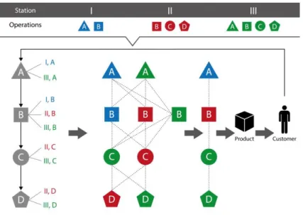
We now introduce the problem to be solved. Specifically, consider a customer job control system which interacts with an assembly system while the latter offers services to solve particular tasks in the job control system ((Fig. 1).
Fig. 1. Interaction of the customer and the assembly systems
The customer system generates orders (jobs) each of which has an individual sequence of the techno-logical operations resulting in individual task composition. Each of these sequences requires an individ-ual service composition. The interaction of the customer and the assembly systems results in alternatives
for the design of the manufacturing process. Each station has multiple channels, each of which is dedi-cated to a set of technological operations. Multiple stations may perform equal operations and alterna-tives for job scheduling and sequencing exist resulting in dynamic logical constraints which are, in turn subject to actual capacity utilization, machine availability, and time- and cost-related parameters of the services which represent terminal constraints. As such, there are dynamic structural constraints on the process design.
In Fig. 1, a customer order (i.e., a job) is considered which contains the four operations A, B, C, and D. Three flexible workstations are considered. Station I is capable of processing operations A and B, station II is capable of processing operations B, C, and D, and station III is capable of processing all operations A, B, C, and D. The first task is to design the manufacturing process, i.e., to perform a task composition by combining technological operations into a manufacturing process. In other words, the sequencing of operations into a process is performed. The second task is to implement a service composition by as-signing the operations to stations at each stage of the technological process.
Such a problem shows a set of special features. For example, the dynamically changing operations se-quences in the tasks may impose dynamic and nonlinear requirements in the constraints for the machine and operations control. Machine maintenance requirements and schedules can depend on its assigned tasks and sequence of operations, and thus the machine availability and capacity may change dynami-cally as a result, sometimes in a nonlinear relationship with time. Such dynamic and nonlinear con-straints could be hard to model and capture in the traditional mathematical programming paradigm. In the next section, we propose a scheduling model for the given problem class with hybrid structural-functional-logical constrains which is based on a dynamic interpretation of the operations execution processes.
3.2 Model
Let us introduce the following basic sets and structures (the indices (O), (П) and (Р) describe the rela-tions of the sets to the operarela-tions, flows, and resources, respectively).
𝐴 = {𝐴𝑖, 𝑖 = 1, … , 𝑛} is the set of customer orders (jobs).
𝑀 = {𝑀𝑗, 𝑗 = 1, … , 𝑚} is the set of resources (e.g., stations or machines; these terms are used as
𝐷(𝑖)= {𝐷𝜅(𝑖), 𝜅 = 1, … , 𝑆𝑖} is the set of operations which can be executed in the system.
𝑃 = {𝑃𝜅(𝑖), 𝜅 = 1, … , 𝑆𝑖} is the set of material, energy or information flows in the process.
An intersection of the sets M, D, and P is a service; i.e., an entity needed to fulfill a process step in the set A. The services are formed dynamically based on the available machines and operations.
Assume that the manufacturing and transportation capacities may be disrupted and
- the station availability is described by a given preset matrix time function 𝜀𝑖𝑗(𝑡) of time-spatial
con-straints: we have 𝜀𝑖𝑗(𝑡) = 1, if the station is available and 𝜀𝑖𝑗(𝑡) = 0, otherwise;
- the station ability to process operations can be described by the set 𝛩 whose element 𝛩𝑖𝜅𝑗 is equal to
1 if station 𝑀𝑗 has the ability to process an operation 𝐷𝜅(𝑖), and equals 0, otherwise;
- the capacity dynamics can be described by a continuous function of the perturbation impacts 𝜉𝑗(𝑡);
𝜉𝑗(𝑡) = 1 if 100% available, 𝜉𝑗(𝑡) = 0 if the capacity is fully disrupted, and 𝜉𝑗(𝑡) = [0;1] in the case
of partial unavailability.
The formal statement of the scheduling problem is based on a dynamic interpretation of the execution processes of the services. Let us introduce some new notations.
Parameters
𝑎𝑖𝜅(Ο), 𝑎𝑖𝜅(Π) are the normative and actual flow times of each operation. The values of these parameters are related to the end conditions to be reached in 𝑥𝑖𝜅(Ο),𝑥𝑖𝜅(Π) at 𝑡 = 𝑡𝑓. While the normative time 𝑎𝑖𝜅(Ο) is
fixed and known in advance, the actual operation execution time 𝑎𝑖𝜅(Π)is computed during the optimiza-tion procedure by varying the processing intensities at the machines subject to the objective funcoptimiza-tion extremization.
𝑐𝑖𝜅𝑗(Π) is the maximum processing intensity for the operation 𝐷𝜅(𝑖) at the 𝑀𝑗; it determines the maximum
possible value for the production quantity for the operation 𝐷𝜅(𝑖) described by the control variable 𝑢𝑖𝜅𝑗(Π). 𝜇𝑗 is the manufacturing costs per time unit at 𝑀𝑗
Decision variables
𝑥𝑖𝜅(Π) is a state variable characterizing the actual flow time of the operation 𝐷𝜅(𝑖) at each moment 𝑡; 𝑥𝑖𝜅(Π) can be varied (i.e., expedited and slowed down) according to variation of 𝑐𝑖𝜅𝑗(Π)
𝑥𝑗(Ρ) is a state variable characterizing the run time of the station 𝑀𝑗;
𝑢𝑖𝜅𝑗(Ο)(𝑡), 𝜔𝑖𝜅𝑗(Ο)(𝑡) are control variables.
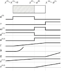
The meaning of the auxiliary (marked with index B) variables
𝑣, 𝜔(Ο), 𝑢(𝐵,1), 𝑢(𝐵,2), 𝑧, ℎ, 𝑔, 𝑥(𝐵,1), 𝑥(𝐵,2) is explained below and shown in Fig. 2.
Fig. 2. Auxiliary control variable dynamics
z
is an auxiliary variable which characterizes the execution of the k-operation,h
is the square under the integral curvez
, andg
is an auxiliary variable which is equal to the time point t between the completion time of the k-operation and tf . The meaning of the other auxiliary variables will beex-plained in the context of the constraint system (7)-(20). These auxiliary variables are used to fulfill the non-preemption condition for operations. The modeling procedure for the non-preemption of operations is shown in (Ivanov et al. 2013 and Sokolov et al. 2018).
Let us illustrate the general logical-dynamic mathematical model of the manufacturing process design and control. The problem statement described above implies both the process design and operation se-quencing. As such, scheduling problems with hybrid structural-terminal-logical constraints must be analyzed (Dolgui et al. 2019). Consider the simplified example of a system with hybrid
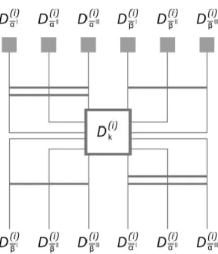
Fig. 3. Precedence relations of operation 𝐷𝜅(𝑖) In Fig. 3, the operation 𝐷𝜅(𝑖) follows the operations 𝐷𝛼̄/
(𝑖)
𝐷𝛼̄//
(𝑖)
𝐷𝛼̄///
(𝑖)
according to the “AND” precedence rule (meaning that all the operations𝐷𝛼̄/
(𝑖)
𝐷𝛼̄//
(𝑖)
𝐷𝛼̄///
(𝑖)
should be completed to start 𝐷𝜅 (𝑖)
; those operations are noted by index α) and the operations 𝐷𝛽̄/
(𝑖)
𝐷𝛽̄//
(𝑖)
𝐷𝛽̄///
(𝑖)
according to the precedence rule “OR” (meaning that at least one of the operations 𝐷𝛽̄/
(𝑖)
𝐷𝛽̄//
(𝑖)
𝐷𝛽̄///
(𝑖)
should be completed to start 𝐷𝜅 (𝑖)
; those operations are noted by index β). Analogously, the six operations follow the operation 𝐷𝜅
(𝑖)
according to either “and” or “or” rules. The combination of “AND” and “OR” precedence and follower relations results in dy-namic logical constraints which represent the highly flexible set of available technological process de-signs (task composition) and service compositions.
For the system considered, the optimal control model can be written as Eqs. (1)-(3).
𝑥̇𝑖𝜅(Ο)= ∑ 𝜀𝑖𝜅𝑗(𝑡) ⋅ 𝛩𝑖𝜅𝑗(𝑢𝑖𝜅𝑗 (Ο)(𝑡) + 𝜔 𝑖𝜅𝑗 (Ο)(𝑡)) 𝑚 𝑗=1 , ∀𝑖, 𝜅 (1) 𝑥̇𝑖𝜅(Π)= ∑ 𝑢𝑖𝜅𝑗(Π)(𝑡) 𝑚 𝑗=1 , ∀𝑖, 𝜅 (2) 𝑥̇𝑗(Ρ)= ∑ ∑ 𝑢𝑖𝜅𝑗(Ο)(𝑡) 𝑆𝑖 𝜅=1 𝑛 𝑖=1 , ∀𝑗 (3)
Eq. (1) describes the dynamics of the operation execution for the job 𝐴𝑖. If 𝑥̇𝑖𝜅
(Ο)= ∑ 𝑢
𝑖𝜅𝑗
(Ο)(𝑡)
𝑚
𝑗=1 , then at
pro-cessing is in progress at the 𝑀𝑗. Eq. (1) can be interpreted as a resource project scheduling model
de-scribing the network of operations. Eq. (2) describes the actual execution of the operations. Subject to the different possible operation assignments to the stations, 𝑥̇𝑖𝜅(Π) can be expedited by accelerating the machine or selecting the fastest machine or slowed down. This processing progress is reflected by an increase in 𝑢𝑖𝜅𝑗(Π)(𝑡), e.g., with each additional output unit produced. Eq. (3) describes the dynamics of the station utilization. In case of 𝑢𝑖𝜅𝑗(Ο)(𝑡) = 0, the station does not produce anything at time t. Similarly, if 𝑢𝑖𝜅𝑗(Π)(𝑡) = 0, the product is not processed at time t.
Eqs. (1)-(3) are interconnected. While the process design (i.e., the technology synthesis) is described by Eq. (1), the sequencing is controlled by Eq. (2) by adjusting the flow time through the selection of processing intensities which allows to extremize the objective function. At the same time, the results of the process design directly affect the machine utilization using Eq. (3). In other words, Eqs. (1)-(3) describe the dynamic structural-functional synthesis of a flexible manufacturing system.
Eqs. (4)-(6) describe the requirements on the non-preemption of the operations and the numerical as-sessment of the number of completed operations as well as on the determination of the operation com-pletion time, respectively.
𝑧̇𝑖𝜅𝑗 = 𝑢𝑖𝜅𝑗(Ο)+ 𝜔𝑖𝜅𝑗(Ο); ℎ̇𝑖𝜅𝑗= 𝑧𝑖𝜅𝑗; 𝑔̇𝑖𝜅𝑗 = 𝑣𝑖𝜅𝑗, ∀𝑖, 𝜅, 𝑗 (4)
𝑥̇𝑖𝜅(𝐵,1)= 𝑢𝑖𝜅(𝐵,1), ∀𝑖, 𝜅 (5)
𝑥̇𝑖𝜅(𝐵,2)= 𝑢𝑖𝜅(𝐵,2), ∀𝑖, 𝜅 (6)
The constraint system can be described as shown in Eqs. (7)-(20).
∑ 𝑢𝑖𝜅𝑗(П)(𝑡) 𝑚 𝑗=1 ≤ 1 , ∀ 𝑖, 𝜅; ∑ ∑ 𝑢𝑖𝜅𝑗(Ο)(𝑡) 𝑆𝑖 𝜅=1 𝑛 𝑖=1 ≤ 1, ∀𝑗 (7) ∑ 𝑢𝑖𝛼̄𝑗(Ο) 𝑚 𝑗=1 ⋅ ∑ 𝑥𝑖𝜅(Ο) 𝜅∈𝛤𝑖𝛼̄+ = 0, ∀𝑖, 𝛼̄ (8) ∑ 𝑢𝑖𝛽̄𝑗(Ο) 𝑚 𝑗=1 ⋅ ∏ 𝑥𝑖𝜅(Ο) 𝜅∈𝛤 𝑖𝛽̄ + = 0, ∀𝑖, 𝛽̄ (9)
∑ 𝑢𝑖𝛼̄̄𝑗(Ο) 𝑚 𝑗=1 ⋅ ∑ (𝑎𝑖𝜅(Π)− 𝑥𝑖𝜅(Π)) 𝜅∈𝛤𝑖𝛼̄̄− = 0, ∀𝑖, 𝛼̄̄ (10) ∑ 𝑢 𝑖𝛽̄̄𝑗 (Ο) 𝑚 𝑗=1 ⋅ ∏ (𝑎𝑖𝜅(Π)− 𝑥𝑖𝜅(Π)) 𝜅∈𝛤 𝑖𝛽̄̄ − = 0, ∀𝑖, 𝛽̄̄ (11) ∑ 𝜔𝑖𝜅𝑗(Ο)[𝑎𝑖𝜅(Π)− 𝑥𝑖𝜅(Π)] 𝑚 𝑗=1 = 0, ∀𝑖, 𝜅 (12) 𝜔𝑖𝜅𝑗(Ο)⋅ 𝑔𝑖𝜅𝑗 = 0, ∀𝑖, 𝜅, 𝑗 (13) 𝑣𝑖𝜅𝑗[𝑎𝑖𝜅 (Ο) − ∑ 𝑧𝑖𝜅𝑗 𝑚 𝑗=1 ] = 0, ∀𝑖, 𝜅, 𝑗 (14) i s n ( П ) (f ) (f ) ikj j i 1 k 1 u (t) R (t)
, ∀𝑖, 𝜅, j (15) 𝑢𝑖𝜅(𝐵,1)⋅ 𝑥𝑖𝜅(𝐵,2)= 0, ∀𝑖, 𝜅 (16) 𝑢𝑖𝜅(𝐵,2)[𝑎𝑖𝜅(Π)− 𝑥𝑖𝜅(Π)] = 0, ∀𝑖, 𝜅 (17) 0 ≤ 𝜉𝑗(𝑡) ≤ 1, ∀𝑗 (18) 0 ≤ 𝑢𝑖𝜅𝑗(Π)≤ 𝑐𝑖𝜅𝑗(Π)𝑢𝑖𝜅𝑗(Ο)(𝑡)𝜉𝑗(𝑡), ∀𝑖, 𝜅, 𝑗 (19) 𝑢𝑖𝜅𝑗(Ο)(𝑡), 𝜔𝑖𝜅𝑗(Ο)(𝑡), 𝑢𝑖𝜅(𝐵,1)(𝑡), 𝑢𝑖𝜅(𝐵,2)(𝑡) ∈ {0,1}, ∀𝑖, 𝜅, 𝑗 (20) The structural constraints (7) determine the number of operations that can be simultaneously processed at a station. By default, this number is 1. The logical constraints are represented by Eqs. (8)-(12). Eqs. (8) and (9) define precedence relations for operation 𝐷𝜅(𝑖)
with regard to the predecessor operations 𝐷𝛼̄(𝑖), 𝐷𝛽̄(𝑖). Constraints (10) and (11) define precedence relations for operation 𝐷𝜅(𝑖) with regard to the subse-quent operations 𝐷𝛼̄̄(𝑖), 𝐷
𝛽̄̄ (𝑖)
. Constraint (12) defines the logic for the auxiliary control variable 𝜔𝑖𝜅𝑗(Ο)∈ {0,1} which equals 1 if 𝑥𝑖𝜅(Π)(𝑡) = 𝑎𝑖𝜅(Π) at time point 𝑡 and 𝑥𝑖𝜅(Ο)≠ 𝑎𝑖𝜅(Ο). In other words, the flow pro-cessing is completed. To compensate this, an auxiliary control 𝜔𝑖𝜅𝑗(Ο) is introduced in Eq. (12). Constraints (13) and (14) are used to avoid overproduction regarding the operation 𝐷𝜅(𝑖), i.e., 𝑥𝑖𝜅(Ο)(𝑡𝑓) = 𝑎𝑖𝜅
(Ο)
, which means that 𝑥𝑖𝜅(Ο)(𝑡𝑓) cannot exceed 𝑎𝑖𝜅
(Ο)
(f ) j
R of the station 𝑀𝑗. Eq. (15) is used jointly with constraints (13) and (14) to avoid interruptions of an
operation execution (Ivanov et al. 2013). With the help of constraints (16) and (17), the jobs can be counted at 𝑡 = 𝑡𝑓 for which all the required operations 𝐷𝜅
(𝑖)
are completed. In order to assess the schedule robustness (e.g., using attainable sets), we introduce a constraint on perturbation (18). Eq. (19) is a ter-minal capacity constraint on the operation processing subject to the maximum processing intensity 𝑐𝑖𝜅𝑗(Π) at the stations. Since 𝑐𝑖𝜅𝑗(Π) is different at various stations, the flow time of an operation is also variable depending on the station selection. With the help of Eq. (19), the state variables 𝑥𝑖𝜅(Ο) and 𝑥𝑖𝜅(П) are con-nected. If 𝑢𝑖𝜅𝑗(Ο)(𝑡) = 1, then we have a run of job 𝐷𝜅(𝑖) using 𝑀𝑗, and 𝑢𝑖𝜅𝑗
(Ο)(𝑡) = 0 otherwise; 𝜔 𝑖𝜅𝑗 (Ο)(𝑡) =
1 at the moment when 𝑥𝑖𝜅(Π)= 𝑎𝑖𝜅(Π) , and 𝜔𝑖𝜅𝑗(Ο)(𝑡) = 0 at the moment when 𝑥𝑖𝜅(Ο)= 𝑎𝑖𝜅(Ο). Constraints (19) are used jointly with constraints (15). The latter determines the speed of the operations execution at the station while (19) determines the upper capacity limits at each station for all the operations exe-cuted at this station. Eq. (20) is a binary constraint.
Eqs. (8)-(12) can be considered as active dynamic constraints meaning that the number of operations in those constraints is changing dynamically in time in relation to Eqs. (1)-(3). The expressions in Eqs. (8)-(12) are to equal zero if, and only if control variables are equal to 1 which means that all the predecessor operations have been executed. This leads by tendency to the constraint system of a small dimensionality at each point of time that can be resolved using discrete optimization techniques for integer and linear programming. Along with the operations, flow and station dynamics in process control models (1)-(3), the dynamic changes in constraints (8)-(12) determine the dimensionality of the scheduling problem in a discrete optimization model at each point of time that consists of the constraints (17)-(20) subject to the criteria (23)-(24) and (26)-(28). Note that constraints (17)-(20) correspond to a canonical form of mathematical programming scheduling models.
The boundary conditions can be written as shown in Eqs. (21) and (22). 𝑡 = 𝑡0: 𝑥𝑖𝜅 (Ο) (𝑡𝑜) = 𝑥𝑖𝜅 (Π) (𝑡𝑜) = 𝑥𝑗 (Ρ) (𝑡𝑜) = 𝑧𝑖𝜅𝑗(𝑡𝑜) = 𝑢𝑖𝜅𝑗(𝑡𝑜) = 𝑔𝑖𝜅𝑗(𝑡𝑜) = 0 𝑥𝑖𝜅(𝐵,1)(𝑡𝑜) = 0; 𝑥𝑖𝜅 (𝐵,2) (𝑡𝑜) = 0; (21) 𝑡 = 𝑡𝑓: 𝑥𝑖𝜅 (Ο) (𝑇𝑓) = 𝑎𝑖𝜅 (Ο) ; 𝑥𝑖𝜅(𝑓)(𝑡𝑓) = 𝑎𝑖𝜅 (𝑓) (22)
𝑥𝑖(Π)(𝑡𝑓), 𝑧𝑖𝜅𝑗(𝑡𝑓), ℎ𝑖𝜅𝑗(𝑡𝑓), 𝑔𝑖𝜅𝑗(𝑡𝑓), 𝑥𝑖𝜅 (𝐵,1)
(𝑡𝑓), 𝑥𝑖𝜅 (𝐵,2)
(𝑡𝑓) ∈ ℜ1, ℜ1∈ [0, . . . , ∞)
The control functions are introduced in Eqs. (23)-(28). 𝐽1= 1 2∑ ∑ (𝑎𝑖𝜅 (Ο) − 𝑥𝑖𝜅(Ο))2 𝑆𝑖 𝜅=1 𝑛 𝑖=1 → 𝑚𝑖𝑛 (23) 𝐽2 = 1 2∑ ∑ (𝑎𝑖𝜅 (Π)− 𝑥 𝑖𝜅 (Π))2 𝑆𝑖 𝜅=1 𝑛 𝑖=1 → 𝑚𝑖𝑛 (24) 𝐽3= 1 2∑ ∑ [(𝑎𝑖𝜅 (Ο)− ∑ 𝑧 𝑖𝜅𝑗 𝑚 𝑗=1 )2+ ∑(𝑧𝑖𝜅𝑗𝑔𝑖𝜅𝑗+ (𝑎𝑖𝜅)2 2 − ℎ𝑖𝜅𝑗) 2𝑧 𝑖𝜅𝑗2 𝑚 𝑗=1 ] 𝑡=𝑡𝑓 → 𝑚𝑖𝑛 𝑠𝑖 𝜅=1 𝑛 𝑖=1 (25) 𝐽4= ∑ (𝑥𝑗 (Ρ)(𝑡 𝑓) ∙ 𝜇𝑗) 2 𝑚 𝑗=1 → 𝑚𝑖𝑛 (26) 𝐽5= 1 2∑ (𝑥𝑖𝜅 (𝐵,1) (𝑡𝑓)) 2 𝑠𝑖 𝜅=1 → 𝑚𝑖𝑛 (27) 𝐽6= (𝐽1 (𝑚𝑖𝑛) − 𝐽1(𝜉))(𝐽2(𝑚𝑖𝑛)− 𝐽2(𝜉)) → 𝑚𝑖𝑛 (28)
Eqs. (23) and (24) are used to estimate the fullness of operation fulfillment subject to the planned vol-umes aik. Eq. (25) considers a non-preemptive execution of an operation. Eq. (26) reflects the costs
incurred at 𝑡 = 𝑡𝑓, where 𝜇𝑗 is the manufacturing cost per time unit at the 𝑀𝑗. Eq. (27) is used to estimate
the fullfillment of operation 𝑖 in time. The lower the value of J5 , the shorter the makespan. Eq. (28) is
used to estimate the schedule robustness using attainable sets (Ivanov and Sokolov 2010, Ivanov et al. 2016a,b) which enables a feasibility analysis of a two-point boundary problem.
4. Solution Algorithm
In this section, we present the solution algorithm that solves the model proposed in Section 3. Most centrally, we would like to point out that this study does not intend to enter a computational competition with the other known solution techniques for the studied problem but rather conceptualizes an entirely new viewpoint. This study theorizes how optimal control paradigms can be used to design a framework for modeling and optimal algorithmic solutions for scheduling problems with dynamically changing hybrid structural-logical-terminal constrains; one practical example of such problems is an integrated task and service composition in digital manufacturing scheduling.
The modelling and computational procedures are methodologically unified within the axiomatic of op-timal control theory and based on using continuous state variables to determine the start and completion
times of the manufacturing service realization. The discrete control variables are used to compose ser-vices by assigning operations to the machines at different steps in the process. The execution of opera-tions is described with the help of continuous state variables. The control variables of the operaopera-tions are binary and discrete aiming at the assignment of operations to machines to form a service. The flow control variables are continuous and describe the actual volume of executed operations. The flow and operations control are interconnected through the logical-dynamic constraints (10)-(12).
4.1. Computational Principles
The major algorithmic idea proposed in this research is to decompose the assignment matrix dynami-cally in time, considering polynomially solvable (by tendency) problems of small dimensionality at each time point (see Fig. 4 for an example). In the example illustrated in Fig. 4, six jobs are considered, each of which contains a sequence of operations that can be executed at four alternative workstations. At time point t=t1, the operations D62, D51, D41, D31, D21, and D12 are available for an assignment to machines
subject to the precedence relations. Therefore, a small-dimensional assignment problem with six opera-tions and four machines arises at time point t=t1 which is solved using standard discrete optimization
techniques. As a result, the operations D62, D51, D31, and D12 are assigned to the machines M(4), M(3),
M(2), M(1), respectively. This is indicated by the control variables u
624, u513, u312, and u121, which are
switched to 1. Similarly, at time point t=t2, we deal with a small-dimensional assignment problem with
six operations and four machines. As a result, the operations D63, D41, D22, and D13 are assigned to the
Fig. 4. Dynamic decomposition principle
To summarize and generalize the example in Fig. 4, the small dimensionality at each time point results from the dynamic decomposition described by the constraints on the precedence relations, i.e., at each time point we consider only those operations that can be assigned to machines at that time point, ex-cluding those operations that have already been completed and those that cannot start because the pre-decessors are not completed yet. By dynamically decomposing the assignment matrix in time, we rep-resent the optimal control problem as a two-point boundary problem, then to treat polynomially solvable problems (by tendency) of small dimensionality at each time point, and finally to integrate the partial solutions through the maximum principle by integrating the main and adjoint equation systems.
It is commonly known that analytical methods for an optimal control have been proven for small-di-mensional systems. In the control engineering practice, numerical methods have been applied. Recent surveys of those methods have been presented by Dolgui et al. (2019) and Sokolov et al. (2018). A methodical challenge in applying the maximum principle is to find the coefficients of the adjoint system which change in dynamics. Another methodical challenge of boundary problems is that the initial con-ditions for the adjoint variables (T0) are not given. At the same time, an optimal control should be
calculated subject to the end conditions.
According to Dolgui et al. (2019), numerical methods can be classified into state space (i.e., direct meth-ods, e.g., gradient methods), control space (i.e., indirect methods based on control variations such as the method of successive approximations), and trajectory space (e.g., dynamic programming method) meth-ods. The system space method is based on the optimal control problem presentation as a two-point boundary problem using the maximum principle and is rooted in deriving necessary conditions of opti-mal control. Two systems of differential equations are solved: the main system and the conjugate one. This provides an optimal program control vector u*(t) and the state trajectory x*(t). The vector u*(t)
at time tT0 under the conditions h0
x(T0)
O and for the given value of ψ(T0) returns the maximumto the Hamiltonian function. The missing initial conditions of the adjoint system are computed based on different algorithms, e.g., considering a constructive heuristic solution.
Considering the constraints (4)-(20), we suggest a combination of system and control space methods while integrating optimal control and mathematical programming. Optimal control is not used for solv-ing the combinatorial problem, but rather for enhancsolv-ing the existsolv-ing mathematical programmsolv-ing algo-rithms regarding non-stationarity, flow control, and continuous material flows. Since the control varia-bles are presented as binary variavaria-bles, methods of discrete optimization are applied to combinatorial tasks within certain time intervals. The proposed specialized computational method is valid for special control system classes such as linear systems, where methods and algorithms for quadratic linear prob-lems are applied, or when the optimal control problem is presented as discrete optimization.
4.2. Computational Procedure
The following algorithm has been developed and tested to compute an optimal solution. We refer to the study (Ivanov et al. 2016a) for an optimality and complexity analysis of the computational procedure that has been used in this study as an anchor. The computational procedure for the developed model (Eqs. (1)-(3)) is based on the integration of the main and adjoint equation systems subject to the maxi-mization of the Hamiltonian (29)-(35):
𝛨(𝒙(𝑡), 𝒖(𝑡), 𝝍(𝑡)) = 𝛨1+ 𝛨2+ 𝛨3+ 𝛨4+ 𝛨5+ 𝛨6+ 𝛨7, where 𝛨1= ∑ ∑ ∑[𝜓𝑖𝜅 (Ο) 𝜀𝑖𝜅𝑗(𝑡)𝛩𝑖𝜅𝑗+ 𝜓𝑗 (Ρ) + 𝜑𝑖𝜅𝑗(1)] ⋅ 𝑢𝑖𝜅𝑗(Ο) 𝜇 𝑗 𝑖 (29) 𝛨2= ∑ ∑ ∑[𝜓𝑖𝜅 (Π) ] ⋅ 𝑢𝑖𝜅𝑗(Π) 𝑗 𝜇 𝑖 (30) 𝛨3= ∑ ∑ ∑[𝜑𝑖κ𝑗 (1) + 𝜓𝑖κ(Ο)∙ 𝜀𝑖𝜅𝑗∙ 𝛩𝑖κ𝑗] ⋅ 𝜔𝑖κ𝑗 (Ο) 𝑗 κ 𝑖 (31) 𝛨4= ∑ ∑ ∑ 𝜑𝑖κ𝑗 (2) ⋅ 𝑧𝑖κ𝑗 𝑗 κ 𝑖 (32) 𝛨5= ∑ ∑ ∑ 𝜑𝑖κ𝑗 (3) ⋅ 𝜈𝑖κ𝑗 𝑗 κ 𝑖 (33) 𝛨6= ∑ ∑ 𝑝𝑖κ (𝐵,1) ⋅ 𝑢𝑖κ(𝐵,1) κ 𝑖 (34) 𝛨7= ∑ ∑ 𝑝𝑖κ (𝐵,2) ⋅ 𝑢𝑖κ(𝐵,2) 𝜇 𝑖 (35)
The algorithm is formally introduced as follows.
Algorithm 1: DYN-CONTROL
0. Set 𝑡 = 0, and initialize all parameters.
1. From the time point 𝑡 = 𝑡0 onwards, determine the control 𝒖(𝑟+1)(𝑡) (𝑟 = 0,1,2, . .. denotes the number of the
iteration).
2. For the given initial boundary conditions (21) and 𝝍(𝑡0), compute 𝒖∗(𝑡) at t=t0 to maximize (29)-(35).
a) Solve the assignment problem: solve the maximization of the Hamiltonian 𝐻1 for model (1), (3) with
constraints (7), (20).
b) Solve the linear programming problem: solve the maximization of the Hamiltonian 𝐻2 for model (2) with
constraints (15), (18), (19).
c) Operation selection: select operations and constraints which meet the requirements (7), (18), (19), (20).
3. 𝒖∗(𝑡
0) is then put into (1)-(6) and (36)-(53)
4. Main and adjoint systems are integrated.
5. The transversality conditions (54)-(61) are evaluated
6. Update 𝑡 → 𝑡1.
7. 𝒖∗(𝑡
1) is computed based on Hamiltonian (29)-(35) maximization, where t1 = t0+ (is the chosen integration
step). 𝒙(𝑟)(𝑡
1) is generated.
8. If 𝑡 = 𝑡𝑓, then the record value 𝐽𝐺= 𝐽𝐺
(𝑟)
can be calculated.
9. The integration process is continued as long as the end boundary conditions (22) are reached and the
conver-gence for 𝐽𝐺 is realized.
10. The resulted 𝒖(∗)(𝑡) is the optimized schedule.
Consider the algorithmic realization in more detail. The continuous optimization part can be described as follows. In order to compute the optimal program control vector 𝒖∗(𝑡) and the corresponding state trajectory 𝒙∗(𝑡), the main (1)-(6) and adjoint (36)-(52) systems need to be solved. In accordance with the maximum principle, the adjoint system = ‖𝜓𝑖𝜅(Ο)𝜓𝑖𝜅(Π)𝜓𝑗(Ρ)𝜑𝑖𝜅𝑗(1)𝜑𝑖𝜅𝑗(2)𝜑𝑖𝜅𝑗(3)𝑝𝑖𝜅(𝐵,1)𝑝𝑖𝜅(𝐵,2)‖𝑇 can be written corresponding to the main system (1)-(6) 𝒙 = ‖𝑥𝑖𝜅(Ο)𝑥𝑖𝜅(Π)𝑥𝑗(Ρ)𝑧𝑖𝜅𝑗ℎ𝑖𝜅𝑗𝑔𝑖𝜅𝑗𝑥𝑖𝜅
(𝐵,1)
𝑥𝑖𝜅(𝐵,2)‖𝑇 (see Appendix
2). The transversality conditions can be formulated in the way shown in Appendix 3. The analytical form of the computation of the coefficients is presented in Ivanov et al. (2016a).
For the given initial boundary conditions (21) and 𝝍(𝑡0), the 𝒖∗(𝑡) at t=t0 is computed to maximize
(29)-(35). 𝒖∗(𝑡
The optimal program control vector at time 𝑡 = 𝑡0 for the given value of 𝝍(𝑡) returns the maximum to
(29)-(35), which can be transformed into a general performance index and expressed in scalar form 𝐽𝐺.
Next, 𝒖∗(𝑡1) is computed based on Hamiltonian (29)-(35) maximization, where
t
1=
t0+ (is thecho-sen integration step). As a result of the dynamic model run at each iteration, 𝒙(𝑟)(𝑡) is generated. The adjoint system (36)-(53) (see Appendix 2) is integrated subject to 𝒖(𝑡) = 𝒖̄(𝑡) and over the interval from 𝑡 = 𝑡𝑓 to 𝑡 = 𝑡0. In addition, if 𝑡 = 𝑡𝑓, then the record value 𝐽𝐺 = 𝐽𝐺
(𝑟)
can be calculated. After this, the transversality conditions (54)-(61) are evaluated (see Appendix 3). The dynamic coordination pa-rameters are the adjoint variables which change their values during the iterative process of the solution of the corresponding two-point boundary problem. The integration process is continued as long as the end boundary conditions (22) are reached and the convergence for 𝐽𝐺 is reached.
Now let us turn to the discrete optimization part. Since the stations are flexible and can process multiple operations, the assignment problem exists. The maximization of the Hamiltonian 𝐻1 (Eq. 29) for model
(1), (3) in combination with the constraints (7), (20) solves the assignment problem. The maximum number of operations that can be assigned to a station is determined in Eq. (7). Due to the dynamic decomposition principle state above, the assignment matrix at each time point is smaller.
The maximization of the Hamiltonian 𝐻2 (Eq. 30) for model (2) in combination with the constraints (15)
(18), (19) solves the linear programming problem. At each time point, only operations and constraints which meet the requirements (7), (18), (19), (20) are considered. By a dynamic switching of constraints (8)-(17), the size of the scheduling problem at each time point is reduced. The Hamiltonians (30) and (31) can be maximized when the constraints (13) and (19) satisfy the corresponding variables 𝜔𝑖𝜅𝑗(Ο) and 𝑢𝑖κ𝑗(Π). In this case, only a part of the constraints (8)-(17) is considered for the current assignment problem since, when the control in (8)-(17) is switched to 1, it becomes active in the right-hand part of the equa-tions (1), (2), (3). Therefore, the reduction of the problem dimensionality at each time point in the cal-culation process is ensured because of the recurrent operation description. At each time point, the Ham-iltonian function is extremized. The locally coordinated sub-problems are partial combinatorial assign-ment problems and linear programming problems which are formed dynamically depending on the prec-edence relations, the channel availability at the stations, and the operation execution progress.
In the algorithm, the search for an optimal control in each iteration is performed in the class of boundary (e.g., pointwise or relay) functions which correspond to the discrete nature of decision making in sched-uling. The formulated model is a linear, non-stationary, finite–dimensional controlled system of differ-ential equations with a convex area of feasible control. This model form satisfies the conditions of the existence theorem in Lee and Markus (1967, Theorem 4, Corollary 2), which allows us to assert the existence of an optimal solution in the appropriate class of feasible controls. The algorithm optimality and sufficiency proofs can be found in the study (Ivanov et al. 2016a).
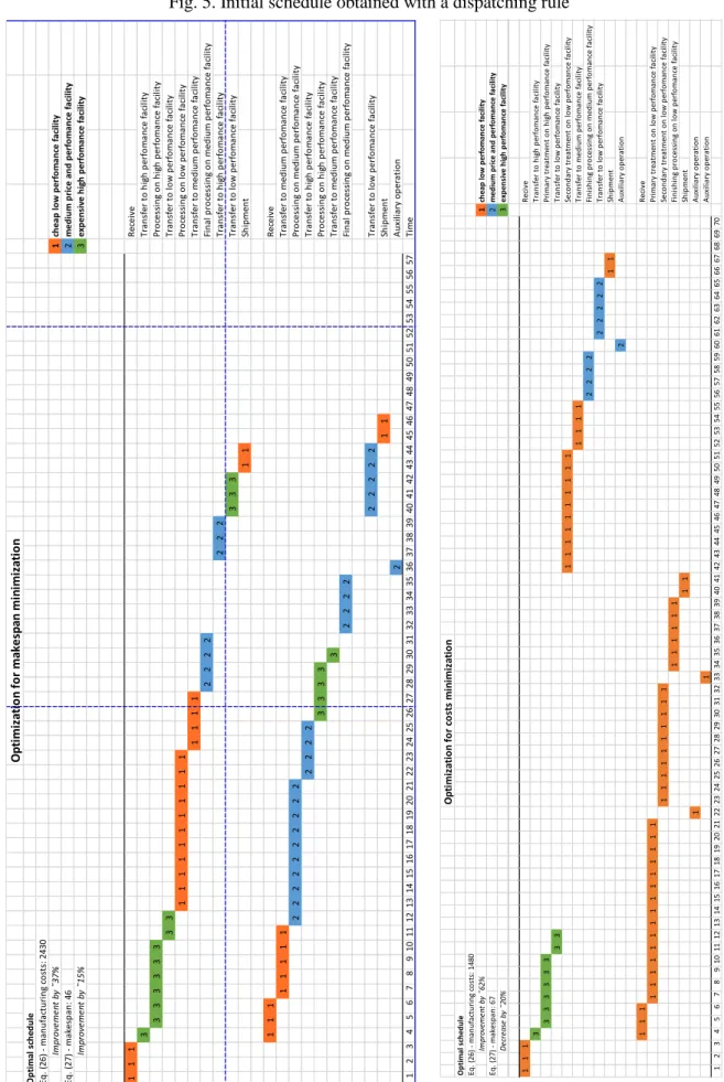
4.3. Illustrative Example
Consider an example with two jobs, three stations of different performance (slow and cheap, medium, fast and expensive), and three operations of each job. The processing of the operations at the station differs regarding the costs and time which results in a trade-off of manufacturing costs (Eq. 26) and makespan (Eq. 27). In Figs 5 and 6, a real-life example of a digital manufacturing system in the ship yard industry modelled using the developed control approach is depicted as a Gantt chart for two jobs. Nodes 1 and 5 are the source and sink nodes of the control trajectories. Nodes 7, 8, and 9 correspond to the operation execution at the medium performance station 2 (M2). Nodes 2, 3, and 4 correspond to the
operation execution at the slow and cheap station 1 (M1). Nodes 21, 22, and 23 correspond to operation
execution at the fast and expensive station 3 (M3).
The algorithmic procedure is launched by an arbitrary feasible schedule 𝒖̃ (𝑡), 𝑡 ∈ (𝑇0, 𝑇𝑓] according to
the initial conditions (21) (Fig. 5). Fig. 6 displays the optimal control trajectories obtained for the exam-ple from Fig. 5 for an optimization against costs and makespan. Two jobs take a different control de-pending on the preferences in the objective function in terms of costs vs makespan minimization. In the case of makespan minimization (Fig. 6a), we have manufacturing costs (Eq. 26) of $2430 in the optimal schedule which represents an improvement in comparison with the initial schedule generated by a dis-patching rule at Step 1 of the algorithm by about 37%. The makespan (Eq. 27) is 46 time units, i.e., it is improved by about 15% as compared to the initial schedule generated. In the case of cost minimization (Fig. 6b), the manufacturing costs (Eq. 26) of $1480 can be observed resulting in an improvement in comparison with the initial schedule by about 62%. The makespan is 67 time units implying a longer
time-to-customer by about 20% as compared to the initial schedule generated. The cheap and slow sta-tion M1 is mostly used in the case of cost minimization whereas a mix of different stations can be
ob-served in the schedule computed for the makespan minimization.
O p ti mi za ti o n f o r ma ke sp an mi n imi za ti o n Sc h ed u le b y d isp atc h in g ru le 1 ch ea p lo w p er fo m an ce f ac ili ty Eq . ( 26 ) - ma n u fa ct u ri n g co st s: 3 86 0 2 m ed iu m p ri ce a n d p er fo m an ce f ac ili ty Eq . ( 27 ) - ma kes p an : 5 4 3 ex p en si ve h ig h p er fo m an ce f ac ili ty 1 1 1 R ec ei ve 1 1 Tra n sf er to h ig h p erf o ma n ce fa ci lit y 3 3 3 3 3 3 Pro ces si n g o n h ig h p erf o ma n ce fa ci lit y 3 3 3 3 Tra n sf er to med iu m p erf o ma n ce fa ci lit y 2 2 2 2 2 2 2 Pro ces si n g o n med iu m p erf o ma n ce fa ci lit y 2 2 Tra n sf er to h ig h p erf o ma n ce fa ci lit y 3 3 Fi n al p ro ces si n g o n h ig h p erf o ma n ce fa ci lit y 3 3 3 Tra n sf er to med iu m p erf o ma n ce fa ci lit y 2 2 2 2 2 Tra n sf er to lo w p erf o ma n ce fa ci lit y 1 1 Sh ip men t 1 1 1 R ec ei ve 3 Tra n sf er to h ig h p erf o ma n ce fa ci lit y 3 3 3 3 3 3 Pro ces si n g o n h ig h p erf o ma n ce fa ci lit y 3 3 3 Tra n sf er to med iu m p erf o ma n ce fa ci lit y 2 2 2 2 2 2 2 Pro ces si n g o n med iu m p erf o ma n ce fa ci lit y 2 2 2 Tra n sf er to h ig h p erf o ma n ce fa ci lit y 3 3 Fi n al p ro ces si n g o n h ig h p erf o ma n ce fa ci lit y 3 3 3 Tra n sf er to med iu m p erf o ma n ce fa ci lit y 2 2 2 2 2 Tra n sf er to lo w p erf o ma n ce fa ci lit y 1 1 Sh ip men t 1 2 3 4 5 6 7 8 9 10 11 12 13 14 15 16 17 18 19 20 21 22 23 24 25 26 27 28 29 30 31 32 33 34 35 36 37 38 39 40 41 42 43 44 45 46 47 48 49 50 51 52 53 54 55 56 57 Ti me
Fig. 5. Initial schedule obtained with a dispatching rule O p ti mi za ti o n f o r ma ke sp an mi n imi za ti o n O p ti m al sc h ed u le Eq . ( 26 ) - ma n u fa ct u ri n g co st s: 2 43 0 Im pr ov em en t by ˜3 7% 1 ch ea p lo w p er fo m an ce f ac ili ty Eq . ( 27 ) - ma kes p an : 4 6 2 m ed iu m p ri ce a n d p er fo m an ce f ac ili ty Im pr ov em en t by ˜1 5% 3 ex p en si ve h ig h p er fo m an ce f ac ili ty 1 1 1 R ec ei ve 3 Tra n sf er to h ig h p erf o ma n ce fa ci lit y 3 3 3 3 3 3 Pro ces si n g o n h ig h p erf o ma n ce fa ci lit y 3 3 Tra n sf er to lo w p erf o ma n ce fa ci lit y 1 1 1 1 1 1 1 1 1 1 1 Pro ces si n g o n lo w p erf o ma n ce fa ci lit y 1 1 1 1 Tra n sf er to med iu m p erf o ma n ce fa ci lit y 2 2 2 2 Fi n al p ro ces si n g o n med iu m p erf o ma n ce fa ci lit y 2 2 2 Tra n sf er to h ig h p erf o ma n ce fa ci lit y 3 3 3 Tra n sf er to lo w p erf o ma n ce fa ci lit y 1 1 Sh ip men t 1 1 1 R ec ei ve 1 1 1 1 1 Tra n sf er to med iu m p erf o ma n ce fa ci lit y 2 2 2 2 2 2 2 2 2 2 Pro ces si n g o n med iu m p erf o ma n ce fa ci lit y 2 2 2 2 Tra n sf er to h ig h p erf o ma n ce fa ci lit y 3 3 3 3 Pro ces si n g o n h ig h p erf o ma n ce fa ci lit y 3 Tra n sf er to med iu m p erf o ma n ce fa ci lit y 2 2 2 2 Fi n al p ro ces si n g o n med iu m p erf o ma n ce fa ci lit y 2 2 2 2 2 Tra n sf er to lo w p erf o ma n ce fa ci lit y 1 1 Sh ip men t 2 A u xi lia ry o p era ti o n 1 2 3 4 5 6 7 8 9 10 11 12 13 14 15 16 17 18 19 20 21 22 23 24 25 26 27 28 29 30 31 32 33 34 35 36 37 38 39 40 41 42 43 44 45 46 47 48 49 50 51 52 53 54 55 56 57 Ti me O p ti mi za ti o n f o r co st s mi n imi za ti o n O p ti m al sc h ed u le Eq . ( 26 ) - ma n u fa ct u ri n g co st s: 1 48 0 Im pr ov em en t by ˜6 2% 1 ch ea p lo w p er fo m an ce f ac ili ty Eq . ( 27 ) - ma kes p an : 6 7 2 m ed iu m p ri ce a n d p er fo m an ce f ac ili ty D ec re as e by ˜2 0% 3 ex p en si ve h ig h p er fo m an ce f ac ili ty 1 1 1 R ec ive 3 Tra n sf er to h ig h p erf o ma n ce fa ci lit y 3 3 3 3 3 3 Pri ma ry t rea tmen t o n h ig h p erf o ma n ce fa ci lit y 3 3 Tra n sf er to lo w p erf o ma n ce fa ci lit y 1 1 1 1 1 1 1 1 1 1 Sec o n d ary t rea tmen t o n lo w p erf o ma n ce fa ci lit y 1 1 1 1 Tra n sf er to med iu m p erf o ma n ce fa ci lit y 2 2 2 2 Fi n is h in g p ro ces si n g o n med iu m p erf o ma n ce fa ci lit y 2 2 2 2 2 Tra n sf er to lo w p erf o ma n ce fa ci lit y 1 1 Sh ip men t 2 A u xi lia ry o p era ti o n 1 1 1 R ec ive 1 1 1 1 1 1 1 1 1 1 1 1 1 1 1 Pri ma ry t rea tmen t o n lo w p erf o ma n ce fa ci lit y 1 1 1 1 1 1 1 1 1 1 Sec o n d ary t rea tmen t o n lo w p erf o ma n ce fa ci lit y 1 1 1 1 1 1 Fi n is h in g p ro ces si n g o n lo w p erf o ma n ce fa ci lit y 1 1 Sh ip men t 1 A u xi lia ry o p era ti o n 1 A u xi lia ry o p era ti o n 1 2 3 4 5 6 7 8 9 10 11 12 13 14 15 16 17 18 19 20 21 22 23 24 25 26 27 28 29 30 31 32 33 34 35 36 37 38 39 40 41 42 43 44 45 46 47 48 49 50 51 52 53 54 55 56 57 58 59 60 61 62 63 64 65 66 67 68 69 70
a) Makespan minimization b) Cost minimization Fig. 6. Optimal schedule obtained by control algorithm
5. Conclusions
The new technologies enable manufacturing with highly customized assembly systems and create a number of new remarkable challenges and opportunities for scheduling. In particular, the manufacturing processes for different customer orders may have individual machine structures such that the flexible stations are able to execute different functions subject to individual sets of operations within the jobs. Therefore, the problem of a simultaneous structural-functional synthesis of the systems with task and service compositions arises that in turn, feeds the challenging scheduling problems with dynamic hybrid structural-logical-terminal constraints. Our investigation accounts for this kind of scheduling problems with mixed structural-terminal-logical constraints when product and process are created at the same time. Examples of such systems have been increasingly encountered in digital manufacturing, e.g., in cloud manufacturing and Industry 4.0.
Our approach allows for revealing several insights which are difficult to receive with the help of other methods. First, the dynamic control model and dynamically changing constraints with the use of an original decomposition principle allow implicitly observing and controlling the variety of the process designs and schedule alternatives. Second, the constructed dynamic decomposition principle allows for dynamic control of constraints which appear and disappear in time from the dimensionality of the dis-crete optimization problems in the course of computational procedure due to precedence relations. Third, the proposed modelling paradigm makes it possible to consider the real-time information in the control framework as it becomes available with the help of updating the continuous state variables. In summary and in contrast to previous studies which assumed a fixed process design, our approach is capable of designing simultaneously the manufacturing process in regard to the available alternative stations, their current capacity utilization and the processing time, and the sequencing of the jobs. The use of state control variables in our model allows for updates in operations status that in turn, feeds automated in-formation feedbacks and control of schedule execution and disruption detection. The latter can be used
for launching the re-scheduling procedure, comprehensively combining the planning and adaptation de-cision within a unified methodological framework of dynamic control theory. In addition, a wide range of analysis tools from control theory regarding stability, controllability, adaptability, etc. may be used for the schedule analysis when described in terms of control.
In the future, a robustness analysis of the overall system, i.e., both of the process design and the schedule, can extend the results of this study. In addition, computational examples may help to reveal new insights. A more detailed analysis of the Industry 4.0 technology may illuminate a taxonomy of structural-func-tional problems in this emerging research field. Finally, Industry 4.0 and digital technologies open new possibilities to the implementation of dynamic scheduling techniques using real-time data about the machine utilization, entering of new jobs and the operation processing status. This makes it possible to extend the algorithmic dynamic decomposition principles of the control scheduling models, e.g., by incorporating an event-oriented decomposition based on such events as “a machine becomes available”, “an operation is completed” or “a new job enters the system”. These extensions can be considered in light of future research topics.
References
Ahn, G., Park Y.-J., & S. Hur (2018) Performance computation methods for composition of tasks with multiple patterns in cloud manufacturing, International Journal of Production Research, DOI: 10.1080/00207543.2018.1451664
Aicardi M., Giglio D., Minciardi R. (2008). Optimal strategies for multiclass job scheduling on a single machine with controllable processing times. IEEE Trans on Automatic Control 53(2), 479-495.
Balakrishnan, A., J Geunes (2003). Production planning with flexible product specifications: an appli-cation to specialty steel manufacturing. Operations Research 51 (1), 94-112.
Barnes, J.W., Chambers, J.B. (1995) Solving the job shop scheduling problem with tabu search. IIE Transactions, 27(2): 257-263.
Battaïa, O., A Otto, F Sgarbossa, E Pesch (2018). Future trends in management and operation of assem-bly systems: from customized assemassem-bly systems to cyber-physical systems. Omega 78, 1-4.
Battaïa, O., Dolgui, A., Guschinsky, N. (2017) Decision support for design of reconfigurable rotary machining systems for family part production. Int Journal of Production Research, 55(5), 1368-1385.