DIMENSIONAL ANALYSIS AND SURROGATE MODELS FOR THERMAL MODELLING OF POWER ELECTRONIC COMPONENTS

HAL Id: hal-02044714

https://hal.insa-toulouse.fr/hal-02044714

Submitted on 21 Feb 2019

HAL is a multi-disciplinary open access

archive for the deposit and dissemination of

sci-entific research documents, whether they are

pub-lished or not. The documents may come from

teaching and research institutions in France or

abroad, or from public or private research centers.

L’archive ouverte pluridisciplinaire HAL, est

destinée au dépôt et à la diffusion de documents

scientifiques de niveau recherche, publiés ou non,

émanant des établissements d’enseignement et de

recherche français ou étrangers, des laboratoires

publics ou privés.

ELECTRONIC COMPONENTS

F. Sanchez, Marc Budinger, Ion Hazyuk

To cite this version:

F. Sanchez, Marc Budinger, Ion Hazyuk. DIMENSIONAL ANALYSIS AND SURROGATE

MOD-ELS FOR THERMAL MODELLING OF POWER ELECTRONIC COMPONENTS. Electrimacs, Jul

2017, Toulouse, France. �hal-02044714�

D

IMENSIONAL ANALYSIS AND SURROGATE MODELS FOR THERMAL

MODELLING OF POWER ELECTRONIC COMPONENTS

F. Sanchez

, M. Budinger

, I. Hazyuk

1. Institut Clément Ader UMR CNRS 5312, Paul Sabatier University, 3 rue caroline aigle, 31400 Toulouse, France.

e-mail: florian.sanchez@insa-toulouse.fr

2. Institut Clément Ader UMR CNRS 5312, INSA Toulouse, 3 rue caroline aigle, 31400 Toulouse, France. e-mail: marc.budinger@insa-toulouse.fr, ion.hazyuk@insa-toulouse.fr

Abstract - This paper presents the use of a surrogate modelling technique, called VPLM (Variable Power Law Meta-model) to conduct the thermal modelling of power converter electronic components. The proposed methodology combines dimensional analysis and surrogate modelling technique to build analytical models from finite element simulations. The VPLM methodology is illustrated with the building of the thermal models of a film capacitor and a heatsink. Finally typical utilizations of the thermal models are presented.

Keywords – Thermal resistance, Capacitor, Heatsink, Heat transfer, Design, Power converter

1. I

Since lot of embedded power systems shift to electrical solutions and become more complex, the amount of electronic components used within is growing up. The thermal environment of such systems is generally critical for the electronic components. Thus thermal modelling of power electronic components is crucial for the design of more electrical systems. The design space exploration and the optimization of these systems needs component models adapted to the level of the considered design:

 Design and optimization of a component for given specifications implies the determination of a large number of geometric dimensions and a set of possible physical properties. However, at this level the external geometrical dimensions vary relatively little and the main objective is the optimization of the internal shape of the component [1];

 Design and optimization of a global system (assembly of components from different fields) involves determining the best compromise between the various components [2]. The external dimensions (geometric size) of each component can vary on a wide range while the technological choices and internal shapes of each component will follow some given rules determined at the previous design level. This article focuses on power electronic components models suitable at system design level where useful characteristics of the components should be estimated with a limited number of input variables but which may vary on wide ranges. Therefore, the following features are crucial for the

models used at this stage: simple – to gain rapidity and easy handling, i.e. simple algebraic or ordinary differential equations that can be easily implemented in worksheets or optimization loops; explicit – to enable analytic manipulations that provide direct access to the main integration parameters (mainly weight and geometrical parameters) disposing of very little input information (usually functional requirements); continuous – at least in the range of conventional parameter variation for the given application, which is especially useful for the optimization; broad validity range – models have to be usable and reusable on large validity ranges of variables to allow the capitalization of knowledge and optimization without a priori.

The approaches to generate such models may take different forms. A classical way of work is to solve analytically physical equations after simplification of the geometry or neglecting some physical phenomena. The validation of these analytical models is usually done on more detailed models (FEM and/or nodal network [3]) or on experimental or statistical data [4]. This approach requires expertise and becomes difficult for multiphysics systems. A second approach uses empirical or semi-empirical models that may use response surface approximations and occasionally can be supported by dimensional analysis [5]. The last approach uses surrogate models or meta-models of computer experiments [6]. Surrogate modeling can be combined with dimensional analysis to build surrogate models that relies more on physical reasoning than on mathematical approaches [7]. The VPLM (Variable Power Law Metamodel) methodology [8] uses this approach and the used

mathematical form is well adapted especially for heat transfer problems.

Section 2 recalls this methodology and the different steps for the construction of surrogate models adapted for sizing tasks. Section 3 illustrates the process with the generation of thermal models of some power converter electronic components. The last section shows examples of utilization of these thermal models.

2.

VPLM

2.1. INTRODUCTİON TO DİMENSİONAL ANALYSİS

Dimensional analysis is a powerful way to reduce the dimension of the model and is mainly based on the Buckingham theorem [9]. A classical mathematical representation of a component model is:

𝑦 = 𝑓 (𝑑⏟ 1, 𝑑2, … , 𝑝1, 𝑝2, … 𝑛−1

) (1) where:

 𝑦 is the physical characteristic of a component which is useful for its selection in a system.

 𝑑𝑖 are the geometrical dimensions of the

component. These dimensions may vary on big intervals during global system design.

 𝑝𝑖 are boundary conditions or material

properties used in the design of the component.

Note that 𝑑_𝑖 and 𝑝_𝑖 are 𝑛 − 1 independent variables.

Using dimensional analysis principle, equation (1) can be rewritten in the form:

𝜋0= 𝐹 (𝜋⏟ 1, 𝜋2, … , 𝜋𝑞−1 𝑞−1

) (2)

where 𝜋𝑖 are dimensionless variables, also called

dimensionless numbers, and they are defined as linear combinations of 𝑑𝑖 and/or 𝑝𝑖. 𝑞 is the number

of dimensionless variables, which is function of the 𝑚 independent physical units (e.g. m, kg, s, etc.) and the 𝑛 variables involved in the problem. It is calculated as: 𝑞 = 𝑛 − 𝑚.

The use of dimensional analysis enables to reduce the number of variables of a problem by grouping them into dimensionless numbers without loss of information. The readers can follow the reference [10] to become more familiar with dimensional analysis.

2.2. THE VPLM METHODOLOGY

The methodology presented here is called Variable Power Law Meta-model (VPLM). It is applied in

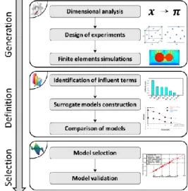
three main steps: data generation, surrogate model definition and surrogate model selection. Fig. 1 shows the global process of the methodology by presenting all the activities involved in each main step. A detailed description of the methodology is given in [8]. This methodology aims at facilitating the design of multi-physics systems and components by building surrogate models based on dimensional analysis and finite elements simulations.

Fig. 1: Procedure of the VPLM methodology Data generation

This step deals with the identification of the influent physical variables and the construction of the corresponding dimensionless numbers. Then, a design of experiments is used to define the configurations which have to be simulated by a finite element simulation software. The readers can follow the reference [11] for more details on design of experiments.

Surrogate model definition

This second step deals with the definition of the surrogate model, or in other words the algebraic expression of the model. As states the name of the methodology (VPLM), the chosen mathematical form of the model is a variable power law.

π0= 𝑘π1

𝑎₁(𝜋₁,𝜋₂,…,𝜋_𝑞−1)

π₂𝑎2(𝜋1,𝜋2,…,𝜋𝑞−1)

… π_𝑞−1𝑎𝑞−1(𝜋1,𝜋2,…,𝜋𝑞−1) (3) where 𝑎_𝑖(𝜋_𝑖, … , 𝜋_𝑞−1) are polynomial functions of log⁡(𝜋𝑖). In order to define the functions

𝑎𝑖(𝜋𝑖, … , 𝜋𝑞−1), a sensitivity analysis is conducted

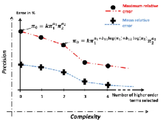
using the simulation data gathered during the first step. Several candidate models are built for which the relative errors and/or the standard deviation can be evaluated. In order to appreciate and compare the accuracy of the surrogate models built during the second step, the evolution of the relative errors

of each model (differing in the number of selected higher order terms) are shown in Fig. 2.

Fig. 2: Example of relative errors comparison between different models

Surrogate model selection

This third step of the VPLM methodology concerns the selection of the appropriate model and its validation regarding its accuracy and complexity. The engineer can make a compromise between accuracy and simplicity of the expected surrogate model. Thus, by looking at Fig. 2, it can be seen that the prediction accuracy increases with the number of selected terms, but the model becomes more bulky as well.

3. T

3.1. PROBLEM STATEMENT

The preliminary design of power converters requires mastering the thermal performances of somes electronic components. Thus it is necessary to have accurate thermal models since early design stage. The methodology described in this paper enables to generate thermal models in accordance with the requirements. The studied system is based on a prototype designed by ARCEL (Fig. 3).

Fig. 3 : DC/AC (one phase) converter prototype It is proposed here to generate the thermal model of a film capacitor used for filtering and the thermal model of the heatsink used to cool the IGBT modules.

3.2. THERMAL MODEL OF A FİLM CAPACİTOR

The life expectancy of capacitors highly depends upon their operating temperature [12]. Thus the evaluation of its thermal resistance is required. Due to its geometrical integration on the converter, the capacitor dissipates the generated losses through all the three heat transfer modes (conduction, convection and radiation). Indeed, for this geometry, semi-empirical laws [13] are available for each heat transfer mode. But, in order to use them we need to establish a nodal model including at least three nodes, i.e. the hot-spot, the case surface and the surrounding air. Generally, for the preliminary design of capacitors a straight forward relation that estimates the equivalent thermal resistance between the hot-spot and the ambient temperature is preferable. The VPLM methodology enables to build such model from finite element simulations.

It is considered that the capacitor is fixed on the printed circuit board through its terminals and the heat losses dissipated through them can be neglected. Natural convection cooling is considered and there is two assumptions (Fig. 4):

 Geometrical simplification: axi-symmetry hypothesis.

 Material simplification: an equivalent homogenized material (function of physical and geometrical characteristics of the layers) is modeling all the dielectric and electrode layers. This material has different physical properties for radial 𝜆𝑟 and axial 𝜆𝑧 directions.

Fig. 4 : Simplifying assumptions for film capacitor detailed thermal modeling

Two types of losses are considered for the thermal modelling: Joules losses dissipated in the conductors and dielectric losses dissipated in the dielectric layers. For the finite elements simulations these losses are generated in the equivalent material.

The thermal model of the capacitor is built by following the steps of the VPLM methodology: Data generation

The dimensional analysis shows that the problem depends on eleven physical quantities (4) and can be reduced to seven dimensionless numbers (5):

𝑅𝑡ℎ= 𝑓(𝑔βΔθ, λ, μ, Cp, 𝐷, 𝐿, 𝜆𝑟, 𝜆𝑧, 𝜌, 𝜀𝜎𝑇𝑎) (4)

𝜋0= 𝐹(𝐺𝑟, 𝜋2, 𝑃𝑟, 𝜋4, 𝜋5, 𝜋6) (5) where the dimensionless numbers are: the non-dimensional thermal resistance, 𝜋₀= 𝜆𝐷𝑅_𝑡ℎ; the modified Grashof number (expressed in term of heat flux),⁡𝐺𝑟 =𝜌2𝑔𝛽φ𝐷_𝜇2𝜆 4; the aspect ratio of the capacitor, 𝜋2=𝐷_𝐿; the Prandtl number, 𝑃𝑟 =𝜇𝜆_𝐶

𝑝; the thermal conductivities ratio, 𝜋4=𝜆_𝜆𝑟 and 𝜋5=𝜆_𝜆𝑧;

and the radiative dimensionless number, 𝜋₆=

𝜌2_𝐷3_𝜀σTa4

𝜇3 .The air properties are assumed to be constant and evaluated at the mean temperature. In addition, the radial thermal conductivity 𝜆𝑟 does not

change with the geometrical characteristics of the layers. Thus the Prandtl number and the dimensionless number 𝜋4 are constants and the

problem depends only on five dimensionless numbers.

A design of experiments of 81 points is built to define the configurations which have to be simulated by a finite elements model. The finite element model of the capacitor is built in COMSOL Multiphysics software.

Fig. 5 : Finite elements simulations results for diffferent capacitor geometry (left: 𝐷/𝐿 < 1, right:

𝐷/𝐿 > 1, temperature scale in °K) Surrogate model definition and selection

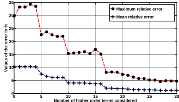
From the simulations results all the possible VPLM models are built and the evolution of the relative errors is represented in function of the complexity of the considered model (Fig. 6). During preliminary design stage, a model with less than 15% of maximum relative error remains acceptable. Thus the model (6) with ten higher order terms represents the best compromise between the expected accuracy and the complexity of the mathematical expression.

Fig. 6 : Evolution of the relative errors for different models of the capacitor

𝜋0= 0.039𝐺𝑟𝑎1(𝐺𝑟,𝜋2,𝜋5)𝜋2𝑎2(𝐺𝑟,𝜋2,𝜋5 ) × 𝜋₄𝑎4(𝐺𝑟,𝜋5)_𝜋 5𝑎5(𝐺𝑟,𝜋2,𝜋4,𝜋5 ) (6) 𝑎1= −0.335 − 1.27 ∙ 10−2𝑙𝑜𝑔(𝜋5)𝑙𝑜𝑔(𝐺𝑟) + 7.58 ∙ 10−3_{𝑙𝑜𝑔(𝐺𝑟)𝑙𝑜𝑔(𝐺𝑟)} + 1.26 ∙ 10−2_{𝑙𝑜𝑔(𝐺𝑟)𝑙𝑜𝑔(𝜋} 2) 𝑎2= −0.745 − 1.07 ∙ 10−2𝑙𝑜𝑔(𝜋5)𝑙𝑜𝑔(𝐺𝑟) − 0.378𝑙𝑜𝑔(𝜋2) 𝑎4= 0.234 − 1.62 ∙ 10−3𝑙𝑜𝑔(𝜋5)𝑙𝑜𝑔(𝐺𝑟) 𝑎5= 0.176 + 8.81 ∙ 10−3𝑙𝑜𝑔(𝜋5)𝑙𝑜𝑔(𝐺𝑟) − 2.26 ∙ 10−3_{𝑙𝑜𝑔(𝜋} 5)𝑙𝑜𝑔(𝜋5) + 3.25𝑙𝑜𝑔(𝜋5)𝑙𝑜𝑔(𝜋3) − 1.33 ∙ 10−3_{𝑙𝑜𝑔(𝜋} 5)𝑙𝑜𝑔(𝜋4)

Surrogate model validation

The prediction capability of the selected model is assessed by cross validation, which is illustrated on a scatter plot in Fig. 7.

Fig. 7 : Validation of the capacitor thermal model 3.3. THERMAL MODELLİNG OF A HEATSİNK

In the previous section was built a thermal model of a film capacitor cooled by natural convection. This cooling configuration is often insufficient for high power electronic components such as IGBT modules. A solution to improve the cooling performances of IGBT is to use a heatsink (Fig. 3). For the selection of this type of heatsink two physical parameters are important: the pressure drop through the heatsink and its thermal resistance. In this study a rectangular heatsink is considered cooled by a single fan.

0 5 10 15 20 25 30 0 5 10 15 20 25 30 35 V a lu e s o f th e e rr o r in %

Number of higher order terms considered Maximum relative error Mean relative error

0 0.01 0.02 0.03 0.04 0.05 0 0.01 0.02 0.03 0.04 0.05

Results from finite elements simulations

Es ti m a ti o n s fr o m th e s u rr o g a te m o d e l Building DoE Max error : 15.3 % Mean error : 4.0 % Cross validation DoE Max error : 19.7 % Mean error : 4.9 % y=x

Data generation

The dimensional analysis shows that the problem depends on twelve physical quantities (7) and can be reduced to eight dimensionless numbers:

𝑅𝑡ℎ

= 𝑓(ΔP, 𝜇, 𝜌, 𝜆, 𝐶𝑝, 𝑊ℎ, 𝐿ℎ, 𝑊𝑝, 𝑒𝑓, 𝐻𝑏, 𝑊𝑓) (7)

𝜋0= 𝐹(𝐵𝑒, 𝑃𝑟, 𝜋3, 𝜋4, 𝜋5, 𝜋6, 𝜋7) (8) where the dimensionless numbers are: the non-dimensional thermal resistance, 𝜋0= 𝜆𝐷𝑅𝑡ℎ; the

Bejan number, 𝐵𝑒 =Δ𝑃𝜌𝐿ℎ 2

𝜇2 ; the Prandtl number, 𝑃𝑟 =𝜇𝜆_𝐶 𝑝; geometrical ratios,⁡𝜋3= 𝑊_ℎ 𝐿ℎ, 𝜋4= 𝑒_𝑓 𝐿ℎ, 𝜋5= 𝑊_𝑝 𝐿ℎ, 𝜋6= 𝑊_𝑓 𝐿ℎ and 𝜋7= 𝐻_𝑏 𝐿ℎ.

As previously, the air properties are assumed to be constant and are evaluated at the mean temperature implying constant Prandtl number. Additionally, in order to reduce the number of parameters, two geometrical simplifications are made: the geometrical ratio between the height of the heatsink base (𝐻𝑏) and its length (𝐿ℎ) is kept constant; the

thickness of the fins (𝑊𝑓) is equal to the space

between the fins (𝑒𝑓). Thus, the dimensionless

numbers 𝜋₇ is constant and the dimensionless numbers 𝜋4 and 𝜋6 are equal. Considering all these

assumptions, the problem depends only on five dimensionless numbers: 𝐵𝑒, 𝜋3, 𝜋4 and 𝜋5.

A design of experiments of 81 points is built to define the configurations which have to be simulated by finite elements model in COMSOL Multiphysics software. The boundary conditions used for the simulations are:

 A pressure drop (Δ𝑃) is applied between the inlet and the outlet of the heatsink.

 A heat flux density of 2 ∙ 105⁡𝑊/𝑚2 is dissipated on a square surface (𝑆 = 𝑊𝑝2)

representing the IGBT module.

 The inlet temperature is equal to 300⁡°𝐾 and the heatsink does not exchange heat through its external surfaces.

Fig. 8 : Finite elements simulation results for the heatsink model (Temperature scale in °K) Surrogate model definition and selection

The results of the VPLM methodology (Fig. 9) show that the model with four higher order (9) terms seems to be the best compromise between accuracy and complexity.

𝜋0= 4.47 ∙ 10−4𝐵𝑒−0.024

× 𝜋₅−0.799+0.309 𝑙𝑜𝑔(𝜋2) 𝑙𝑜𝑔(𝜋2)

× 𝜋3−1.768+0.142 𝑙𝑜𝑔(𝐵𝑒)+1.133 𝑙𝑜𝑔(𝜋3)−0.357 𝑙𝑜𝑔(𝜋5)

× 𝜋40.515+0.163 𝑙𝑜𝑔(𝜋4)

(9)

Fig. 9 : Evolution of relative errors for different models of the heatsink

Surrogate model validation

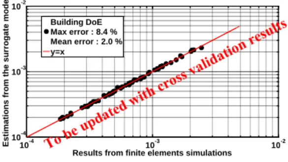
The prediction capability of the selected VPLM model is assessed by cross validation, which is illustrated on a scatter plot in Fig. 10.

Fig. 10 : Validation of the heatsink thermal model

4. P

The use of VPLM enables to reduce nodal network models composed of non-linear resistances (depending on the temperature, for example) of a capacitor (Fig. 11). Thus it allows linking directly the hot-spot temperature of the capacitor to the ambient temperature without estimating the case temperature. 0 5 10 15 20 25 30 0 5 10 15 20 Va lu es o f th e er ro r in %

Number of higher order terms considered

Maximum relative error Mean relative error

Air flow direction

10-4 10-3 10-2

10-4

10-3

10-2

Results from finite elements simulations

Es ti m a ti o n s fr o m th e s u rr o g a te m o d e l Building DoE Max error : 8.4 % Mean error : 2.0 % y=x

Fig. 11 : Nodal network representations of the thermal model of a capacitor: classical (top) and

proposed representations (bottom)

Another possible use of these models is their association to conduct the preliminary design of a system (the models are function of the geometry and some physical properties) or to investigate other cooling configurations for a component. For example, it is possible to evaluate the cooling capabilities of the capacitor if a heatsink is used (Fig. 12).

Fig. 12 : Nodal network representation for the association of models

5. C

This paper presented and applied a methodology for building algebraic thermal models of electronic components from finite elements simulations.The models of the components obtained by this method are modular and re-usable for different engineering problems and different systems involving these components. Finally it is shown that this type of models permits to simplify nodal network approach by reducing the numbers of required thermal resistances. I. Nomenclature 𝑅𝑡ℎ,𝑐 Thermal resistance of the capacitor, 𝐾/𝑊 𝐿 Length of the capacitor, 𝑚

𝑔 _{acceleration, 𝑚/𝑠}Gravitational 2 𝜌 Density of air, _{𝑘𝑔/𝑚}3

𝛽 Thermal expansion _{coefficient, 1/𝐾} 𝜀 Emissivity of _{the capacitor}

Δ𝜃 _{temperature, 𝐾} Elevation of 𝜎

Stefan-Boltzmann

constant, 𝑊/𝑚2_/𝐾4

𝜆 conductivity of air, Thermal 𝑊/𝑚/𝐾 𝑇𝑎

Ambient temperature, 𝐾

𝜇 Dynamic viscosity _{of air, 𝑘𝑔/𝑚/𝑠} 𝜑 _{density, 𝑊/𝑚}Heat flux 2

𝐶𝑝 Heat capacity of _{air, 𝐽/𝑘𝑔/𝐾} Δ𝑃 Pressure drop, _𝑃𝑎

𝐷 Diameter of the _{capacitor, 𝑚} 𝑊𝑓 Width of the _{fins, 𝑚}

𝑊ℎ Width of the _{heatsink, 𝑚} 𝑊𝑝 Width of the _{chip, 𝑚}

𝐿ℎ Length of the _{heatsink,⁡𝑚} 𝐻𝑏

Height of the heatsink base,

𝑚

𝑒𝑓 Space between the _{fins, 𝑚}

R

[1] P. Cova, N. Delmonte, and R. Menozzi, “Microelectronics Reliability Thermal modeling of high frequency DC – DC switching modules : Electromagnetic and thermal simulation of magnetic components,” Microelectron. Reliab., vol. 48, pp. 1468–1472, 2008.

[2] P. Cova and N. Delmonte, “Thermal modeling and design of power converters with tight thermal constraints,” Microelectron. Reliab., vol. 52, no. 9–10, pp. 2391–2396, Sep. 2012. [3] Aldo Boglietti, Andrea Cavagnino, David

Staton, Martin Shanel, Markus Mueller, and Carlos Mejuto, “Evolution and Modern Approaches for Thermal Analysis of Electrical Machines,” IEEE Trans. Ind. Electron., vol. 56, no. 3, pp. 871–882, 2009.

[4] T. Verstraten, G. Mathijssen, R. Furnémont, B. Vanderborght, and D. Lefeber, “Modeling and design of geared DC motors for energy efficiency: Comparison between theory and experiments,” Mechatronics, vol. 30, pp. 198– 213, 2015.

[5] C. Gogu, R. T. Haftka, S. K. Bapanapalli, and B. V. Sankar, “Dimensionality Reduction Approach for Response Surface Approximations: Application to Thermal Design,” AIAA J., vol. 47, no. 7, pp. 1700–1708, Jul. 2009.

[6] A. I. J. Forrester, A. Sóbester, and A. J. Keane,

Engineering Design via Surrogate Modelling.

2008.

[7] G. A. Vignaux and J. L. Scott, “Simplifying regression models using dimensional analysis,”

Austral. New Zeal. J. Stat., vol. 41, no. 1, pp.

31–41, 1999.

[8] F. Sanchez, M. Budinger, and I. Hazyuk, “Dimensional analysis and surrogate models for the thermal modeling of Multiphysics systems,”

Appl. Therm. Eng., vol. 110, pp. 758–771, Jan.

2017.

[9] E. Buckingham, “On physically similar systems: illustration of the use of dimensional equations,”

Phys. Rev., vol. 4, no. 4, pp. 345–376, 1914.

[10] T. Szirtes and P. Rózsa, Applied Dimensional

Analysis and Modeling. 2007.

[11] D. C. Montgomery, Design and Analysis of

Experiments, Eighth Edi. 2012.

[12] S. G. Parler, “Thermal Modeling of Aluminum Electrolytic Capacitor,” in IEEE, 1999, pp. 2418–2429.

[13] F. P. Incropera, D. P. DeWitt, T. L. Bergman, and A. S. Lavine, Fundamentals of Heat and

Mass Transfer, vol. 6th. John Wiley & Sons,