HAL Id: hal-00714553
https://hal.archives-ouvertes.fr/hal-00714553
Submitted on 5 Jul 2012
HAL is a multi-disciplinary open access
archive for the deposit and dissemination of sci-entific research documents, whether they are pub-lished or not. The documents may come from teaching and research institutions in France or
L’archive ouverte pluridisciplinaire HAL, est destinée au dépôt et à la diffusion de documents scientifiques de niveau recherche, publiés ou non, émanant des établissements d’enseignement et de recherche français ou étrangers, des laboratoires
Simulated Annealing, Wafer fabrication
Claude Yugma, Stephane Dauzere-Peres, Christian Artigues, Alexandre
Derreumaux, Olivier Sibille
To cite this version:
Claude Yugma, Stephane Dauzere-Peres, Christian Artigues, Alexandre Derreumaux, Olivier Sibille. Batching, Scheduling, Disjunctive graph, Local search, Simulated Annealing, Wafer fabrication. In-ternational Journal of Production Research, Taylor & Francis, 2011, �10.1080/00207543.2011.575090�. �hal-00714553�
For Peer Review Only
Batching, Scheduling, Disjunctive graph, Local search, Simulated Annealing, Wafer fabrication
Journal: International Journal of Production Research Manuscript ID: TPRS-2010-IJPR-0566.R1
Manuscript Type: Original Manuscript Date Submitted by the
Author: 11-Jan-2011
Complete List of Authors: Yugma, Claude; Ecolde des Mines de Saint-Etienne, CMPGC Dauzere-Peres, Stephane; Ecole des Mines de Saint-Etienne, CMP Georges Charpak
Artigues, Christian; Université de Toulouse, LAAS-CNRS
Derreumaux, Alexandre; Ecole des Mines de Saint-Etienne, CMP Georges Charpak
Sibille, Olivier; Zone industrielle d'ATMEL
Keywords: BATCH SCHEDULING, SCHEDULING, HEURISTICS,
SEMICONDUCTOR MANUFACTURE, SIMULATED ANNEALING Keywords (user):
For Peer Review Only
International Journal of Production Research Vol. 00, No. 00, 00 Month 200x, 1–21
RESEARCH ARTICLE
A Batching and Scheduling Algorithm for the Diffusion
Area in Semiconductor Manufacturing
Claude Yugma1∗, St´ephane Dauz`ere-P´er`es1, Christian Artigues2,3,
Alexandre Derreumaux1, Olivier Sibille4
1Ecole des Mines de Saint-Etienne, Centre Micro´´ electronique de Provence - Site
Georges Charpak, 880, Avenue de Mimet, F-13541 Gardanne, France
2CNRS, LAAS, 7 avenue du Colonel Roche, F-31077 Toulouse, France 3Universit´e de Toulouse, UPS, INSA, INP, ISAE, LAAS, F-31077 Toulouse,
France
4ATMEL, Zone industrielle, 13790 Rousset, France
(Received 00 Month 200x; final version received 00 Month 200x) This paper proposes an efficient heuristic algorithm for solving a complex batching and scheduling problem in a diffusion area of a semiconductor plant. Diffusion is frequently bottleneck in the plant and also one of the most com-plex areas in terms of number of machines, constraints to satisfy and the large number of lots to manage. The purpose of this study is to investigate an ap-proach to group lots in batches and to schedule these batches on machines. The problem is modeled and solved using a disjunctive graph representation. A constructive algorithm is proposed and improvement procedures based on iterative sampling and Simulated Annealing are developed. Computational ex-periments, carried out on actual industrial problem instances, show the ability of the iterative sampling algorithms to significantly improve the initial solu-tion, and that Simulated Annealing enhances the results. Furthermore, our algorithm compares favorably to an algorithm of the literature on a simplified version of our problem. The constructive algorithm has been embedded in a software and is currently being used in a semiconductor plant.
Keywords: Batching, Scheduling, Disjunctive graph, Local search, Simulated Annealing, Wafer fabrication
1. Introduction
Semiconductor wafer fabrication can be described as a multistage process with re-entrant flows. The processing is done layer by layer. Each layer requires several steps of
process-∗Corresponding author. Email: [email protected]
1 2 3 4 5 6 7 8 9 10 11 12 13 14 15 16 17 18 19 20 21 22 23 24 25 26 27 28 29 30 31 32 33 34 35 36 37 38 39 40 41 42 43 44 45 46 47 48 49 50 51 52 53 54 55 56 57 58 59 60
For Peer Review Only
ing such as chemical-mechanical polishing, diffusion, film deposition, photolithography, implant (doping) and etching. For each of the product types, and depending on the tech-nology, a wafer goes through more than 400 process steps over a period of a few weeks. Wafer fabrication planning and scheduling is a complex task due to the large number of products and machines involved. It is further complicated by additional constraints such as re-entrant flow of operations (see (Kumar 1994)), setup issues, preventive mainte-nances and random machine breakdowns (see (Ovacik and Uzsoy 2007) and (Sze 2001)). The importance of scheduling on the performance of semiconductor wafer fabrication facilities (fabs) is known for many years (see (Wein 1988) and (Varadarajan and Sarin 2006)).
In this paper, we focus on an important part of the manufacturing process. Among the complex operations involved in the fabrication of a wafer, the diffusion phase is of critical importance since the batching decisions that are involved may affect the perfor-mance of the entire wafer fab (see for instance (Ibrahim et al. 2003) and (Monch and Habenicht 2003)). The processing time of the operations in the diffusion area can be large (10 hours) compared to other operations in the fab. (Mehta and Uzsoy 1998) state that optimizing batching operations results in good performance measures of the whole production process. Lots regularly arrive in the diffusion area and the diffusion phase is primarily used to alter the type and level of conductivity of semiconductor materials.
The purpose of this article is to develop efficient methods to partition lots in batches and to schedule batches on machines in the diffusion area while taking into account numerous constraints and optimizing three main production criteria: maximizing the number of operations (moves), maximizing the batch sizes and minimizing the total tardiness.
The remaining sections of this paper are organized as follows. In Section 2, we provide some background on existing related batching and scheduling problems. In Section 3, the problem is stated. We present in Section 4 a disjunctive graph representation of the problem, which supports our solving procedures. The method for computing an initial solution and improvement procedures based on iterative sampling and Simulated Annealing are described in Section 5. Experimental results on real problem instances and comparison with an algorithm of the literature are given and discussed in Section 6. Section 7 concludes the paper with recommendations for further research.
2. Previous related work
The operations of batching and scheduling jobs are a common practice in manufactur-ing systems, especially in semiconductor manufacturmanufactur-ing systems, see (Mathirajan and Sivakumar 2006a) for more details. Reasons for batching are the reduction of setups, the ability of machines to process several jobs simultaneously, etc. Using the classification of (Mathirajan and Sivakumar 2006a), we notice that there is not much literature on batch scheduling problems taking into account the re-entrance features of the system, see for examples (Cigolini et al. 2002), (Mason and Oey 2003) and (Oey and Mason 2001).
(M¨onch et al. 2009) present a survey on scheduling problems in semiconductor
manu-facturing, where typical batching problems are described. For a general introduction on scheduling problems, the reader can for instance refer to (Blazewicz et al. 2007).
The problem addressed in this paper deals with the following characteristics:
• Multiple non-identical machines at each stage. (Mehta and Uzsoy 1998) present a to-tal tardiness minimization problem on a batch processing machine with incompatible
4 5 6 7 8 9 10 11 12 13 14 15 16 17 18 19 20 21 22 23 24 25 26 27 28 29 30 31 32 33 34 35 36 37 38 39 40 41 42 43 44 45 46 47 48 49 50 51 52 53 54 55 56 57 58 59 60
For Peer Review Only
job families. They propose a dynamic programming algorithm to solve the problem. (Balasubramanian et al. 2004) extend the approach of (Mehta and Uzsoy 1998) to a batching problem with incompatible jobs on parallel machines aiming at minimizing the weighted total tardiness. The main focus of interest in (Kim et al. 2010) is the scheduling of lots on diffusion workstations in a fab. There are multiple identical ma-chines, and each of them can process a limited number of lots at a time. The scheduling problem involves multiple job families on identical parallel batch-processing machines. • Multiple stages. Jobs have to be processed on a cleaning machine in a first stage, and then on furnaces in a second stage. The second stage is actually a multi-stage process, since jobs may have up to three different consecutive operations on furnaces. Moreover, the sequence of operations can differ from one job to another depending of the type of operations that the jobs must undergo. For example, the same furnace can be used for the last furnace operation for a job in a batch and for the first furnace operation for another job in another batch. Our problem is thus different from a flexible flow-shop scheduling problem (see (Kis and Pesch 2005)), where the processing order is the same for all jobs. In the literature, the number of stages usually does not exceed two. (Su 2003) considers an hybrid two-stage flow-shop scheduling problem with a batch processor in Stage 1 and a single processor in Stage 2. This is also the case in (Sung and Min 2001) and (Sung and Kim 2003) where a batching problem on two stages is considered. (Oulamara et al. 2009) study a two-machine flow-shop scheduling problem with conventional and batching machines in the first and second stage, respectively, and arbitrary job compatibilities.
• Multiple criteria. The goal of the paper is to simultaneously optimize three indicators. These indicators are the number of wafers going through the line (to maximize), the average number of lots in batches (to maximize) and the waiting time of lots (to minimize). Generally, related studies in the literature tackle scheduling problems by considering one single indicator to optimize. (Uzsoy 1995) tackles the problem with the objective of minimizing the completion time of jobs, and (Hung 1998) the objective of maximizing the batch processing machine utilization. The minimization of the total weighted tardiness on a single machine is considered in (Perez et al. 2005) while, in (Mathirajan and Sivakumar 2006b), the authors focus on the minimization of the total weighted tardiness on heterogeneous batch processing machines under dynamic arrival of jobs, incompatible job families and non-identical job sizes. Few articles deal with different criteria simultaneously. In (Pfund et al. 2008), the authors adapt the Shifting Bottleneck Heuristic to facilitate the multi-criteria optimization of makespan, cycle time and total weighted tardiness using a desirability function.
Furthermore, in our problem, there are setup times (corresponding to loading and un-loading lots from the machine), which do not depend on the sequence, and the complexity is increased by the presence of maximum times lags between batching operations.
Our problem can be viewed as a complex variant of the flexible job-shop scheduling
problem (see for instance (Dauz`ere-P´er`es and Paulli 1997)). These types of problems
have been addressed by several authors, as in (Mason et al. 2002) and (Ovacik and Uz-soy 2007). These problems are frequently solved using a method known as the Shifting Bottleneck (SB) procedure originally designed for the standard job-shop scheduling
prob-lem (see (Adams et al. 1988) and (Dauz`ere-P´er`es and Lasserre 1993)). Several aspects,
like identifying appropriate subproblem solution procedures, can be found in (Demirkol and Uzsoy 2000) and (Uzsoy and Wang 2000). In (Mason et al. 2002), a scheduling prob-lem in semiconductor manufacturing close to the one tackled in this paper is solved by a modified Shifting Bottleneck heuristic. We model the considered batching and scheduling
1 2 3 4 5 6 7 8 9 10 11 12 13 14 15 16 17 18 19 20 21 22 23 24 25 26 27 28 29 30 31 32 33 34 35 36 37 38 39 40 41 42 43 44 45 46 47 48 49 50 51 52 53 54 55 56 57 58 59 60
For Peer Review Only
problem through a variant of the disjunctive graph described in (Mason et al. 2002), and we use it to propose different solving procedures.
3. Problem description
The diffusion area defines a batching and scheduling problem of wafer lots on two types of equipment: cleaning machines and furnaces. These resources are able to perform several lots simultaneously. Each lot requires one or more consecutive operations in the diffusion
area, and each operation has a recipe1 which determines its duration and the set of
machines that are able to process the lot. On a 24-hour basis, each operation has to be assigned to a machine and included into a batch, i.e. a set of operations of the same recipe that are simultaneously processed by the machine. Lots usually have to be processed on one cleaning machine and then on one or more furnaces. Constraints in the diffusion area are divided into three types: Equipment constraints, process constraints and line management constraints.
3.1. Constraints
Some of these constraints are common to the two types of resources while others are dedicated to furnaces.
3.1.1. Equipment constraints
• Common constraints
Dedicated equipment : Any machine is able to process a limited set of recipes.
Maximum batch size: Any machine defines a maximum batch size corresponding to its capacity.
Loading and unloading times: A time may be needed to load and unload a batch on the machine.
Unavailability periods: The machine may be unavailable during some periods (defined by time windows) due to qualification, repair, maintenance, etc.
In process jobs: The machine may be occupied at the beginning of the time horizon by in-process operations that have to be completed before the machine becomes available. • Specific furnace constraints
Minimum time between two batches on an furnace: Furnaces must be inspected after completing each batch.
3.1.2. Process constraints
• Common constraints
Precedence: Operations must be performed following the manufacturing process of the lot. The operations of a lot are chained and no operation can start before the end of its predecessor, except for the first operation of each lot.
Minimum time lag: There is a fixed handling and transport time between every two successive operations of a lot.
Release dates: They correspond to the arrival times of lots at the cleaning machines and furnaces. A lot cannot be scheduled before its release date. Because the diffusion
1Specifications on a process on how it should be executed on a tool; This pertains to requirements of maintaining
proper temperature, pressure, and metal composition, among others. 4 5 6 7 8 9 10 11 12 13 14 15 16 17 18 19 20 21 22 23 24 25 26 27 28 29 30 31 32 33 34 35 36 37 38 39 40 41 42 43 44 45 46 47 48 49 50 51 52 53 54 55 56 57 58 59 60
For Peer Review Only
area is a stage of the complex global production process, release dates are estimated by a simulation tool.
Fixed recipe: Each operation of a lot is associated with a recipe, i.e. the lot should be processed on resources that are qualified for the corresponding recipe. This implies that all lots in the same batch must be processed with the same recipe.
Process time: The process time of a batch on a machine depends on the recipe. maximum time lag: A time limit is given for two successive operations x and y of a lot. The difference between the starting time of y and the completion time of x cannot exceed this limit. The maximum time lag depends on the operations x and y and corresponds, for instance, to the maximum time allowed between a cleaning operation and the first operation on a furnace.
3.1.3. Line management constraints
• Specific furnace constraints
Minimum time between two batches of the same recipe: There is a minimum time between the beginning of two batches of the same recipe on two different furnaces.
3.2. Objective
In semiconductor fabs, several indicators are used to measure the performance. The inter-ested reader can refer to (Montoya-Torres 2006) for more details. Jointly with managers of the fab, we identified three relevant indicators for our study, that are described below. • Number of moves (to maximize). It corresponds to the number of completed operations on the planning horizon, which can be compared to the target number fixed by the production managers.
• Batching coefficient (to maximize). Defined on the planning horizon, it is calculated as the number of moves divided by the sum of the number of batches performed on each machine, times the maximum capacity of that machine. Note that the denominator is the number of lots that could be performed if the machine was loaded up to its maximum capacity.
• X-factor (to minimize). This indicator is used to evaluate the waiting times of lots in the diffusion area in order to reduce cycle times. For a given lot, this factor is calculated as the total time of the lot in the diffusion area over its processing time.
It must be noted that these indicators are not always antagonist, e.g. increasing the batching coefficient usually leads to increasing the number of moves. However, each indicator shows a different aspect of a proposed schedule to managers. Depending on the situation in the fab, it might be preferable to prioritize the maximization of the batching coefficient, which may lead to an increased X-factor, since some lots might wait for other lots of the same family to arrive in the diffusion area to create a larger batch.
In the literature, although other indicators are used to evaluate the quality of a solution, we can show that they are equivalent to ours. The Work-In-Process (WIP) is defined as the number of wafers being in the fab at a given period, either in a production state or in a non-production state (e.g. transport and waiting). Little’s law (Little 1961) establishes that, if a system is stable and stationary, then the average WIP is proportional to the average cycle time. The WIP indicator is linked to the X-factor. The throughput, defined as the outgoing number of wafers of the fab per unit of time, is linked to the number of moves. The evolution of the throughput in time makes it possible to know if the system is stable, i.e. to know if there is no accumulation of lots in the fab or if the
1 2 3 4 5 6 7 8 9 10 11 12 13 14 15 16 17 18 19 20 21 22 23 24 25 26 27 28 29 30 31 32 33 34 35 36 37 38 39 40 41 42 43 44 45 46 47 48 49 50 51 52 53 54 55 56 57 58 59 60
For Peer Review Only
system evolves according to forecasts. (Glassey and Resende 1988) observe that there is a relation between the increase of the throughput and the output of a fab. The cycle time drastically increases when the throughput is close to the maximal capacity of the fab. Hence, to consider both WIP and throughput, our indicators are adequate.
The goal is to optimize the various performance measures, while taking into account the numerous complex constraints. The next section describes the mathematical formulation of the problem.
3.3. Mathematical formulation of the problem
The scheduling problem can be formulated as follows. For sake of clarity, the above-described Unavailability periods, In-process jobs and Minimum distance between batches of the same recipe constraints are not included. In Section 4, we describe how we tackle these characteristics.
A set of jobs (lots) J = {Ji|i = 1, . . . , n} has to be processed on a horizon T by a
set of machines M = {Mk|k = 1, . . . , m}. Each job Ji is made of ni operations such
that each operation Oij has a duration pij > 0 and a set Mij ⊆ M of machines (the
furnaces or the cleaning machines) able to process it. Let Ok = {Oij ∈ O|Mk ∈ Mij}
denote the set of operations that can be assigned to machine Mk. The value of pij and
the elements of the set Mij are determined by the recipe of operation Oij denoted ρij. In
general we have Mij ⊂ M since each machine cannot be configured for all recipes. Each
operation Oij has to be included in a batch on a resource k ∈ Mij. Each machine has a
finite capacity Rk which gives the maximal number of lots in the same batch. On each
machine k, Skdenotes the setup time needed before starting a new batch, Dkdenotes the
removal time needed after the completion of a batch and sk denotes the constant setup
time needed between two different batches. s0k denotes the initial setup time on machine
k, depending on the state of the resource at time 0. Two consecutive operations Oij and
Oi(j+1) of the same job are linked by minimum and maximum time lags. Once the batch
of Oij is completed and removed from k, the setup for the batch of Oi(j+1) cannot start
before a minimum time lag τijmin and has to start before a maximum time lag τijmax. Let
O = {Oij|i = 1, . . . , n; j = 1, . . . , ni} denote the set of all operations. Each job Ji has a
relative priority ci (ci < cj means that Ji is more urgent than Jj). Each job corresponds
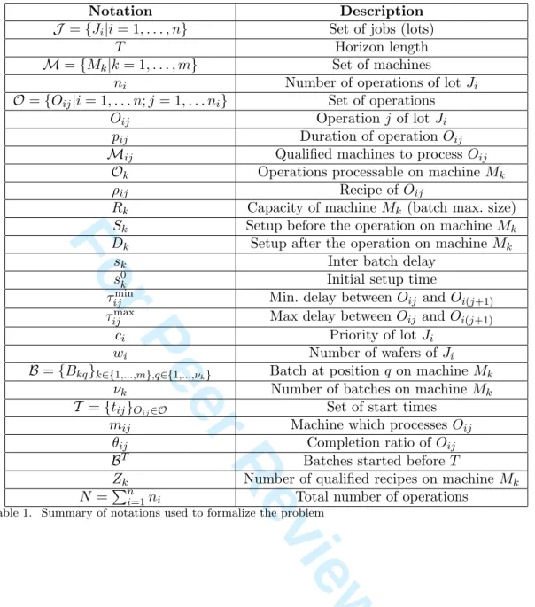
to a number wi of wafers produced when the job is completed. Table 1 summarizes the
notations.
Finding a feasible solution for the problem lies in making four types of decisions: D1 - Partition the operations into batches,
D2 - Select a resource to process each batch, D3 - Order the batches on each resource, D4 - Assign a start time to each batch.
Decisions D1-D3 can all be represented by a family of batches B =
{Bkq}k∈{1,...,m},q∈{1,...,νk} where Bkq is the batch sequenced at position q on machine
Mk. νk ∈ {0, . . . , |Ok|} denotes the number of batches assigned to machine Mk.
De-cision D4 leads to a family of start times T = {tij}Oij∈O assigned to the operations.
Once a solution {B, T } is determined, we have a machine assignment {mij}Oij∈O where
mij denotes the machine Oij is assigned to, i.e. verifying that ∃ q ∈ {1, . . . , νk} such
that Oij ∈ Bmijq. To be feasible, a solution {B, T } and its corresponding assignment
{mij}Oij∈O have to satisfy the following constraints. The operations of the same batch
4 5 6 7 8 9 10 11 12 13 14 15 16 17 18 19 20 21 22 23 24 25 26 27 28 29 30 31 32 33 34 35 36 37 38 39 40 41 42 43 44 45 46 47 48 49 50 51 52 53 54 55 56 57 58 59 60
For Peer Review Only
Notation Description
J = {Ji|i = 1, . . . , n} Set of jobs (lots)
T Horizon length
M = {Mk|k = 1, . . . , m} Set of machines
ni Number of operations of lot Ji
O = {Oij|i = 1, . . . n; j = 1, . . . ni} Set of operations
Oij Operation j of lot Ji
pij Duration of operation Oij
Mij Qualified machines to process Oij
Ok Operations processable on machine Mk
ρij Recipe of Oij
Rk Capacity of machine Mk (batch max. size)
Sk Setup before the operation on machine Mk
Dk Setup after the operation on machine Mk
sk Inter batch delay
s0k Initial setup time
τijmin Min. delay between Oij and Oi(j+1)
τmax
ij Max delay between Oij and Oi(j+1)
ci Priority of lot Ji
wi Number of wafers of Ji
B = {Bkq}k∈{1,...,m},q∈{1,...,νk} Batch at position q on machine Mk
νk Number of batches on machine Mk
T = {tij}Oij∈O Set of start times
mij Machine which processes Oij
θij Completion ratio of Oij
BT Batches started before T
Zk Number of qualified recipes on machine Mk
N =Pn
i=1ni Total number of operations
Table 1. Summary of notations used to formalize the problem
must have the same recipe, i.e.
ρij = ρxy ∀B ∈ B, ∀Oij, Oxy ∈ B (1)
Each operation must be assigned to a machine able to process its recipe:
mij ∈ Mij ∀Oij ∈ O (2)
The batch capacity cannot be exceeded and each batch includes at least one operation:
1 ≤ |Bkq| ≤ Rk ∀Bqk ∈ B (3)
An operation appears in only one batch, i.e.
B ∩ B0 = ∅ ∀B, B0 ∈ B, B 6= B0 (4) 1 2 3 4 5 6 7 8 9 10 11 12 13 14 15 16 17 18 19 20 21 22 23 24 25 26 27 28 29 30 31 32 33 34 35 36 37 38 39 40 41 42 43 44 45 46 47 48 49 50 51 52 53 54 55 56 57 58 59 60
For Peer Review Only
All operations are included in a batch:
∪B∈BB = O (5)
The start time of the first operation of each lot cannot exceed the lot release date:
ti1≥ ri ∀Ji∈ J (6)
Each operation Oij, j > 1, cannot start before a minimum time lag after the end of
its preceding operation Oi(j−1), which takes into account the removal time of the batch
of Oi(j−1), the minimum time lag τmin
i(j−1) and the setup time of the batch of Oij:
tij− ti(j−1) ≥ Dmi(j−1)+ pi(j−1)+ τ min
i(j−1)+ Smij ∀i ∈ {1, . . . , n}, ∀j ∈ {2, . . . , ni} (7)
Each operation Oij, j > 1, has to start before a maximum time lag after the end of its
preceding operation Oi(j−1), which takes into account the removal time of the batch of
Oi(j−1), the maximum time lag τi(j−1)max and the setup time of the batch of Oij:
tij− ti(j−1) ≤ Dmi(j−1)+ pi(j−1)+ τ max
i(j−1)+ Smij ∀i ∈ {1, . . . , n}, ∀j ∈ {2, . . . , ni} (8)
The start times of two operations of the same batch must be equal:
tij = txy ∀B ∈ B, ∀Oij, Oxy ∈ B (9)
An operation of a batch which is not at the first position on its machine cannot start before the end of the preceding batch on the machine, plus the necessary removal time of the preceding batch, plus the minimum setup time on the machine between two batches, plus the necessary setup time for the next batch.
tij − txy ≥ pxy+ Dk+ sk+ Sk ∀Bkq,q>1∈ B, ∀Oij ∈ Bkq, ∀Oxy ∈ Bk(q−1) (10)
An operation of a batch in the first position on its machine cannot start before the
initial setup time for this batch (we assume Sk0≤ Sk+ Dk+ sk, ∀Mk∈ M):
tij ≥ s0mij ∀Oij ∈ O (11)
By definition, a feasible solution includes each operation inside a batch. In our problem, the scheduling horizon is limited to T . Hence, only those batches released in the interval [0, T ] must be taken into account. Several criteria are used to measure the quality of a feasible solution. The number of moves is the number of wafers produced in [0, T ]:
fmov = X
Oij∈O
wiθij (12)
where wi is the number of wafers in job i (wi ≤ 25 in practice), and θij ∈ [0, 1] denotes
the completion ratio of operation Oij before time T , i.e.
θij = (min(t ij+pij,T )−tij pij if tij ≤ T 0 Otherwise. 4 5 6 7 8 9 10 11 12 13 14 15 16 17 18 19 20 21 22 23 24 25 26 27 28 29 30 31 32 33 34 35 36 37 38 39 40 41 42 43 44 45 46 47 48 49 50 51 52 53 54 55 56 57 58 59 60
For Peer Review Only
The batching coefficient is the average ratio of the actual size of each batch divided by
its maximal size. Let BT = {B ∈ B|tij < T, ∀Oij ∈ B} denote the set of batches started
before time T . Batching coefficient = P k P Bkq∈BT |Bkq|/Rk |BT| (13) fbatch = P k P Bkq∈BT|Bkq|/(Rk+ Zk 100) |BT| (14)
where Zk is the total number of qualified recipes on machine Mk.
The weighting of the batching coefficient by the number of qualified recipes on the concerned machine makes it possible to use the least general-purpose machines preferably. The average X-factor is the average of the X-factor of each job weighted by the job priority. All the jobs do not have the same priority. Some jobs are more important than others (important customers, tests to be carried out quickly, delay to catch up with,
etc). Thus, a weight ci is assigned to each job Ji to reflect its priority. Let JT = {Ji ∈
J |tini+ pini ≤ T } denote the set of jobs completed before T .
X-fac = P Ji∈JT(tini+ pini− ri)/pini |JT| (15) fX-fac = P Ji∈JT ci(tini+ pini− ri)/pini |JT| (16)
The choice made together with the decision makers of the production unit is to combine these different objectives into a single one by maximizing the following weighted sum:
f = αfmov + βfbatch − γfX-fac (17)
where α, β and γ are adjustable weights allocated to each objective function. The ob-jective functions have been designed to integrate some requests of managers. In the
calculation of fX−f ac, the delay of each lot is multiplied by its priority, in order to
ac-celerate the urgent lots. In the calculation of the total batching coefficient, the batching coefficient of each machine is multiplied according to the number of qualified recipes on this machine. This leads to choosing in priority the machines that are able to process less recipes, and thus to maintain the availability of the most flexible machine.
The objective of the problem is to determine a feasible selection {B, T } such that f is maximized. Note that, given a (feasible) solution {B, T }, f can be computed in O(N )
time where N =Pn
i=1ni is the total number of operations.
1 2 3 4 5 6 7 8 9 10 11 12 13 14 15 16 17 18 19 20 21 22 23 24 25 26 27 28 29 30 31 32 33 34 35 36 37 38 39 40 41 42 43 44 45 46 47 48 49 50 51 52 53 54 55 56 57 58 59 60
For Peer Review Only
4. The disjunctive graph representation
The considered problem can be seen as an extension of the flexible job-shop scheduling problem and, consequently, the disjunctive graph model can be used for this batching and scheduling problem as proposed in (Mason et al. 2002). In their article, the authors consider a different objective function (total weighted tardiness). Sequence-dependent setup times and reentrant flows are also considered but there are no maximum time lags. Unfortunately, these constraints considerably increase the difficulty of the problem (see (Gentner et al. 2004)). Let us explain how the problem is modeled using disjunctive graphs.
We define the disjunctive graph G = (V, C, E) as follows.
• V is a set of nodes where there is one node per operation, denoted Vij, plus a dummy
start node denoted 0.
• C is the set of conjunctive arcs representing the release dates and minimum and
max-imum time lags. There is an arc from node 0 to node Vi1 of each job Ji. There is an
arc from Vij to Vi(j+1) and an arc from Vi(j+1) to Vij, for pair of each consecutive
operations Oij and Oi(j+1) of each job Ji.
• E is the set of disjunctive arcs which represent the decisions of the problem. There
are two opposite conjunctive arcs (Vij, Vxv)k and (Vxy, Vij)k for any machine k ∈ M
and for any pair of operations Oij, Oxy ∈ Ok, Oij 6= Oxy. These arcs represent the
sequencing or the batching decision concerning Oij and Oxy on machine k.
Let B denote a partial or complete batching for the problem satisfying at least Con-straints (1) through (4). B is a complete batching if Constraint (5) is also verified,
oth-erwise it is a partial batching. Recall that B also defines the machine assignment mij,
for all Oij ∈ ∪B∈BB. We assume mij = 0 if Oij is not batched in B, i.e. if Oij 6∈ ∪B∈BB.
B unambiguously defines a selection S as follows. For each distinct operations Oij and
Oxy such that mij = mxy = k 6= 0, select arc (Vxy, Vij)k if Oxy is in a batch sequenced
before the batch of Oij, select arc (Vij, Vxy)k if Oij is in a batch sequenced before the
batch of Oxy, and select both arcs (Vij, Vxv)k and (Vxy, Vij)k if Oij and Oxy are assigned
to the same batch.
Once a selection is computed, we define a graph G(S) = (V, C ∪ S) where arcs C ∪ S
are valued as follows (we assume s00= s0 = S0 = D0= 0):
• Each arc from 0 to the first operation Oi1 is valued by max(ri, Sm0ij), the maximal
value between the release date of job i and the initial setup time for machine mi1.
• Each arc from Vij and Vi(j+1) is valued by Dmij+ pij+ τ
min
ij + Smi(j+1), the value of the
minimum time lag between Oij and Oi(j+1) plus the setup and removal times linked
to the assignment of the operations.
• Each arc from Oi(j+1)and Oij is valued by −(Dmij+pij+τ
max
ij +Smi(j+1)), the (negative)
value of the maximum time lag between Oij and Oi(j+1) plus the necessary setup and
removal times.
• Each arc (Vij, Vxv)kis valued either by pij+Dk+sk+Skif the opposite arc is not selected
or by 0 if the opposite arc is selected. Indeed, in the first case, this arc represents the
decision to sequence Oxy after Oij on machine k whereas, in the second case, both arcs
(Vij, Vxv)k and (Vxv, Vij)k represent the synchronization of the operations included in
the same batch.
We can state that the (partial) solution represented by the (partial) batching B and its
selection S is feasible if and only if all longest path problems from node 0 to each node Vij
4 5 6 7 8 9 10 11 12 13 14 15 16 17 18 19 20 21 22 23 24 25 26 27 28 29 30 31 32 33 34 35 36 37 38 39 40 41 42 43 44 45 46 47 48 49 50 51 52 53 54 55 56 57 58 59 60
For Peer Review Only
in G(S) have a solution. If this is the case and if B is complete, a feasible schedule T can
be obtained by setting tij to the length of the longest path from 0 to Vij. Furthermore, T
is the best schedule compatible with B one can obtain when the objective is to maximize f .
The problem can be formulated as follows: Find the batching B verifying Constraints (1) through (5) such that the corresponding selection S is feasible and maximizes f .
As stated in the previous sections, the actual data issued from the fab have other characteristics that have been tackled, such as in-process jobs and machine down times. Thanks to the disjunctive graph representation, we can model these two characteristics by operations with fixed start times on the machines. A start time t can be fixed by linking the node with node 0 by two opposite arcs valued by t and −t. As stated in Section 3, the actual problem also includes an important line management constraint: A minimum time between the start time of two batches of the same recipe scheduled on two different batches has to be respected. This can also be tackled through the disjunctive graph representation. A fictitious machine can be associated to each recipe, and disjunctive arcs linking two operations of the same recipe can be defined. Then, whenever the two operations are batched on two different machines (furnaces), the disjunctive arc has to be oriented. Once oriented, the arc is valued by the minimum required distance.
The disjunctive graph is extensively used in the solution methods proposed in the fol-lowing section. The graph is necessary to determine feasible solutions in the constructive algorithms, to evaluate solutions and also to move from one solution to another in the neighborhood of the Simulated Annealing algorithm.
5. Solution Methods
We propose a two-phase heuristic method and a metaheuristic to solve the problem. The first phase of the heuristic is a constructive heuristic based on successive job insertions. The second phase is a local search method which aims at improving the initial solution. Both phases are based on the evaluation of a (complete or partial) selection through the orientation of arcs and longest path calculations in the disjunctive graph. For the metaheuristic, we propose a Simulated Annealing algorithm with a neighborhood based on the graph representation.
5.1. Evaluation of a partial or complete batching
Any partial or complete batching B and its selection S can be evaluated through the
calculation of start times tij, equal to the longest path from 0 to Vij in G(S) of each
operation Oij. To compute such longest paths, since the graph includes arcs with negative
weights, we use the Bellman-Ford algorithm which has a O(N |S ∪ C|) time complexity. If the algorithm finds a path of positive length, then the partial or complete solution is
unfeasible. Otherwise the algorithm returns the start times tij, and the objective function
value f can be determined.
5.2. Computing an initial solution by a priority rule-based constructive heuristic
The initial solution (selection) is computed by a job insertion method. The jobs are first sorted in a list L according to the order: Jobs with increasing maximum time lags first,
1 2 3 4 5 6 7 8 9 10 11 12 13 14 15 16 17 18 19 20 21 22 23 24 25 26 27 28 29 30 31 32 33 34 35 36 37 38 39 40 41 42 43 44 45 46 47 48 49 50 51 52 53 54 55 56 57 58 59 60
For Peer Review Only
then increasing release dates, then job priorities.
The method starts with an empty batching. Then, the jobs are taken in the order
given by the list and inserted one by one in the current batching. The insertion of Ji
is made as follows. Let B = {Bkq}k∈M,q∈1,...,νk denote the current batching including
jobs located before Ji in L. For each operation Oij of Ji and for each resource k ∈ Mij,
there are 2νk+ 1 insertion positions of Oij in the batch sequence of machine Mk: Indeed,
for each batch Bkq, we may insert Oij inside batch Bkq or create a new batch at any
position. Each of these insertion positions is evaluated with the algorithm described in the previous section and the one that maximizes f is kept to update B. If none of the
insertion positions is feasible for an operation Oij, then all these partial solutions violate
a maximum time lag and there exist insertion positions that violate only the maximum
time lag between Oi(j−1)and Oij (the last position on each resource of Mij, for instance).
Hence, Oi(j−1), the previous operation of job Ji, has to be removed from B and inserted
at a later position. If this is not feasible, Oi(j−1)and Oij are not scheduled and are deleted
from the list of operations. We use the disjunctive graph for the sequence of operations and time lags (conjunctive arcs), batching (disjunctive arcs are created between jobs of the same batch) and batch sequences on the same tool. Bellman’s algorithm is used to calculate the start dates of operations and to detect infeasible solutions. Note that at
mostPni
j=1
P
k∈Mij2νk+ 1 insertion positions are tested per inserted lot. Thereafter, the
algorithm described above will be called Priority-rule Based Insertion Algorithm (PBIA).
5.3. Improving the initial solution by iterative sampling
As shown in the previous section, a solution can be computed with PBIA based on a list of jobs. Our first iterative sampling algorithm, called Pseudo-Random Iterative Algorithm by Priority-rule Based Insertion (PRIA-PBIA), consists in applying PBIA on a list that is only moderately changed compared to the list used in Section 5.2. This will be done by, when the list is constructed, randomly selecting a job in the set of jobs not already selected that are close regarding the ranking criteria (minimum maximum time lag remaining, minimum release date and maximum job priority). The goal is to only allow limited perturbations of the initial list.
On the contrary, in our second iterative sampling algorithm called Random Iterative Algorithm by Priority-rule Based Insertion (RIA-PBIA), PBIA is applied on a list of jobs that is entirely randomly constructed. Hence, any list of jobs can be generated. The interest of RIA-PBIA is that very different solutions can be attained. Numerical experiments in Section 6 show that, as expected, the quality of the solutions obtained with RIA-PBIA is very variable. However, better solutions than the ones obtained with PRIA-PBIA can sometimes be obtained.
5.4. Simulated Annealing
Simulated annealing (SA) belongs to the class of randomized local search algorithms and has been developed by (Kirkpatrick et al. 1983) to handle hard combinatorial problems. The use of simulated annealing supposes the definition of a neighborhood. Our neigh-borhood is based on the disjunctive graph representation and is defined by the following moves:
(1) ”Batch move”. A batch is randomly moved (both the machine and the position can change), 4 5 6 7 8 9 10 11 12 13 14 15 16 17 18 19 20 21 22 23 24 25 26 27 28 29 30 31 32 33 34 35 36 37 38 39 40 41 42 43 44 45 46 47 48 49 50 51 52 53 54 55 56 57 58 59 60
For Peer Review Only
(2) ”Operation move”. An operation is randomly moved in an existing batch or a new batch is created (both the machine and the position can change),
(3) ”Operation switch”. Two batches with the same recipe are randomly selected, and two randomly selected operations are switched.
In our implementation, 50% of the considered moves are batch moves, 25% are oper-ation moves and 25% are operoper-ation switches. According to randomly generated moves, we proceed as follows. All random selections are made according to the uniform law. If a move is impossible due to a constraint violation, we restore the previous solution and try another move. Each neighbor solution is evaluated by means of the longest path computations discussed in Section 5.1.
The algorithm starts with an initial solution s0, and then tries to find better solutions by searching in its neighborhood (obtained by the moves described above) and applying a stochastic acceptance criterion. When a neighbor (a new solution s) of s0 is selected, the difference ∆f = f (s) − f (s0) is calculated. If ∆f is negative, the neighbor s replaces the current solution s0. Otherwise, the neighbor s is accepted with a probability based
on the Boltzmann distribution Paccept(∆f ) ≈ exp(−∆fkT ), where k is a constant and the
temperature T is a control parameter. This temperature is gradually lowered following a geometrical function g(T ): g(T ) = αT with α < 1.
6. Computational experiments
We coded the proposed algorithms in Java and we tested them on a 1 GigaOctet RAM and 3.4 GigaHertz processor computer. We conducted two types of experiments. The first type corresponds to actual fab data and consists in comparing the constructive initial solution obtained by PBIA with the solutions determined with the pseudo and random lists and Simulated Annealing (SA). In the second type of experiments, we compare a slightly modified version of PBIA to an algorithm of the literature for scheduling jobs on parallel batch machines with incompatible job families and unequal ready times proposed
in (M¨onch et al. 2005), as this problem is close to the one tackled in this paper.
6.1. Experimental tests on actual fab data
These tests have been performed on actual instances issued for two months of production: Month A and Month B. There are 700 jobs yielding a total of 1400 operations with about 50 different recipes to schedule on 70 furnaces and 12 cleaning machines. Each furnace has a capacity of 4 or 6 lots and each cleaning machine of 2 or 4 lots. The time needed to load and unload a batch varies between 10 and 30 minutes. The minimum and maximum time lags vary from 10 minutes to 4 hours. The target time horizon is 24 hours. The weights of the components of the objective function have been defined both to normalize the different indicators and to take account of the user preferences. For the experiments, we selected α = 601, β = 1500001 and γ = 41.
The number of replications is 5 for the simulated annealing algorithm and 20 for the pseudo and random lists. The computational time of the simulated annealing algorithm for one instance does not exceed 5 minutes and is limited to 1 minute for the constructive heuristic and the random and pseudo lists. The percentage is calculated on the average relative improvement brought by the considered method over the reference solution
ob-tained by the initial constructive heuristic (initial), i.e. M ethod solution−Initial solutionInitial solution .
1 2 3 4 5 6 7 8 9 10 11 12 13 14 15 16 17 18 19 20 21 22 23 24 25 26 27 28 29 30 31 32 33 34 35 36 37 38 39 40 41 42 43 44 45 46 47 48 49 50 51 52 53 54 55 56 57 58 59 60
For Peer Review Only
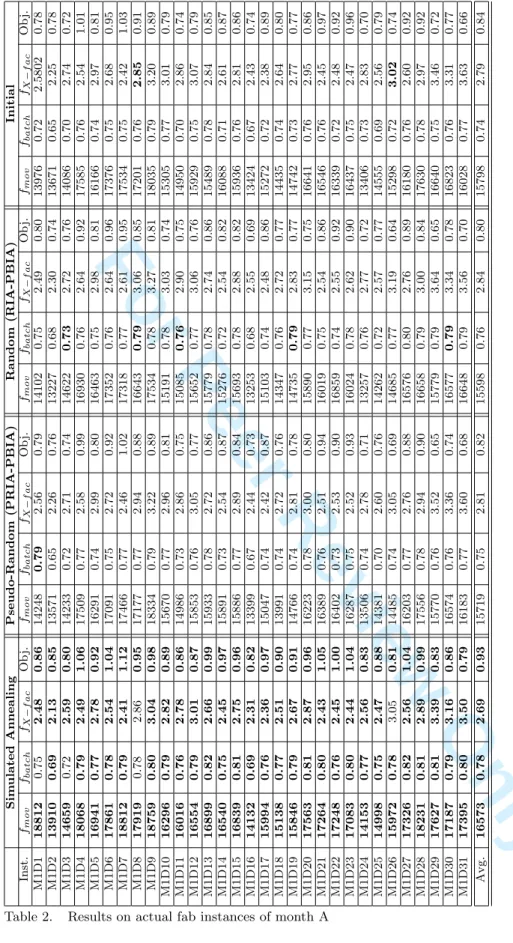
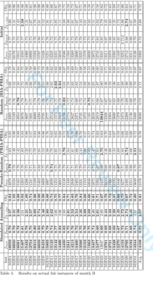
In Tables 2 and 3, we display the objective function solution values (obj), the
num-ber of moves (fmov), the batching coefficient (fbatch) and the X-factor (fX−f ac) obtained
from the three methods: Simulated Annealing (SA), Pseudo (PRIA-PBIA) and Random (RIA-PBIA) algorithms on the basis of solutions obtained by PBIA (Initial). It is im-portant to note that the Simulated Annealing algorithm starts from the best solution of (PRIA-PBIA) and (RIA-PBIA). The best values obtained on each line when comparing
fmov (maximum), fbatch (maximum), fXfac (minimum) and Obj. (maximum) for
Simu-lated Annealing (SA), Pseudo-Random (PRIA-PBIA), Random (RIA-PBIA) and Initial solution (Initial) are also highlighted in bold.
The results obtained with the iterative sampling algorithms PRIA-PBIA (Pseudo-Random) and RIA-PBIA ((Pseudo-Random) are rather disappointing for the two considered months (Months A and B). The indicators are most often worse on average, and are rarely improved when analyzing in details the various instances. This shows that the ranking of the jobs in the initial list used in PBIA is relevant, and helps to provide quite good results. On the other hand, in most of the cases, we are able to substantially improve the initial solution with the simulated annealing algorithm. An improvement of
47.05% on the number of moves fmov is obtained for Month A (resp. 6.6% for Month B),
of 33.04% on the batching coefficient fbatch (resp. 4.15% for Month B), fX−f ac increases
by 41% (resp. by 4.07% for Month B) and the objective function (Obj.) is improved by 11.13% (resp. 12.61% for Month B).
The primary objective of this study was to develop and propose an efficient schedul-ing algorithm to support fabrication operators and improve the main indicators in the diffusion area. The comparison has been done before and after applying our algorithm (PBIA) on the data for the two months. For confidential reasons, we are not allowed to provide the real values of the fab. This is why we give results in percentages on two types of machines. Two indicators are presented: The X-factor and the batching coef-ficient. For the first month, the X-factor on the Type 1 machines is improved by 26% and by 17% for the Type 2 machines. The batching coefficient is also improved by 20% for the Type 1 machines and 29% for the Type 2 machines. For the second month, the X-factor is improved by 36% for the Type 1 machines and 23% for the Type 2 machines. On the other hand, the batching coefficient is deteriorated by 6% for the Type 1 ma-chines and an improvement of 2% is obtained on the Type 2 mama-chines. Our algorithm has been implemented and is currently running. Substantial productivity improvements have been achieved in the diffusion area of the plant thanks to the Priority-based Insertion algorithm (PBIA).
6.2. Experimental tests on data from (M¨onch et al. 2005)
We compare our algorithm (PBIA) to an algorithm proposed in (M¨onch et al. 2005) for
a simplified version of our problem, namely the scheduling problem of jobs on parallel batch processing machines with incompatible job families and unequal ready times. We show through experimental tests that our constructive heuristic PBIA, designed for the specific problem of batching and scheduling in a diffusion area, outperforms the heuristic
described in (M¨onch et al. 2005) on many instances for the problem of minimizing the
Total Weighted Tardiness.
The problem studied in (M¨onch et al. 2005) has the following characteristics:
• Jobs of the same family have the same processing time, • All the batch processing machines are identical in nature,
• Once a machine is started, it cannot be interrupted, i.e. no preemption is allowed.
4 5 6 7 8 9 10 11 12 13 14 15 16 17 18 19 20 21 22 23 24 25 26 27 28 29 30 31 32 33 34 35 36 37 38 39 40 41 42 43 44 45 46 47 48 49 50 51 52 53 54 55 56 57 58 59 60
For Peer Review Only
Sim ulated Annealing Pseudo-Random (PRIA-PBIA) Random (RIA-PBIA) Initial Inst. fmov fbatch fX − f ac Ob j. fmov fbatch fX − f ac Ob j. fmov fbatch fX − f ac Ob j. fmov fbatch fX − f ac Ob j. M1D1 18812 0.75 2.48 0.86 14248 0.79 2.56 0.79 14102 0.75 2.49 0.80 13976 0.72 2.5802 0.78 M1D2 13910 0.69 2.13 0.85 13571 0.65 2.26 0.76 13227 0.68 2.30 0.74 13671 0.65 2.25 0.78 M1D3 14659 0.72 2.59 0.80 14233 0.72 2.71 0.74 14622 0.73 2.72 0.76 14086 0.70 2.74 0.72 M1D4 18068 0.79 2.49 1.06 17509 0.77 2.58 0.99 16930 0.76 2.64 0.92 17585 0.76 2.54 1.01 M1D5 16941 0.77 2.78 0.92 16291 0.74 2.99 0.80 16463 0.75 2.98 0.81 16166 0.74 2.97 0.81 M1D6 17861 0.78 2.54 1.04 17091 0.75 2.72 0.92 17352 0.76 2.64 0.96 17376 0.75 2.68 0.95 M1D7 18812 0.79 2.41 1.12 17466 0.77 2.46 1.02 17318 0.77 2.61 0.95 17534 0.75 2.42 1.03 M1D8 17919 0.78 2.86 0.95 17177 0.77 2.94 0.88 16643 0.79 3.06 0.85 17201 0.76 2.85 0.91 M1D9 18759 0.80 3.04 0.98 18334 0.79 3.22 0.89 17534 0.78 3.27 0.81 18035 0.79 3.20 0.89 M1D10 16296 0.79 2.82 0.89 15670 0.77 2.96 0.81 15191 0.78 3.03 0.74 15305 0.77 3.01 0.79 M1D11 16016 0.76 2.78 0.86 14986 0.73 2.86 0.75 15085 0.76 2.90 0.75 14950 0.70 2.86 0.74 M1D12 16554 0.79 3.01 0.87 15853 0.76 3.05 0.77 15652 0.77 3.06 0.76 15929 0.75 3.07 0.79 M1D13 16899 0.82 2.66 0.99 15933 0.78 2.72 0.86 15779 0.78 2.74 0.86 15489 0.78 2.84 0.85 M1D14 16540 0.75 2.45 0.97 15891 0.73 2.54 0.87 15276 0.72 2.54 0.82 16088 0.71 2.61 0.87 M1D15 16839 0.81 2.75 0.96 15886 0.77 2.89 0.84 15693 0.78 2.88 0.82 15936 0.76 2.81 0.86 M1D16 14132 0.69 2.31 0.82 13399 0.67 2.44 0.73 13253 0.68 2.55 0.69 13424 0.67 2.43 0.74 M1D17 15994 0.76 2.36 0.97 15047 0.74 2.42 0.87 15103 0.74 2.48 0.86 15272 0.72 2.38 0.89 M1D18 15138 0.77 2.51 0.90 13991 0.74 2.72 0.76 14347 0.76 2.72 0.77 14435 0.74 2.64 0.80 M1D19 15846 0.79 2.67 0.91 14766 0.74 2.81 0.78 14735 0.79 2.83 0.77 14742 0.73 2.77 0.77 M1D20 17563 0.81 2.87 0.96 16223 0.78 3.00 0.80 15890 0.77 3.15 0.75 16641 0.76 2.95 0.86 M1D21 17264 0.80 2.43 1.05 16389 0.76 2.51 0.94 16019 0.75 2.54 0.86 16546 0.76 2.45 0.97 M1D22 17248 0.76 2.45 1.00 16402 0.73 2.53 0.90 16859 0.74 2.55 0.92 16339 0.72 2.48 0.92 M1D23 17083 0.80 2.44 1.04 16287 0.75 2.52 0.93 16024 0.78 2.62 0.90 16437 0.75 2.47 0.96 M1D24 14153 0.77 2.56 0.83 13506 0.74 2.78 0.71 13257 0.76 2.77 0.72 13406 0.73 2.83 0.70 M1D25 14998 0.75 2.47 0.88 14381 0.70 2.60 0.76 14262 0.72 2.57 0.77 14555 0.69 2.56 0.79 M1D26 15972 0.78 3.05 0.81 14485 0.74 3.05 0.69 14685 0.77 3.19 0.64 15298 0.72 3.02 0.74 M1D27 17326 0.82 2.56 1.04 16203 0.77 2.76 0.88 16576 0.80 2.76 0.89 16180 0.76 2.60 0.92 M1D28 18231 0.81 2.89 0.99 17556 0.78 2.94 0.90 16658 0.79 3.00 0.84 17630 0.78 2.97 0.92 M1D29 17627 0.81 3.39 0.83 15770 0.76 3.52 0.65 15779 0.79 3.64 0.65 16640 0.75 3.46 0.72 M1D30 17187 0.79 3.16 0.86 16574 0.76 3.36 0.74 16577 0.79 3.34 0.78 16823 0.76 3.31 0.77 M1D31 17395 0.80 3.50 0.79 16183 0.77 3.60 0.68 16648 0.79 3.56 0.70 16028 0.77 3.63 0.66 Avg. 16573 0.78 2.69 0.93 15719 0.75 2.81 0.82 15598 0.76 2.84 0.80 15798 0.74 2.79 0.84Table 2. Results on actual fab instances of month A
To solve this NP-hard problem, the authors propose two different decomposition
ap-1 2 3 4 5 6 7 8 9 10 11 12 13 14 15 16 17 18 19 20 21 22 23 24 25 26 27 28 29 30 31 32 33 34 35 36 37 38 39 40 41 42 43 44 45 46 47 48 49 50 51 52 53 54 55 56 57 58 59 60
For Peer Review Only
Sim ulated Annealing Pseudo-Random (PRIA-PBIA) Random (RIA-PBIA) Initial Inst. fmov fbatch fX − f ac Ob j. fmov fbatch fX − f ac Ob j. fmov fbatch fX − f ac Ob j. fmov fB atch fX − f ac M2D1 16059 0.79 2.57 0.94 14878 0.79 2.63 0.85 14205 0.78 2.68 0.78 15414 0.77 2.60 M2D2 16650 0.79 2.31 1.05 15534 0.76 2.49 0.90 15189 0.76 2.42 0.87 16176 0.75 2.41 M2D3 16081 0.78 2.36 0.98 15165 0.76 2.42 0.89 14954 0.78 2.50 0.84 15015 0.73 2.43 M2D4 15407 0.81 2.61 0.92 14283 0.78 2.63 0.83 13676 0.79 2.72 0.75 14583 0.77 2.58 M2D5 15432 0.78 2.21 1.00 14286 0.75 2.32 0.86 14607 0.77 2.26 0.92 14360 0.73 2.31 M2D6 12754 0.75 2.57 0.74 11241 0.71 2.75 0.57 11601 0.71 2.66 0.58 10992 0.73 2.67 M2D7 16313 0.80 2.60 0.96 15189 0.77 2.78 0.83 14660 0.79 2.78 0.80 15582 0.76 2.76 M2D8 16659 0.83 2.74 0.99 15402 0.82 2.85 0.86 14294 0.79 2.89 0.73 15787 0.80 2.81 M2D9 16453 0.79 2.46 0.99 14809 0.75 2.53 0.86 13795 0.76 2.53 0.76 15428 0.75 2.52 M2D10 15893 0.78 2.80 0.88 14907 0.76 2.88 0.76 13777 0.76 3.00 0.68 15251 0.76 2.91 M2D11 13123 0.74 2.62 0.74 12039 0.74 2.70 0.63 12512 0.73 2.65 0.62 12225 0.72 2.71 M2D12 13142 0.77 2.66 0.75 11253 0.75 2.65 0.65 11573 0.75 2.63 0.62 12451 0.75 2.85 M2D13 14496 0.82 3.06 0.77 13683 0.79 3.15 0.68 12913 0.79 2.84 0.66 13810 0.79 3.11 M2D14 14430 0.82 2.80 0.84 13149 0.79 2.78 0.74 13238 0.82 3.04 0.67 13586 0.78 2.88 M2D15 12341 0.75 2.61 0.71 11349 0.71 2.84 0.57 11774 0.73 2.78 0.59 11504 0.71 2.80 M2D16 14213 0.76 2.53 0.83 12949 0.71 2.61 0.70 12827 0.74 2.63 0.69 13269 0.72 2.61 M2D17 13400 0.72 2.54 0.76 12403 0.70 2.66 0.66 12371 0.69 2.83 0.57 12600 0.70 2.67 M2D18 13566 0.75 2.35 0.84 12231 0.70 2.44 0.70 12725 0.72 2.54 0.68 12255 0.70 2.43 M2D19 12153 0.76 2.80 0.66 11553 0.74 2.98 0.57 11672 0.74 2.92 0.58 11578 0.73 3.01 M2D20 11663 0.75 2.69 0.66 10940 0.73 2.82 0.57 11165 0.75 2.95 0.53 10939 0.73 2.82 M2D21 13457 0.74 2.41 0.81 12872 0.73 2.47 0.74 12650 0.71 2.65 0.66 12672 0.73 2.51 M2D22 13477 0.69 2.61 0.71 13392 0.67 2.83 0.63 12819 0.68 2.87 0.60 12734 0.64 2.82 M2D23 13647 0.69 2.80 0.67 13427 0.66 2.75 0.64 13844 0.67 2.80 0.64 13341 0.65 2.79 M2D24 13761 0.69 2.44 0.76 13234 0.68 2.46 0.70 13328 0.67 2.46 0.71 13211 0.67 2.45 M2D25 12721 0.68 2.33 0.73 12480 0.66 2.60 0.64 12384 0.67 2.59 0.63 12379 0.66 2.63 M2D26 13428 0.69 2.20 0.81 12232 0.65 2.34 0.67 12600 0.65 2.36 0.68 12382 0.65 2.35 M2D27 12270 0.67 2.45 0.68 11846 0.67 2.69 0.59 11379 0.66 2.81 0.51 11449 0.65 2.72 M2D28 14153 0.73 2.72 0.75 13277 0.71 2.84 0.66 13474 0.70 2.89 0.63 13252 0.712 2.86 M2D29 12795 0.71 2.74 0.67 12495 0.68 2.74 0.62 12289 0.69 2.90 0.55 12712 0.68 2.74 M2D30 13182 0.68 2.45 0.72 12314 0.66 2.66 0.60 12136 0.66 2.69 0.57 12311 0.66 2.67 M2D31 14244 0.74 2.57 0.80 13649 0.70 2.51 0.72 13488 0.70 2.70 0.67 13126 0.70 2.59 Avg. 14108 0.75 2.57 0.81 13176 0.73 2.67 0.70 13030 0.73 2.71 0.67 13302 0.72 2.68Table 3. Results on actual fab instances of month B
proaches. The first approach constructs fixed batches, then assigns these batches to the
4 5 6 7 8 9 10 11 12 13 14 15 16 17 18 19 20 21 22 23 24 25 26 27 28 29 30 31 32 33 34 35 36 37 38 39 40 41 42 43 44 45 46 47 48 49 50 51 52 53 54 55 56 57 58 59 60
For Peer Review Only
Average standard deviations Simulated Annealing fmov fbatch fX−f ac Obj
Month A 0.51% 0.62% 0.62% 1.01%
Month B 0.93% 0.50% 1.09% 1.44%
Pseudo-Random (PRIA-PBIA) fmov fbatch fX−f ac Obj
Month A 1.76% 0.58% 1.05% 2.52%
Month B 1.73% 0.60% 0.99% 2.21%
Random (RIA-PBIA) fmov fbatch fX−f ac Obj
Month A 3.93% 1.60% 2.26% 5.76%
Month B 4.21% 1.74% 2.57% 6.33%
Table 4. Average standard deviations for Months A and B
machines using a genetic algorithm (GA) and, finally, sequences batches on each ma-chine. The second approach first assigns jobs to machines using a GA, then constructs the batches on each machine for its assigned jobs and, finally, sequences the batches.
(M¨onch et al. 2005) show in their experiments that the algorithm GA 2 BATC-II, which
belongs to the second type of approach, provides better results on average. We conducted experiments on the (randomly generated) 162 instances with the same computer than the experiments in Section 6.1.
Let us recall that, in this section, the objective function is the Total Weighted Tardiness and that the goal is to compare the Total Weighted Tardiness obtained with our heuristic
(PBIA) to the algorithm GA 2 BATC-II proposed in (M¨onch et al. 2005). Since the input
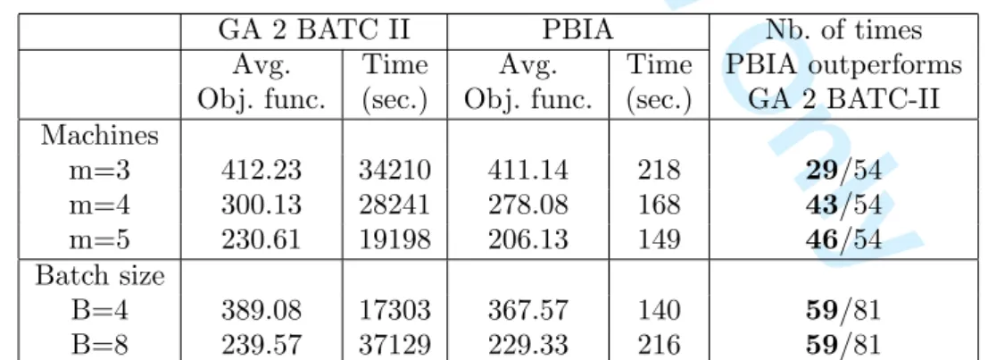
of PBIA is a list and the calculation for one list is fast, we kept the best solution obtained with the two following lists. In the first list, jobs are ordered by increasing order of their due dates and, in the second list, jobs are ordered by decreasing order of their priorities. Starting from the best solution, we apply some local improvements (see Section 5.3). Table 5 shows our results and compares them with the ones obtained with GA 2 BATC-II.
GA 2 BATC II PBIA Nb. of times
Avg. Time Avg. Time PBIA outperforms
Obj. func. (sec.) Obj. func. (sec.) GA 2 BATC-II
Machines m=3 412.23 34210 411.14 218 29/54 m=4 300.13 28241 278.08 168 43/54 m=5 230.61 19198 206.13 149 46/54 Batch size B=4 389.08 17303 367.57 140 59/81 B=8 239.57 37129 229.33 216 59/81
Table 5. Comparison between our proposed algorithm and one of the best algorithms of (M¨onch et al. 2005)
From Table 5, we notice that, on average as well as for the case of m = 3, m = 4 and m = 5, our heuristic (PBIA) performs better in terms of objective function and
1 2 3 4 5 6 7 8 9 10 11 12 13 14 15 16 17 18 19 20 21 22 23 24 25 26 27 28 29 30 31 32 33 34 35 36 37 38 39 40 41 42 43 44 45 46 47 48 49 50 51 52 53 54 55 56 57 58 59 60
For Peer Review Only
computational times. The computational times of our heuristic are more than 100 times smaller than those of GA 2 BATC-II. Among the 162 tested instances, PBIA outperforms GA 2 BATC-II on 118 instances (29 out of 54 for m = 3, 43 out of 54 for m = 4 and 46 out of 54 for m = 5). Furthermore, for a batch size of 4, PBIA outperforms GA 2 BATC-II for 59 instances out of 81 and, for a batch size of 8, also on 59 instances out of 81.
7. Concluding remarks
We proposed a model and methods based on a disjunctive graph representation for a batching and scheduling problem in a semiconductor manufacturing factory while tak-ing into account complex constraints and optimiztak-ing multiple measures. A constructive algorithm has been proposed to solve the problem, local search improvements based on the disjunctive graph representation have been defined and a simulated annealing algo-rithm has been developed. The computational tests made on real instances of the factory showed that good solutions are obtained fast. For the industry, very substantial pro-ductivity improvements have been achieved in the diffusion area and also on the overall fab thanks to the use of the proposed algorithm named Priority rule-Based Insertion algorithm (PBIA).
With adjustments, PBIA has been embedded in a software used by the industry. The use of a disjunctive graph brings significant improvements for interactive scheduling at the fab level. A prototype software includes the off-line batching and scheduling phase, and also an interactive module with a graphical user interface that allows decision-makers to test modifications and validate options on the proposed plan.
The simulated annealing algorithm significantly improves the different criteria (number of moves, batching coefficient and X-factor) in comparison with the initial constructive algorithm. We also compared our approach to an algorithm designed for the problem of scheduling jobs on parallel batch machines with incompatible job families and unequal ready times. The computational tests showed that, for more than half of the instances,
our heuristic outperforms the best algorithm in (M¨onch et al. 2005).
This research can be extended in many ways. Other types of moves such as the simul-taneous move of two jobs linked by a maximum time lag could be tested. The maximum time lags are currently hard constraints. However, in practice, some of them can be re-laxed and treated as soft constraints or objectives. Another important issue would be to perform a more thorough multicriteria analysis. Computing several Pareto optimal solutions may be useful, particularly when the situation frequently changes as it is often the case in semiconductor manufacturing.
Acknowledgments
This work was part of the MEDEA+ European project HYMNE (High Yield driven
MaNufacturing Excellence in sub 65 nm CMOS), partly funded by the “Minist`ere de
l’ ´Economie, de l’Industrie et de l’Emploi” (French Ministry of Economy, Industry and
Employment). 4 5 6 7 8 9 10 11 12 13 14 15 16 17 18 19 20 21 22 23 24 25 26 27 28 29 30 31 32 33 34 35 36 37 38 39 40 41 42 43 44 45 46 47 48 49 50 51 52 53 54 55 56 57 58 59 60
For Peer Review Only
References
Adams, J., Balas, E., and Zawack, D., 1988. The shifting bottleneck procedure for job shop scheduling. Management Science, 34 (3), 391–401.
Balasubramanian, H., et al., 2004. Genetic algorithm based scheduling of parallel batch machines with incompatible job families to minimize total weighted tardiness. In-ternational Journal of Production Research, 48 (8), 1621–1638.
Blazewicz, J., et al., 2007. Handbook on Scheduling: From Theory to Application. Springer.
Cigolini, R., et al., 2002. A new dynamic look-ahead scheduling procedure for batching machines. Journal of scheduling, 5 (2), 185–204.
Dauz`ere-P´er`es, S. and Lasserre, J.B., 1993. A modified shifting bottleneck procedure for
job-shop scheduling. International Journal of Production Research, 31 (4), 923–932.
Dauz`ere-P´er`es, S. and Paulli, J., 1997. An integrated approach for modeling and solving
the general multiprocessor job-shop scheduling problem using tabu search. Annals of Operations Research, 70 (1), 281–306.
Demirkol, E. and Uzsoy, R., 2000. Decomposition methods for reentrant flow shops with sequence dependent setup-times. Journal of Scheduling, 3 (3), 155–177.
Gentner, K., et al., 2004. Batch Production Scheduling in the Process Industries. In: J. Leung, ed. Handbook of Scheduling: Algorithms, Models and Performance Analy-sis. Boca Raton: CRC Press, 481–4821.
Glassey, C. and Resende, M., 1988. Closed-loop job release control for vlsi circuit man-ufacturing. IEEE Transactions on Semiconductor manufacturing, 1 (1), 36–46. Hung, Y., 1998. Scheduling of mask shop E-beam writers. IEEE Transactions of
Semi-conductor Manufacturing, 11 (1), 165–172.
Ibrahim, K., et al., 2003. Efficient Lot Batching System for Furnace Operation. In: Pro-ceedings of IEEE/SEMI Advanced Semiconductor Manufacturing Conference, 322– 324.
Kim, Y., Joo, B., and Choi, S., 2010. Scheduling wafer lots on diffusion machines in a semiconductor wafer fabrication facility. IEEE Transactions of Semiconductor Man-ufacturing, 23 (2), 246–254.
Kirkpatrick, S., Gelatt, C., and Vecchi, M., 1983. Optimization by simulated annealing. Science, tome 220 (4598), 671–680.
Kis, T. and Pesch, E., 2005. A review of exact solution methods for the non-preemptive multiprocessor flowshop problem. European Journal of Operational Research, 164 (3), 592–608.
Kumar, P., 1994. Scheduling semiconductor manufacturing plants. IEEE Control Systems Magazine, 14 (6), 30–40.
Little, J., 1961. A proof for the queuing formula l = λw. Operations Research, 9 (3), 383–387.
Mason, S. and Oey, K., 2003. Scheduling complex job shops using disjunctive graphs: a cycle elimination procedure. International Journal of Production Research, 5 (41), 981–994.
Mason, S., Fowler, J., and Carlyle, W., 2002. A modified shifting bottleneck heuristic for minimizing total weighted tardiness in complex job shops. Journal of Scheduling, 5 (3), 247–262.
Mathirajan, M. and Sivakumar, A.I., 2006a. A Literature Review, Classification and Simple Meta-Analysis on Scheduling of Batch Processors in Semiconductor Man-ufacturing. International Journal of Advanced Manufacturing Technology, 29 (9),
1 2 3 4 5 6 7 8 9 10 11 12 13 14 15 16 17 18 19 20 21 22 23 24 25 26 27 28 29 30 31 32 33 34 35 36 37 38 39 40 41 42 43 44 45 46 47 48 49 50 51 52 53 54 55 56 57 58 59 60
For Peer Review Only
990–1001.
Mathirajan, M. and Sivakumar, A., 2006b. Minimizing total weighted tardiness on het-erogeneous batch processing machines with incompatible job families. International Journal of Advanced Manufacturing Technology, 28 (9-10), 1038–1047.
Mehta, S. and Uzsoy, R., 1998. Minimizing total tardiness on a batch processing machine with incompatible job families. IIE Transactions, 30 (2), 165–178.
M¨onch, L., et al., 2005. Heuristic scheduling of jobs on parallel batch machines with
in-compatible job families and unequal ready times. Computers & Operations Research, 32 (11), 2731–2750.
M¨onch, L., et al., 2009. Scheduling semiconductor manufacturing operations: problems,
solution techniques, and future challenges. In: Proceedings of the Multidisciplinary International Conference on Scheduling : Theory and Applications (MISTA 2009), Aug., Dublin, Ireland, 192–201.
Monch, L. and Habenicht, I., 2003. Simulation-based assessment of batching heuristics in semiconductor manufacturing. In: S. Chick, P. Sanchez, D. Ferrin and D.J. Morrice, eds. Winter Simulation Conference ACM, 1338–1345.
Montoya-Torres, J., 2006. Manufacturing performance evaluation in wafer semiconductor factories. International Journal of Productivity and Performance management, 55 (3-4), 300–310.
Oey, K. and Mason, S., 2001. Scheduling batch processing machines in complex job shops. In: Proceedings of the Winter Simulation Conference, Dec., Arlington, USA, 1200–1207.
Oulamara, A., et al., 2009. FlowShop scheduling problem with batching machine and task compatibilities. Computers & Operations Research, 36 (2), 391–401.
Ovacik, I. and Uzsoy, R., 2007. Decomposition methods for complex factory scheduling problems. Kluwer Academic Publishers.
Perez, I., Fowler, J., and Carlyle, W., 2005. Minimizing total weighted tardiness on a sin-gle batch process machine with incompatible job families. Computers & Operations Research, 32 (2), 327–341.
Pfund, M., et al., 2008. A multi-criteria approach for scheduling semiconductor wafer fabrication facilities. Journal of Scheduling, 11 (1), 29–47.
Su, L., 2003. A hybrid two-stage flow shop with limited waiting time constraints. Com-puters and Industrial Engineering, 44 (3), 409–424.
Sung, C. and Kim, Y., 2003. Minimizing due date related performance measures on two-batch processing machines. European Journal of Operational Research, 147 (3), 644–656.
Sung, C. and Min, J., 2001. Scheduling in a two-machine flowshop with batch process-ing machines for earliness/tardiness measure under a common due date. European Journal of Operational Research, 131 (1), 95–106.
Sze, S., 2001. Semiconductor devices: Physics and technology. John Wiley & Sons, Second Edition.
Uzsoy, R., 1995. Scheduling batch processing machines with incompatible job families. International Journal of Production research, 33 (10), 2685–2708.
Uzsoy, R. and Wang, C., 2000. Performance of decomposition procedures for job-shop scheduling problems with bottleneck machines. International Journal of Production Research, 38 (6), 1271–1286.
Varadarajan, A. and Sarin, S.C., 2006. A survey of dispatching rules for operational control in wafer fabrication. In: Proceedings of 12th IFAC Symposium on Information Control Problems in Manufacturing, 715–726.
4 5 6 7 8 9 10 11 12 13 14 15 16 17 18 19 20 21 22 23 24 25 26 27 28 29 30 31 32 33 34 35 36 37 38 39 40 41 42 43 44 45 46 47 48 49 50 51 52 53 54 55 56 57 58 59 60
For Peer Review Only
Wein, L.M., 1988. Scheduling semiconductor wafer fabrication. IEEE Transactions on Semiconductor Manufacturing, 1 (3), 115–130. 1 2 3 4 5 6 7 8 9 10 11 12 13 14 15 16 17 18 19 20 21 22 23 24 25 26 27 28 29 30 31 32 33 34 35 36 37 38 39 40 41 42 43 44 45 46 47 48 49 50 51 52 53 54 55 56 57 58 59 60