HAL Id: hal-02199848
https://hal-mines-albi.archives-ouvertes.fr/hal-02199848
Submitted on 31 Jul 2019
HAL is a multi-disciplinary open access
archive for the deposit and dissemination of
sci-entific research documents, whether they are
pub-lished or not. The documents may come from
teaching and research institutions in France or
abroad, or from public or private research centers.
L’archive ouverte pluridisciplinaire HAL, est
destinée au dépôt et à la diffusion de documents
scientifiques de niveau recherche, publiés ou non,
émanant des établissements d’enseignement et de
recherche français ou étrangers, des laboratoires
publics ou privés.
Diffracting-grain identification from electron backscatter
diffraction maps during residual stress measurements: a
comparison between the sin 2 ψ and cosα methods
Dorian Delbergue, Damien Texier, Martin Lévesque, Philippe Bocher
To cite this version:
Dorian Delbergue, Damien Texier, Martin Lévesque, Philippe Bocher. Diffracting-grain
identifica-tion from electron backscatter diffracidentifica-tion maps during residual stress measurements: a comparison
between the sin 2 ψ and cosα methods. Journal of Applied Crystallography, International Union of
Crystallography, 2019, 52 (4), pp.828-843. �10.1107/S1600576719008744�. �hal-02199848�
Keywords:X-ray diffraction; residual stress; XRD method comparison; diffracting-grain identification; Debye rings; Inconel 718.
Diffracting-grain identification from electron
backscatter diffraction maps during residual stress
measurements: a comparison between the sin
2w
and cosa methods
Dorian Delbergue,a,bDamien Texier,cMartin Levesqueband Philippe Bochera*
aDepartment of Mechanical Engineering, E´cole de Technologie Supe´rieure, 1100 Rue Notre-Dame Ouest, Qc H3C 1K3,
Montre´al, Canada,bDepartment of Mechanical Engineering, E´cole Polytechnique de Montre´al, Qc H3T 1J4, Montre´al,
Canada, andcInstitut Cle´ment Ader (ICA), Universite´ de Toulouse, CNRS, IMT Mines Albi, INSA, ISAE-SUPAERO, UPS,
Campus Jarlard, F-81013 Albi, France. *Correspondence e-mail: [email protected]
X-ray diffraction (XRD) is a widely used technique to evaluate residual stresses in crystalline materials. Several XRD measurement methods are available. (i)
The sin2 method, a multiple-exposure technique, uses linear detectors to
capture intercepts of the Debye–Scherrer rings, losing the major portion of the diffracting signal. (ii) The cos ! method, thanks to the development of compact 2D detectors allowing the entire Debye–Scherrer ring to be captured in a single exposure, is an alternative method for residual stress measurement. The present article compares the two calculation methods in a new manner, by looking at the possible measurement errors related to each method. To this end, sets of grains in diffraction condition were first identified from electron backscatter diffraction (EBSD) mapping of Inconel 718 samples for each XRD calculation method and its associated detector, as each method provides different sets owing to the detector geometry or to the method specificities (such as tilt-angle number or
Debye–Scherrer ring division). The X-ray elastic constant (XEC)1
2S2, calculated
from EBSD maps for the {311} lattice planes, was determined and compared for the different sets of diffracting grains. It was observed that the 2D detector captures 1.5 times more grains in a single exposure (one tilt angle) than the linear detectors for nine tilt angles. Different XEC mean values were found for the sets of grains from the two XRD techniques/detectors. Grain-size effects were simulated, as well as detector oscillations to overcome them. A bimodal grain-size distribution effect and ‘artificial’ textures introduced by XRD measurement techniques are also discussed.
1. Introduction
Residual stresses play a major role in the fatigue-life behavior of mechanical components (Webster & Ezeilo, 2001; Klotz, Delbergue et al., 2018). Residual stress states resulting from manufacturing or surface treatments are now accounted for in fatigue-life prediction models (Klotz, Miao et al., 2018). Accurate and reliable experimentally measured residual stress profiles are also required for validating predictive models of manufacturing-induced residual stresses (Guagliano, 2001; Frija et al., 2006; Garie´py et al., 2013; Heydari Astaraee et al., 2017; Tu et al., 2017, 2018).
A large number of residual stress measurement techniques exist (Schajer, 2013). The X-ray diffraction (XRD) technique is one of them and has been used for decades, to the extent that some diffractometers are specifically designed for residual stress measurement purposes (Ruud, 2002) and have become
relatively easy to operate. Industry relies intensively on XRD for quality control of fatigue-critical components.
X-rays are electromagnetic radiation whose wavelength is close to crystal lattice spacing. This specific feature can be exploited to measure lattice spacings (Cullity, 1956), d, and a constitutive theory can then be used to compute residual stresses, under the assumption of an elastic crystal lattice distortion (Preve´y, 1986). The technique relies on Bragg’s condition, or the condition for diffraction, defined as
n" ¼ 2d sin #; ð1Þ
where n is a positive integer usually taken as equal to 1, " is the wavelength of the radiation and # is the Bragg angle. The Bragg condition is satisfied when the incident and diffracted X-ray beams are bisected by the normal to the (hkl) diffrac-tion planes. For isotropic polycrystalline materials, the scat-tered X-rays form a cone, called the Debye–Scherrer cone (Howard, 1982). The Debye–Scherrer ring, also named Debye ring, is formed when the diffraction cone intersects a planar detector placed perpendicularly to the incoming X-ray beam (Cullity, 1956; Ho¨rz & Quaide, 1973). A diffraction peak is formed along a given ring radius on the detector. The peak’s relative position on the detector allows determination of the Bragg angle value, and its width can be related to the cold working degree within the irradiated volume (Preve´y, 2000).
Two methods are now mainly used for X-ray residual stress
calculation: the sin2 and the cos ! methods. The
standar-dized sin2 method (SAE International, 2003; ASTM
Inter-national, 2012) is traditionally employed in industry (Fitzpatrick et al., 2005). This method uses part of the Debye ring since the XRD is captured by two linear detectors, such as position-sensitive scintillation detectors, having a fixed posi-tion relative to the incident X-ray beam. Several measure-ments have to be taken at different tilt angles (Noyan & Cohen, 1987), thus sampling different sets of grains. The residual stress associated with the measurements is obtained by linear regression from the slope of the linear relationship existing between the lattice spacings measured at different tilt angles and sin2 values (calculated from the tilt angles).
Technology improvements led to 2D detectors (He, 2009), such as image-plate (IP) detectors (He, 2009; Eatough et al., 1997), facilitating the use of the cos ! method (Taira et al., 1978; Sasaki et al., 1997). The cos ! method relies on the whole Debye ring, which is captured in a single exposure with an IP detector (Hiratsuka et al., 2003) having the incident X-ray beam emanating from its center. The ring’s radius is then used to compute the lattice deformation and the corresponding residual stress value.
The sin2 and cos ! methods rely on different sets of
detected diffracting grains owing to the difference in detector geometry, which may result in different residual stress measurements. Peterson et al. (2017) and others (Sasaki, 2014; Delbergue et al., 2016; Kohri et al., 2016; Ramirez-Rico et al., 2016; Delbergue et al., 2017) have reported differences in results when measuring residual stresses with the two methods. However, Peterson et al. (2017) were able to reduce the differences between the two methods in shot-peened
standard-sample residual stress measurements with the generalized least-squares analysis proposed by Miyazaki & Sasaki (2016). Miyazaki & Sasaki (2016) have shown, on the basis of the fundamental equations, that the only differences between the sin2 and cos ! methods lie in the fact that the sets of diffracting grains are different for these two methods and the crystalline grain aggregates exhibit local elastic property variations (Kocks et al., 1998).
Authors who compared the residual stress measurements
resulting from the sin2 and cos ! methods have mostly
focused on experimental observations (Delbergue et al., 2016; Kohri et al., 2016; Ramirez-Rico et al., 2016; Peterson et al., 2017) or on the fundamental equations (Ramirez-Rico et al., 2016; Miyazaki & Sasaki, 2016), but none have numerically compared the two methods using the coupling between the stress calculation method and the inhomogeneous grain response to elastic deformation. By relying on crystal plasti-city, Erinosho et al. (2016) have simulated lattice strains by considering grains that satisfy the diffraction condition and compared their predictions against in situ synchrotron XRD measurements.
The principal objective of this article is to compare the sin2 and cos ! methods in terms of diffracting-grain number and X-ray elastic constant (XEC) of the diffracting-grain set, according to the detector specificities. The comparison was made by identifying the diffracting grains for the two methods from electron backscatter diffraction (EBSD) grain orienta-tion maps and evaluating their average elastic properties. To the best of our knowledge, the comparison of the two methods has never been done using the XEC estimated for sets of diffracting grains from EBSD maps. The article is organized as
follows: The fundamental equations for the sin2 and cos !
methods are presented in Section 2. In Section 3, the studied material, its microstructure, the two XRD measurement conditions, the grain conditions for diffraction and the XEC calculation method are presented. Experimental and numer-ical results such as EBSD maps, identified diffracting grains, calculated XEC and ‘artificial’ textures of the XRD measurement methods are set out in Section 4. The results are then discussed in Section 5 before the conclusion of this work.
2. Residual stress measurement theory
For crystalline or polycrystalline materials, the measurement of residual stresses using X-ray diffraction techniques is based on the change of lattice spacing, d, and each grain is basically used as a local strain gauge. For instance, the presence of tensile residual stresses within the irradiated volume increases the d spacing in a given direction, resulting in a diffraction peak shift towards lower # values. The shift yields a Bragg angle value, #, which differs from the #0value obtained for a
stress-free sample of the same material (usually measured on powder).
In XRD measurements, the strain, "fhklg’ , is measured along
the diffraction vector Vhkl defined in the sample coordinate
Vhkl¼ v1 v2 v3 0 @ 1
A ¼ sin cos ’sin sin ’ cos 0 @
1
A; ð2Þ
where ’ and are the azimuthal and tilt angles, respectively (the angles are defined in Fig. 1). The measured strain, "fhklg’ , can be computed from the measured Bragg angle, #, or the planes’ lattice spacing, dfhklg’ , and can be obtained by
"fhklg ’ ¼
dfhklg’ $ dfhklg0
dfhklg0
¼ $!# cot #0; ð3Þ
where !# = #$ #0and d0is the d spacing corresponding to the
#0 value, measured for a stress-free sample. The strain
measured along the diffraction vector Vhkl can then be
expressed in terms of the strain components "ij in sample
coordinates with respect to the Einstein summation conven-tion by "fhklg ’ ¼ dfhklg’ $ dfhklg0 dfhklg0 ¼ vivj"ij; ð4Þ
where viand vjare the Vhkl components defined in equation
(2). If the measured material is isotropic and homogeneous, Hooke’s law can be used to relate the macroscopic stress, $, to the strain as "ij¼ 1þ % E $ij$ &ij % E$kk; ð5Þ
where E and % are the material’s macroscopic Young modulus and Poisson ratio values, respectively, and & is the Kronecker delta. Assuming that the material is macroscopically not textured and composed of fine grains, and if the stress in the irradiated layer is assumed to be biaxial (i.e. $33= $23= $13=
0), the measured strain can be related to the macroscopic stress through "fhklg’ ¼d fhklg ’ $ dfhklg0 dfhklg0 ¼ 1þ %fhklg Efhklg $’sin 2 $%fhklg Efhklgð$11þ $22Þ; ð6Þ where E{hkl}and %{hkl}are the equivalent Young modulus and
Poisson ratio determined for the {hkl} planes, respectively. $’¼ $11cos2’ þ $12sin 2’þ $22sin2’ is the macroscopic
stress along the direction ’ defined by the linear detector plane (see Fig. 1). The use of E{hkl}and %{hkl}allows the crystal
anisotropy to be taken into consideration to relate the strain measured on crystallographic planes to the macroscopic stress.
We define Sfhklg1 and12S fhklg
2 as the XECs for the {hkl} planes
as Sfhklg1 ¼$% fhklg Efhklg ; ð7aÞ 1 2Sfhklg2 ¼ 1þ %fhklg Efhklg : ð7bÞ
The stress $’can be obtained by differentiating equation (6)
with respect to sin2 as
$’¼ Efhklg 1þ %fhklg @"fhklg ’ @ sin2 ¼ 1 1 2Sfhklg2 @"fhklg ’ @ sin2 ; ð8Þ
which shows that only1
2Sfhklg2 has to be known to determine $’.
When plotting the measured strain "fhklg’ as a function of sin2 , and on the basis of the assumptions listed previously, one can determine the stress $’, in the measurement direction ’, if a
linear regression between "fhklg’ and sin2 is performed.
Therefore, several angles have to be used to obtain the relationship between "fhklg’ and sin2 when the diffracted
X-rays are captured with two linear detectors. In practice, the
several angles needed, which correspond to different Vhkl
vectors, are obtained when changing the incident X-ray beam angle, ' = & ( (2( = ) $ 2# being the diffraction cone semi-apex angle shown in Fig. 1).
The stress calculation can be done with a single X-ray exposure when the whole Debye ring is measured. For a stress-free material, such as a powder, the Debye ring is perfectly circular, as the lattice spacings, dfhklg0 , are the same in
every direction. A stressed surface will modify the ring radius and its distortion can be described using the ! angle defined as the polar angle along the Debye ring, as schematized in Fig. 1.
The strain is measured along Vhkl for different ! angles.
Therefore, when the measurement is made with a planar detector, the diffraction vector Vhklshould be defined in the
sample coordinate system using the angle ! and the diffraction cone’s semi-apex angle 2( as
Vhkl¼
cos ( sin ' cos ’$ sin ( cos ' cos ’ cos ! $ sin ( sin ’ sin ! cos ( sin ' sin ’$ sin ( cos ' sin ’ cos ! þ sin ( cos ’ sin !
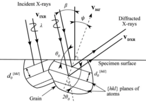
cos ( cos 'þ sin ( sin ' cos ! 0 B @ 1 C A: ð9Þ Figure 1
Schematic representation of a sample, the diffraction cone resulting from the diffraction of {hkl} planes, and the measurement planes related to the linear and 2D detectors (sin2 and cos ! methods, respectively). List of
the symbols: d{hkl}: lattice spacing of the {hkl} planes; V
hkl: diffraction
vector; S: sample coordinate system; 2#: Bragg angle; 2(: diffraction cone semi-apex; ': incident X-ray beam angle; : angle between the {hkl} plane normal and sample normal (tilt angle); ’: azimuthal angle;r’: residual
stress measurement direction; !: 2D detector angle; R!: Debye ring radius
For a given !-angle position on the 2D detector, the measured strain "fhklg
! can be obtained from the ring radius R!as
"fhklg
! ¼ $!# cot #0¼12 2#0$ ) þ tan$1ðR!=CLÞ
! "
cot #0;
ð10Þ
where CL is the sample-to-detector distance. Similarly to
equation (4), the measured strain "fhklg
! can be related to the
strain components "ijin sample coordinates with respect to the
Einstein summation convention as "fhklg
! ¼ vivj"ij: ð11Þ
We define the parameter "fhklg! as
"fhklg
! ¼12 ð"fhklg! $ "fhklg)þ!Þ þ ð"fhklg$! $ "fhklg)$!Þ
! "
; ð12Þ
where "fhklg
! , "fhklg)þ!, "fhklg$! and "fhklg)$!are strains determined at four
points located at 90' on the Debye ring for a given ! angle
varying from 0 to 90'using equation (10). The cos ! method
yields the stress $’thanks to some trigonometric
simplifica-tions. When a biaxial stress state is assumed in the irradiated layer and if the material’s microstructure is composed of fine grains with a macroscopically isotropic elastic behavior, the parameter "fhklg! can be expressed in terms of stresses by
combining equations (5), (11), (9) and (12) as "fhklg
! ¼ $
1þ %fhklg
Efhklg sin 2( sin 2' cos ! $’; ð13Þ
where $’= 1=2½$11ð1 þ cos 2’Þ þ $22ð1 $ cos 2’Þ þ 2$12sin 2’).
Differentiating equation (13) with respect to cos ! and isolating $’yields $’¼ $ Efhklg 1þ vfhklg 1 sin 2( sin 2' @ "fhklg ! @ cos ! ¼ $1 1 2Sfhklg2 1 sin 2( sin 2' @ "fhklg ! @ cos !: ð14Þ
The stress $’ can be obtained when plotting the parameter
"fhklg
! as a function of cos ! and if a linear regression between
"fhklg
! and cos ! is performed.
3. Material and experimental procedures
3.1. Material
This study focused on the nickel-base superalloy Inconel 718 (IN718), which was subjected to a solution and precipi-tation heat treatment as per AMS 5663M (SAE International, 2009). The material’s chemical composition and macro-tensile properties were determined in previous work (Klotz, Delbergue et al., 2018) and are listed in Tables 1 and 2, respectively. Two samples extracted in the rolling direction of bars with initial diameters of 25.4 mm (1 in) and 76.2 mm (3.5 in) were investigated. As they provide different micro-structure, the bars’ initial diameters in inches will be used to refer to the samples. The sample surfaces were carefully prepared by grinding using SiC papers (down to grade 1200/
P4000), and a layer of 5mm was then removed by
electro-polishing to obtain surfaces that were almost free of residual stress and work hardening.
The nickel-base superalloy being a face-centered cubic (f.c.c.) polycrystalline material, the {311} family of atom planes is used since they diffract for high 2# Bragg angles, reducing the sensitivity of the strain to the precision of the Bragg angle measurement. In this condition, 24 planes of symmetry are available, meaning that 24 planes can possibly contribute to the diffraction of X-rays.
3.2. Diffractometers for XRD measurements
We consider two dedicated diffractometers, one for each stress calculation method, that could be used for residual stress measurements. A Proto iXRD apparatus equipped with two linear detectors (position-sensitive scintillation detectors)
and an Mn tube could be used to investigate the sin2
method, and a Pulstecm-X360n apparatus equipped with a 2D
detector (IP detector) and a Cr tube could be used when capturing the whole Debye ring for the cos ! method. The Proto iXRD Mn tube allows measurement of the deformation of the IN718 {311} planes from filtered K! lines, whereas use
of the Pulstecm-X360n Cr tube implies measuring it from the
K' line. The K! and K' lines are explained in standard reference books (Cullity, 1956; Noyan & Cohen, 1987). Typical diffraction conditions for IN718 and for both apparatuses are listed in Table 3.
3.3. Microstructural characterization method
EBSD scans were performed to characterize the grain-size distribution, quantify the degree of crystallographic texture and investigate the effect of the set of grains participating in
Table 1
Inconel 718 chemical composition obtained by optical spectrometry (wt%).
Elements Ni Fe Cr Nb Mo Ti Al Co Mn Si
Composition Balance 19.53 17.84 5.02 3.07 1.16 0.64 0.35 0.16 0.06 Table 2
Inconel 718 macrotensile properties.
E: Young’s modulus; $y0.2%: 0.2% offset yield strength; $u: ultimate strength; El.: elongation at failure.
E (GPa) $y0.2%(MPa) $u(MPa) El. (%)
Table 3
Typical X-ray diffraction conditions for Proto iXRD (sin2 method) and
Pulstecm-X360n (cos ! method) apparatuses.
Proto iXRD
Pulstec m-X360n
Tube (X-ray lines) Mn K! Cr K'
Wavelength (A˚ ) 2.291 2.085
Bragg angle 2#0(') 151.8 148.2
Diffraction planes/dfhklg0 {311}/df311g0 = 1.08 A˚
Collimator (mm) 1 1
Voltage (kV)/current (mA) 23/2.5 30/1.0
Total measurement time (min) 8 1.5
No. of inclinations 9 1
' inclinations (') [&25 &19.01 &14.06 &7.27 0] 30
the XRD measurements on the XEC values. The scans were carried out on areas having sizes similar to the irradiated areas
during XRD measurements (*2 mm2). A conventional
Hitachi SU-70 scanning electron microscope equipped with a Bruker camera and HKL Channel 5 software from Oxford Instruments were used for the EBSD scans. Table 4 summarizes the subset and total map areas measured with a step size of 0.5mm.
Grain-size distributions and the crystallographic texture were determined by post-treatment using MATLAB (The MathWorks Inc., Natick, MA, USA) and the MTEX open-source package (Bachmann et al., 2011). Grains were identi-fied using a grain-detection angle of 10'. Twins were
consid-ered as unique grains to limit the artifacts arising from the determination of the grain’s mean orientation, thus increasing the total number of indexed grains. The orientation distribu-tion funcdistribu-tions (ODFs) were calculated using the de la Valle´e Poussin kernel (Hielscher, 2013) and all measurement points to account for grain-size effects from surface observation. Sample texture analyses are presented as inverse pole figure plots with respect to the rolling direction. Texture analyses associated with XRD measurements are also presented using pole figures.
3.4. Identification of diffracting grains
A MATLAB script using the MTEX open-source package has been developed to identify the grains meeting the Bragg condition for the two types of detector. Under this condition and for an unstressed sample, the diffracting planes have to
make an angle #0 with the incoming X-rays to scatter the
incoming X-ray beam for the particular planes under consid-eration, i.e. {311}, as shown in Fig. 2. In this figure, VIXR, VDXR
and Vhklare unit vectors representing the incident X-rays, the
diffracted X-rays and the vector normal to the {hkl} planes, respectively. To meet the conditions of Bragg’s law, Vhklhas to
be the bisector vector of VIXR and VDXR, providing a
geometrical condition for selecting the diffracting grains. The MTEX package was used for calculating each grain’s mean orientation. The Vhklvector can thus be determined for any (h,
k, l) Miller indices and the condition for diffraction can be expressed by the dot product of VIXRand Vhkl. Each grain can
be associated with an angle #xdefined as
#x¼ cos$1
VIXR+ Vhkl
kVIXRkkVhklk
# $
; ð15Þ
and diffraction can take place when #x= (90$ #0). A tolerance
of 2'was used to replicate the XRD line-broadening effect,
allowing some deviation from the exact Bragg condition. The
2' tolerance is close to half the diffraction-peak widths
experimentally obtained for both techniques in previous work (Delbergue et al., 2017; Klotz, Delbergue et al., 2018), focusing the investigation on the diffraction information coming from the highest intensities of potential diffraction peaks.
3.5. XEC calculation
The XEC1
2S fhklg
2 of the diffracting grains was determined for
comparison purposes using the MTEX package (Mainprice et al., 2011) as follows:
(i) An IN718 single-crystal stiffness tensor, CIN718, was
assigned to all the grains of the EBSD map: C11= 251.0 GPa,
C12 = 135.5 GPa and C44= 98.0 GPa. The coefficients have
been chosen from among the experimental values reported in the literature (Ledbetter & Reed, 1973; Margetan et al., 2005; Haldipur, 2006; Aba-Perea et al., 2016) at room temperature for a certain range of grain sizes and compositions.
(ii) An ODF, f, was calculated for the set of diffracting grains to account for the possibility of some anisotropy introduced by the XRD measurement.
(iii) The ODF was then used to determine the average stiffness tensor of the set of diffracting grains computed for the Voigt and Reuss bounds (assuming a constant elastic strain and stress, respectively, in all crystallites) as (Mainprice et al., 2011) hCiSVoigt ¼ P M m¼1 CIN718ðgmÞ !mfðgmÞ; ð16aÞ hCiSReuss ¼ P M m¼1 C$1IN718ðgmÞ !mfðgmÞ % &$1 ; ð16bÞ
wherehCiSVoigt
andhCiSReuss
are the average stiffness tensors expressed in the sample reference system, S, for the Voigt and Reuss bounds, respectively, and are calculated for the selected
set of m diffracting grains having an orientation gm and a
weight !m. The angle brackets denote the average over the
grains that satisfy a particular diffraction condition.
(iv) The XEC1
2S fhklg
2 was calculated with the quasi-isotropic
XEC equation used in the case of biaxial stress state (Van Houtte & De Buyser, 1993):
Table 4
EBSD subset map size and total map area for 1 and 3.5 in samples.
Sample Subset map size (mm) Total map area (mm2)
1 in 317, 237.5 1.414
3.5 in 635, 476 1.154
Figure 2
Illustration of X-rays diffracted by {hkl} planes of an unstressed grain in the Bragg condition. In this condition, the diffraction vector Vhklbisects
the incident X-rays VIXRand the diffracted X-rays VDXR, such that they
make an angle #0with the {hkl} planes having a lattice spacing dfhklg0 . List
of symbols: ': incident X-ray beam angle; : angle between the {hkl} plane normal and sample normal (tilt angle); ": X-ray wavelength.
1
2Sfhklg2 ¼ hS3333iL$ hS3311iL; ð17Þ
where hS3333iL and hS3311iL are the
fourth-rank compliance tensor coefficients of
hSijkliL¼ aimajnakoalphSmnopiSexpressed in the
laboratory system, L, with
hSijkliS¼ ðhCijkliSÞ$1. The laboratory system is
defined as having the z axis coincident with the diffraction vector, and aij is the rotation
matrix from the S system to the L system.
1
2Sfhklg2 was computed for the Voigt and Reuss
bounds.
(v) Finally, as the experimentally measured elastic constants are often close to the average of the Voigt and Reuss bounds (Hill,
1952; Gna¨upel-Herold et al., 1998; Murray, 2013), the Neer-feld–Hill limit, which is the arithmetic mean of the Voigt and Reuss bounds, was used during the study:
1 2Sfhklg2 ' (Hill ¼1 2 12Sfhklg2 ' (Voigt þ 1 2Sfhklg2 ' (Reuss h i : ð18Þ
Note that the hhkli crystallographic direction is taken into
consideration in the calculation of f(gm) as it is computed for
the identified diffracting grains. When computed for the {311} planes, the XECð1
2S f311g 2 Þ
Hill
is denoted in this article as1 2S
f311g 2
for convenience.
This procedure for the1
2S f311g
2 computation was carried out
for each of the different ' tilts and linear detectors for the
sin2 method and for each combination of ' tilt and !-angle
position for the cos ! method. 4. Results
4.1. Microstructure analyses
The grain microstructure was characterized by EBSD over regions representative of the X-ray irradiated zones. Large areas in the RD–TD plane were scanned for both 1 and 3.5 in samples. The resulting maps were plotted for the RD using inverse pole figures (IPFs) and are presented in Fig. 3 (RD: rolling direction; TD: transverse direction; ND: normal direction). Each color corresponds to a crystal orientation. The 1 in sample has a fine and homogeneous grain-size distribution, while the 3.5 in sample exhibits a bimodal microstructure composed of small grains and a few large grains. The grains’ equivalent diameter distributions are presented as a function of the area they occupy in Fig. 4. A 6mm average grain size was calculated for the 35 805 detected grains for the 1 in sample, whereas the average grain size was
8mm for the 3.5 in sample and 10 610 grains were detected
[corresponding to an ASTM grain-size number of 12 and 11
(ASTM International, 2013), respectively]. Table 5
summarizes the grain distribution for the two specimens. The 3.5 in sample’s bimodal microstructure is documented in Fig. 4(b) (inset), where the grains are divided into two families: the ‘large grains’ were defined as the grains larger than the average grain size plus four times the equivalent diameter standard deviation (SD), i.e. an equivalent diameter
higher than 42mm [the equivalent diameter, ;, is calculated as ; = 2(A/))1/2, where A is the grain area]. Ninety-three large
grains (0.87% of the grain population) were found, occupying 26% of the map area.
The crystallographic textures are presented in Fig. 5 as IPF plots with respect to the RD, for both samples. No preferred
Figure 3
Orientation distribution maps for the 1 and 3.5 in samples, represented as inverse pole figure maps with respect to the rolling direction.
Figure 4
Grain-size distribution in percent of area ratio for (a) the 1 in sample and (b) the 3.5 in sample. The equivalent diameter,;, is calculated as ; = 2(A/ ))1/2, where A is the grain area. In the inset, ‘large grains’ describes the
grains having a diameter of at least the average diameter plus four times the diameter standard deviation (; > 42 mm).
orientation is observed for the 1 in sample with a texture index of 1.15, whereas for the 3.5 in sample, a slightly higher occurrence of theh001i crystallographic orientations is found in the RD, but with a low index of around 1.9. Such a texture is often observed after recrystallization of a rolled f.c.c. material (Etter & Baudin, 2013). Nevertheless, neither sample can be considered as highly textured. The crystallographic directions of interesth311i are also shown in Fig. 5.
4.2. Diffracting grains
4.2.1. Identification of the diffracting grains. The grains in the diffraction condition were first identified using the devel-oped MATLAB script on the 1 in sample, as it represents the
ideal case of a homogeneous microstructure. The XRD conditions and diffractometer parameters used in the script are listed in Table 3. The maximum effective penetration depth, when computed for the two radiations and detector types, as described in the work of Noyan & Cohen (1987) and Tanaka (2018) for the sin2 and cos ! methods, respectively,
was found to be 5mm, which is less than the smaller average
grain size (6mm). Therefore, it is assumed that only the layer of grains obtained by EBSD could diffract.
Figs. 6(a) and 6(b) present in IPF coloring the diffracting grains if X-ray diffraction was captured by the two linear detectors of the Proto iXRD and the 2D detector of the Pulstecm-X360n, respectively. Fig. 6(a) is the superimposition of the diffracting grains captured by the two linear detectors for nine acquisition positions (the nine ' angles listed in Table 3). Fig. 6(b) shows the diffracting grains seen by the 2D
detector for a single exposure at ' = 30'. The number of
diffracting grains was calculated in the two situations and is reported in Table 6. The grains contributing to the diffraction data represent 15.0 and 22.4% of the EBSD map area for the
sin2 and cos ! methods, respectively. The 2D detector thus
samples 32% more unique diffracting grains than the linear detectors swept along nine ' angles. Only 1129 unique grains are identified both by the two linear detectors (5540 identified diffracting grains) and by the 2D detector (8183 identified diffracting grains), corresponding to 20 and 14%, respectively. Some of these shared diffracting grains can be observed in Fig. 6.
4.2.2. Simulation of detector windows. The intersections of the diffraction cone with the linear and 2D detectors were simulated, to
better understand how the 2D
detector can see 32% more diffracting grains in a single exposure than the two linear detectors in nine exposures. Figs. 7(a) and 7(b) present the simu-lated images seen by the two linear
detectors at ' = 25' and by the 2D
detector at ' = 30', respectively, for a
single exposure. Each circular symbol represents the localization of X-rays scattered by a diffracting grain inter-secting the detector plane (as illu-strated in Fig. 1). The diffracting
grains’ mean orientations are
presented using IPF coloring with respect to the RD. The X axis is parallel to the RD while the Y axis is
Table 6
Number of grains contributing to the XRD when data are captured by two linear detectors or a 2D detector for the 1 in sample.
Proto iXRD Pulstecm-X360n
Detector type Linear detectors 2D detector
No. of diffracting grains 5540 8183
Grain percentage (%) 15.5 22.9
Area percentage (%) 15.0 22.4
Table 5
Grain size and grain density for 1 and 3.5 in samples.
Grain equivalent diameter (mm)
Sample Mean SD Minimum Maximum Grain density (grains mm$2)
1 in 6 4 1 31 25316
3.5 in 8 8 1 140 9200
Figure 6
Orientation distribution maps of the 1 in sample presenting the diffracting grains detected by (a) the two linear detectors for nine inclinations (Proto iXRD) and (b) the 2D detector for a single exposure (Pulstecm-X360n). The IPF representation with respect to the RD has been kept.
Figure 5
Inverse pole figures for the texture analysis of the (a) 1 in and (b) 3.5 in samples with respect to the rolling direction. Theh311i directions are also shown.
parallel to the TD, and the incoming X-rays (not represented here) would be at the coordinates (0, 0). The two linear detectors can be observed in Fig. 7(a) with the presence of two distinct regions. The full Debye ring is captured by the 2D detector as shown in Fig. 7(b). Note that the Y width of the regions in Fig. 7(a) is related to the width of the linear
detectors, whereas the X width is linked to the 2' tolerance
angle used for the identification of the diffracting grains, which also corresponds to the ring width in Fig. 7(b).
4.3. Angle variations
4.3.1. Linear detectors: number of used b angles. Three to 21 ' angles have been simulated for the same range of
maximum angles: &25'. Increasing the number of ' angles
would increase not only the number of diffracting grains but also the measurement time. Fig. 8 presents the number of unique diffracting grains versus the number of ' angles. The values are compared with the number of unique diffracting
grains seen by the 2D detector for a measurement at ' = 30'
[the grains highlighted in Fig. 6(b)]. The case of nine ' angles corresponds to the number of measurements at which the
number of additional diffracting grains starts to decrease with increasing number of ' angles.
The total number of diffracting grains stays below the 8183 unique grains contributing to the diffraction captured by the 2D detector, even for a high number of linear-detector posi-tions (e.g. 21 ' angles). Increasing the number of ' angles further than 21 does not increase the number of unique diffracting grains owing to the superimposition of the ' positions.
4.3.2. 2D detector: effect of b angle. The influence of the X-ray incident angle on the number of diffracting grains has been studied for the cos ! method. ' angles ranging from 10 to 45'have been simulated. Fig. 9 presents the number of unique
diffracting grains for the different 2D detector inclinations. The figure shows that the number of unique diffracting grains remains almost constant, regardless of the ' angle. This observation might result from the fact that the 1 in sample exhibits an isotropic distribution of the grains’ mean orienta-tions.
4.3.3. 2D detector: variation along the a values. The parameter "fhklg! is computed, for a given ! angle, from the
strains measured at four orthogonal positions on the Debye
Figure 7
Simulated images seen by (a) the two linear detectors (' = 25') and (b)
the 2D detector (' = 30') for the 1 in sample. Diffracting grains are
represented by circular symbols, and IPF coloring with respect to the RD
is used to show their mean orientations. Figure 9
Total number of unique diffracting grains seen by the 2D detector versus the detector ' angle.
Figure 8
Total number of unique diffracting grains versus the number of ' angles taken by the two linear detectors in a&25'range. The number of unique
diffracting grains contributing to the 2D detector data for a single exposure at ' = 30'is plotted as a dash–dot line for comparison.
Figure 10
Simulated Debye ring on the 2D detector for ' = 30'. Each circle
represents a diffracting grain. The diffracting grains used for the calculation of "fhklg
ring. Consequently, the full scan of the Debye ring is carried out for a varia-tion of ! from 0 to 90'. Therefore, only
a small part of the collected data is used for computing the strain for a given !. Fig. 10 presents a simulated Debye ring seen on a 2D detector for a single exposure at ' = 30'. Each circle
corresponds to a given diffracting grain. The grains used for the calcula-tion of "fhklg! at ! = 45.36' are
high-lighted in red as an example. The !-step size being set to 0.72', 125 ! angles
are used to compute the 125 "fhklg!
values. The "fhklg! values may then be
plotted versus the corresponding cos ! values to determine the residual stress. In the case where no diffracting grains are detected for a given !, the !-step size could be increased to allow "fhklg!
values to be computed.
4.4. XRD texture measurement
Different sets of diffracting grains are detected when using the two diffraction techniques, and different
crystallographic textures may be obtained via the linear detec-tors and the 2D detector during XRD measurements. Using the developed script and the MTEX package, pole figures can be plotted for the homogeneous microstructure of the 1 in bar, showing the diffracting grains for the two different types of detectors. The pole figures for the (100), (110), (111) and (311) sets of planes are presented in Figs. 11(a), 11(b) and 11(c) for all the grains of the 1 in sample, and only for the diffracting grains detected by the two linear detectors and the 2D detector, respectively. The (311) pole figure has been plotted in addition to the traditional (100), (110) and (111) pole figures to present the textures introduced by XRD measure-ments of the planes used for strain measuremeasure-ments.
Like Fig. 6(a), Fig. 11(b) is the superimposition of the different positions taken by the linear detectors. However, Figs. 12(a), 12(b) and 12(c) show the pole figures for three specific ' angles taken by the linear detectors: ' =$25', ' = 0'
and ' = 25', respectively. For each pole figure, two hot spots
representing the localization of the two linear detectors can be observed. They are the centers of concentric circles. The detector motion during the residual stress measurements can be observed as a straight line at the center of the (311) pole figure in Fig. 11(b), which results from the displacement of the concentric circles, illustrated in Fig. 12. On the other hand, the 2D detector, by its geometry, allows the Debye ring to be captured in its entirety, which results in the circle of high index visible in the (311) pole figure of Fig. 11(c). The concentric circles are not centered because of the incident angle of the
X-ray beam (' = 30'). Nonetheless, the cos ! method implies
dividing the Debye ring for the "fhklg! calculation, as shown in
Fig. 10, which results in the intermediate textures presented in Fig. 13. The ! steps providing the highest and the lowest texture indexes are presented in Figs. 13(a) and 13(b),
Figure 12
Pole figures of the (311) diffracting planes for the two linear detectors at (a) ' =$25', (b) ' = 0'and (c) ' = 25'.
Figure 13
Pole figures of the (311) diffracting planes for the 2D detector for the ! angles providing the maximum and minimum texture indexes at (a) ! = 0.72'and (b) ! = 25.2', respectively, as well as the ! = 45.36'example.
Figure 11
Pole figures of the (100), (110), (111) and (311) sets of planes for (a) the whole 1 in sample EBSD map and for the diffracting grains detected by (b) the linear detectors and (c) the 2D detector. Note that the (311) set of planes is the strain measurement set of planes used for residual stress computation.
respectively. Fig. 13(c) corresponds to the pole figure of the highlighted grains given as an example in Fig. 10. The four
strain measurements at !, ) + !,$! and ) $ ! imply four hot
spots [visible in Figs. 13(b) and 13(c)], the centers of four concentric circles, but because of the low !-step size the circles are not clearly defined. Furthermore, for ! values close to 0'
or to 90', only two hot spots can be distinguished, which
results in higher maximum texture indexes.
Fig. 11(a) confirms that the 1 in sample is not textured with a maximum index of 1.65, while the pole figures of the diffracting grains detected by the two types of detectors [Figs. 11(b), 11(c), 12 and 13] exhibit two different types of textures. These textures are related to the type of detector used for XRD measurements. This ‘artificial’ texture may affect the XEC value of the diffracting grains and therefore the measured stress, as the stress is linearly dependent on the XEC value in both calculation methods.
4.5. XEC values for the diffracting grains
The average XEC 1
2S fhklg
2 was determined for the {311}
planes of the diffracting grains in terms of the Hill limit. As described in Section 3.5, ODFs were used for XEC calcula-tions to take into account the ‘artificial’ texture created by XRD conditions.
The1
2Sfhklg2 Voigt and Reuss bounds can be computed as a
reference for the case of an isotropic polycrystal and for the stiffness tensor given in Section 3.5 as (Van Houtte & De Buyser, 1993) 1 2S fhklg 2 ' (Voigt ¼ 10S1212ðS1111$ S1122Þ 3S1111$ 3S1122þ 4S1212 ; ð19aÞ 1 2Sfhklg2 ' (Reuss ¼ S1111$ S1122$ 3S0"; ð19bÞ
where S1111, S1212and S1122are the coefficients of the
single-crystal compliance tensor [SIN718¼ ðCIN718Þ$1], S0 = S1111 $
S1122$ 2S1212, and " is the orientation parameter defined as
"¼h
2k2þ h2l2þ k2l2
ðh2þ k2þ l2Þ2 : ð20Þ
Only the Reuss bound is hkl dependent. When computed for the case of the {311} planes, the Voigt and Reuss bounds are 6.11, 10$6and 6.98, 10$6MPa$1, respectively. Finally, the
Hill limit computed using equation (18) is 6.54, 10$6MPa$1.
Fig. 14 presents the XEC values for the nine ' angles used for residual stress measurements using the linear detectors as well as the number of diffracting grains detected for each position. The results are separately given for the two linear detectors, namely the left and right detectors [they correspond in Fig. 7(a) to the circles in negative and positive X values, respectively, or to the left and right concentric circles in Fig. 12]. The number of diffracting grains remains almost constant, around 380 diffracting grains per detector and per inclination. For the nine positions and the two linear detectors,
the XEC average and confidence interval, CI95%, are
6.33, 10$6and 0.23, 10$6MPa$1, respectively. The CI 95%
value is computed from the lower bound of the 95%
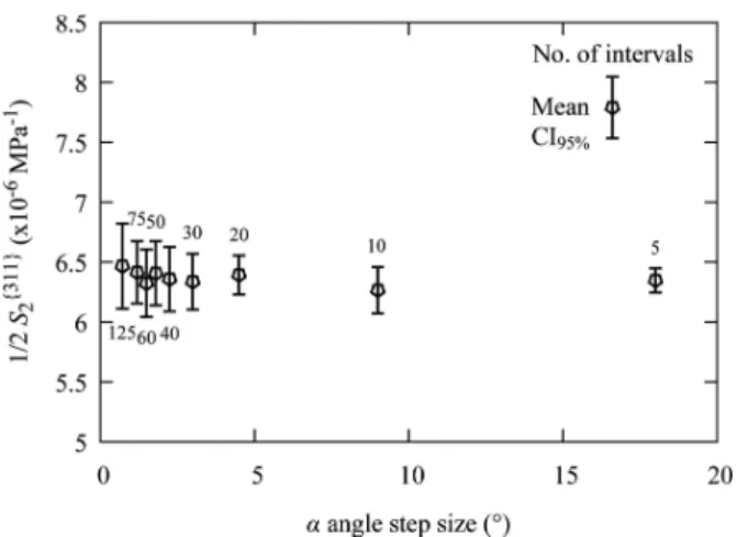
Figure 15
(a) XEC1
2Sf311g2 values calculated for the diffracting grains detected by the
2D detector at ' = 30'for 125 ! angles (from 0 to 90'). (b) Mean and
confidence interval (CI95%) of the XEC 12Sf311g2 values calculated for
different !-step sizes. The corresponding number of ! angles is presented below or above the error bar. CI95%is the lower bound of the 95%
confidence interval on the standard deviation.
Figure 14
Number of diffracting grains detected by the two linear detectors for nine ' angles and their corresponding XEC1
2Sf311g2 values calculated for the
confidence interval on the standard deviation of an assumed normal distribution, determined with a *2test (Hines et al., 2008). Thus, in this case, the XEC standard deviation is less
than 0.23, 10$6MPa$1at the 95% level of confidence.
For the 2D detector, the1
2Sf311g2 values were calculated for a
0.72' !-step size to characterize the ring geometry. The 125
XEC values determined for ' = 30'are presented in Fig. 15(a).
The values range from 5.89, 10$6to 6.92, 10$6MPa$1and
a mean value of 6.36, 10$6MPa$1 is observed, yielding a
CI95%of 0.19, 10$6MPa$1. This low !-step size implies five
times fewer diffracting grains per ! value than for a given ' position with the two linear detectors, resulting in a larger
range of the computed values but a lower CI95%value (as the
confidence interval is also based on the population size). Fig. 15(b) shows the mean and the confidence interval values of the XEC calculated for different !-step sizes. It can be observed that increasing the step size narrows the confidence interval CI95%, while the mean value remains almost constant.
Indeed, decreasing the number of intervals increases the number of orientations accounted for in one interval, which results in better approximation of the XEC.
Different ' angles have also been simulated for the 2D detector and 0.72'!-step size. The average XEC value and the
number of diffracting grains for the different ' angles are shown in Fig. 16. A quasi-constant number of diffracting grains can be observed throughout the entire range of simu-lated ' angles. The average XEC value slightly decreases for
high ' angles (a 0'' angle corresponds to a normal incident
X-ray beam).
For the linear detectors, the average XEC value of the diffracting grains is higher than the random texture XEC value, whereas for the 2D detector it is slightly lower. These differences are most likely to be due to the fact that the XEC is determined on sets of grains having a slight texture. The XEC values computed for the two detector types are not
Figure 16
Number of diffracting grains detected by the 2D detector for different ' angles and corresponding XEC1
2Sf311g2 values calculated for a 0.72'!-step
size (125 ! angles).
Figure 17
Orientation distribution maps of 1 in sample for the following reduction factors: (a) R = 1 (initial map), (b) R = 1/2, (c) R = 1/5, (d) R = 1/10, (e) R = 1/15 and ( f ) R = 1/20. Information on map maximum texture index and grain density (in grains mm$2) is also provided.
statistically different and seem not to be highly affected by the detector’s position, i.e. ' angle, in the case of homogeneous microstructure.
4.6. Effect of grain size
XRD measurement quality may suffer when a relatively small number of orientations are diffracting, leading to anisotropy inherent to the used XRD method. The grain size or grain density can therefore affect the XRD measurement. The effect of grain size on the XEC was studied by ‘artificially’ reducing the grain density. The initial EBSD map size was reduced while keeping the same irradiated zone area, decreasing the grain density. Five resized EBSD maps, using reduction ratios of R = 1/2, 1/5, 1/10, 1/15 and 1/20, were thus
investigated, providing grain densities ranging from 12 526 to
1232 grains mm$2. Note that the initial EBSD map grain
density is 25 316 grains mm$2(Table 5), corresponding to an
average grain size of 6mm (ASTM grain size number 12).
A 1/20 reduction ratio corresponds to a 20 times increase of
the grain size, giving a 120mm average equivalent diameter
(ASTM grain size number 3) or a grain density of 1232 grains mm$2.
Fig. 17 presents the different reduced maps as orientation distribution maps with respect to the RD. The map reduction was set to start from the upper-left corner of the initial EBSD map, shown in Fig. 17(a). The grain size was artificially increased by focusing the area of interest on a smaller portion of the initial map and by keeping the same scale. The IPFs have also been determined for each map and maximum texture indexes are reported in Fig. 17. It can be observed that increasing the average grain size slightly increases the maximum texture
index without creating a specific
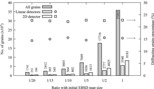
texture. Fig. 18 presents, for the six cases, the total number of grains and the total number of unique diffracting grains for both detectors. The number of grains is reduced from
35 805 (25 316 grains mm$2) to 1743
(1232 grains mm$2). Constant
percen-tages of diffracting grains were found for the linear detectors and the 2D detector, of 15 and 23%, respectively.
The calculated XEC was only
affected by the change in grain density, owing to the homogeneous grain orientation and grain-size distributions.
For the five resized maps, XEC 1
2S f311g 2
mean and confidence interval values were calculated for both diffractometer types and were compared with the results of the initial EBSD map (R = 1). The results are presented in Fig. 19. The
1 2S
f311g
2 values increase by up to 2.1% as
the grain density decreases, whereas the confidence interval significantly
broadens. For the 2D detector,
increasing the !-step size increases the number of grains taken into
considera-tion for each XEC computation,
broadening the confidence interval CI95%. When the number of diffracting
grains decreases significantly, the !-step size for analyzing the Debye ring has to
be increased to 1.2' to ensure the
presence of diffraction data for all ! intervals. For instance, in the case of
R = 1/20, the 1
2S f311g
2 values can only
be computed for an !-step size of 1.2'
or higher. The values vary from
Figure 18
Histogram of the number of grains for the different reduced maps and the corresponding diffracting-grain number for the linear and 2D detectors. The percentage of diffracting diffracting-grains is also plotted for both detector geometries.
Figure 19
Mean values and confidence interval on the standard deviation (CI95%) of the XEC 12Sf311g2
determined for the {311} planes of the diffracting grains detected by the linear and 2D detectors in the case of five resized maps. Results for the 2D detector are presented for 0.72 and 1.2'!-step sizes.
The CI95%values are computed from the lower bounds of the 95% confidence interval on the
5.16, 10$6 to 8.40, 10$6MPa$1, yielding a 0.58,
10$6MPa$1 confidence interval. The high CI95%values can
still be explained by the very low number of diffracting grains contributing to each XEC estimation. Therefore, a high !-step size should be used when large grains (or low grain density) are found in the material.
4.7. Effect of diffractometer oscillation
Experimentally, the number of diffracting grains can be increased by oscillating the X-ray beam in the ’ plane. Different oscillation values have been simulated around the ' position for both diffractometers using 1' oscillation steps,
meaning that for a ' = 25' position and a 2' oscillation the
X-ray beam and the detectors were oscillating from 23 to 27'.
The simulations were realized for the reduction ratios R = 1/15
and R = 1/20, corresponding to 90 and 120mm average grain
sizes, respectively. The low grain density allows only a small number of diffracting grains, yielding a broader XEC confi-dence interval. The results are presented in Fig. 20, and the values for the steady positions (presented in Figs. 18 and 19) are included as 0' oscillations. For both diffractometers, the
oscillations increase the number of diffracting grains detected
by the detectors. A 2' oscillation captures up to 55% more
diffracting grains for the 2D detector, whereas the linear detectors only capture up to 36% more grains. Increasing the
oscillation angle for the linear detectors does not significantly increase the total number of diffracting grains because the oscillation for a ' position ends up superimposing the oscil-lations of the other ' positions, hence the asymptotic curves. The XEC values tend to decrease with the oscillations for the 2D detector, while increasing for the two linear detectors. With oscillations, the confidence interval on the standard deviation is found to be narrower by up to 43 and 36% for the linear detectors and the 2D detector, respectively. For the two reduction ratios, the narrowest confidence intervals are found for 3 and 4' oscillations for the linear detectors and the 2D
detector, respectively.
4.8. Effect of inhomogeneous microstructure
A bimodal microstructure composed of a large number of
grains having a 6mm average grain size and very few grains
with a grain size higher than 100mm was found in the 3.5 in
sample, as depicted in Figs. 3 and 4(b). The XEC calculations for both microstructures are presented in Fig. 21(a) for the two linear detectors using nine ' angles. The average XEC and confidence interval values of the nine ' angles are 6.41, 10$6 and 0.33, 10$6 MPa$1, respectively, for the 3.5 in sample.
Figure 20
Total number of unique diffracting grains and XEC1
2Sf311g2 mean values
calculated for two different reduction factors (R = 1/15 and R = 1/20) and for measurements with both techniques in the case of oscillations in the ’ plane. The calculations for the 2D detector were performed using 1.2'
!-step sizes. The error bars represent the confidence interval on the standard deviation (CI95%).
Figure 21
Comparison of the XEC1
2Sf311g2 calculated for the 1 and 3.5 in samples for
(a) nine ' angles in the case of measurements with two linear detectors and (b) 125 ! angles for the 2D detector at ' = 30'.
The mean value is higher than that found for the 1 in sample and, more importantly, the confidence interval has broadened by 44%.
The XEC was also calculated for the 2D detector at ' = 30'
and for 125 ! angles. The XEC values computed for the 3.5 in sample are compared with those obtained for the 1 in sample in Fig. 21(b). The average value is also found to be higher than that of the 1 in sample value, 6.47, 10$6MPa$1, whereas the confidence interval of 0.36, 10$6MPa$1has nearly doubled.
Fig. 22 shows the XEC mean values for different !-step sizes for comparison with Fig. 15(b). As for the 1 in sample, the confidence interval narrows when the step size increases, but remains significantly higher.
5. Discussion
X-ray diffraction techniques for residual stress measurements are based on the information coming from the distinct sets of grains satisfying the conditions for diffraction. Each strain used for the determination of the macro-stress is an average of the grain deformation in the set of diffracting grains. Because of the specific crystal elastic anisotropy of the grains in the measurement direction, the elastic behavior of the diffracting grains may differ from the macroscopic behavior (Noyan & Cohen, 1987; Hauk, 1997). Consequently, the {hkl}-dependent XECs Sfhklg1 and 12Sfhklg2 have to be carefully measured or
computed. Sample texture is also known to play a major role in stress measurements and must be taken into account when computing the XEC (Hauk, 1997).
In the cases studied in this work, the two samples (homo-geneous and bimodal microstructures) do not exhibit strong textures (Fig. 5). Nonetheless, both types of detector create some ‘artificial’ texture, which differs from one detector to the other owing to the diffraction conditions, as shown in Fig. 11. The ‘artificial’ textures determined for the homogeneous sample can be significant when considering a measurement at a given ' angle or ! angle, for the linear detectors and the 2D
detector, respectively (visible in Figs. 12 and 13). These textures result in some variations in the estimated XEC1
2Sf311g2 .
Variations of up to 10% of the XEC value have been observed between the different sets of diffracting grains and the XEC value of the {311} planes computed for the Hill bound in the case of an isotropic material. This value reaches 18% for the 3.5 in sample and its bimodal microstructure, which also plays a role in the diffraction measurement. Indeed, the lower number of grains reduces the number of orientations taken into consideration, resulting in a wider confidence interval on the standard deviation of the estimated XEC for both tech-niques.
It has been shown that increasing the grain size of a homogeneous microstructure leads to a significant broadening of the confidence interval on the standard deviation. None-theless, the percentage of grains contributing to the diffraction stays almost constant for both diffractometers (Fig. 18). For an
average grain size of 90mm (R = 1/15) and above, the default
0.72'!-step size of the 2D detector is not sufficiently large to
gather diffraction data in all regions of the Debye ring.
Therefore the !-step size had to be increased to 1.2' to
compute the XEC for all ! steps.
The lack of diffraction data resulting from the diffraction texture or grain size can be overcome by the oscillation of the diffractometer around its ' position in the ’ plane (Fitzpatrick
et al., 2005). The simulations have shown that adding a 2'
oscillation to the measurement increases the number of diffracting grains by up to 55% for the 2D detector and 36% for the linear detectors. Further increase of the number of diffracting grains is limited by the superimposition of the ' positions for the sin2 method and the linear detectors, as it is a multi-angle-based method. Indeed, increasing the oscillation angle to more than half the angle between two ' inclinations (Table 3) would lead to diffracting grains contributing to the diffraction data of two diffraction vector sets. This would mean that the diffraction data of a grain could be used for the measurement of two different strains, i.e. two different points in the plot "fhklg’ versus sin2 , which may lead to inaccuracy in
the linear regression between "fhklg’ and sin2 , and therefore
an inaccurate stress determination. In both cases, the oscilla-tions narrow the confidence interval on the standard deviation of the estimated XEC, when compared with the intervals of the non-oscillating cases.
The low number of shared diffracting grains between the two methods (representing 20 and 14% of the total identified
diffracting grains for the sin2 and cos ! methods,
respec-tively) implies that the strains are measured from different sets of grains. These sets have different elastic behaviors, as observed in this study by the XEC variations, and may lead to the determination of different residual stresses.
Moreover, the residual stress measurement relies on the existence of a linear relationship between "fhklg’ or "fhklg! and the
sin2 or the cos ! values, respectively. Some authors (Hauk, 1997; Fitzpatrick et al., 2005) have shown that, when a low
number of exposures are considered in the sin2 method,
errors arise in the linear regression and the estimated residual stress values may be wrong. Even if the cos ! method
Figure 22
Mean and confidence interval (CI95%) of the XEC12Sf311g2 calculated for
different !-step sizes for the 3.5 in sample. The corresponding number of ! angles is presented below or above the error bar. CI95%is the lower
generates more points for the linear regression, a compromise between the number of diffracting grains for a given point and the number of points considered for the linear regression (i.e. the !-step size) should be found. In fact, for a small !-step size and in the case of a large grain microstructure (low number of diffracting grains), statistical effects will result in large varia-tions of the data "fhklg! used to estimate the residual stress
[equation (14)], leading to a significant error in the slope of the regression line used to compute the residual stress. Increasing the !-step size will reduce the statistical errors but also reduce the number of points available for the linear regression. There is then an opportunity to develop further the current approach to better specify the optimum conditions that will minimize the errors when estimating an actual residual stress field. Moreover, the presence of some crystallographic texture in a material could be taken into consideration as it is known to result in additional difficulties in estimating the actual residual stresses in a component.
6. Conclusions
The objective of this study was to compare the traditional X-ray diffraction technique for residual stress measurement,
i.e. the sin2 method, and the recently implemented cos !
method through the elastic properties of the diffracting grains. For this purpose, a MATLAB script has been developed to identify the diffracting grains and two EBSD maps were used to generate realistic distributions of orientation and grain size. The specificities of the two XRD residual stress measurement methods were taken into consideration and various para-meters were varied to better illustrate their effect on the quality of potential residual stress measurements. From the sets of identified diffracting grains, the following results have been observed:
(1) The 2D detector used by the cos ! method captures, in a single exposure, diffraction data from 1.5 times more unique diffracting grains than nine angular positions of the linear
detectors used in the sin2 method (acceptable number of
points allowing the determination of residual stresses via this
method). Increasing the number of ' angles in the sin2
method does not allow the same number of unique diffracting grains to be reached. Keeping a realistic time of X-ray expo-sure for residual stress meaexpo-surement purposes, nine expoexpo-sures are proposed with the consequence that about 50% fewer unique grains are diffracting.
(2) The ‘artificial’ crystallographic texture effect related to the two XRD methods has been calculated. It was shown that the two methods yield two different types of textures. Furthermore, the diffracting grains detected by the linear detector method generate a higher texture index than for the 2D detector, even if the nine incident ' angles are used (about 45% higher). Nonetheless, when considering the stress calcu-lation specificity of the cos ! method – division of the Debye ring into 125 ! angles – the highest texture index computed for the different ! angles is similar to that found for the linear detectors at a given tilt angle (' angle). Artifacts can arise
from the strong ‘artificial’ texture during residual stress computations.
(3) The detrimental effect of large grain size was simulated. It can be overcome by the oscillation of the diffractometer in the ’ plane. For the sin2 method, the oscillation angle should be carefully chosen so that it remains below half of the angle between two ' positions, otherwise a superimposition of the ' positions may occur, limiting the beneficial effect of this parameter. In addition to the oscillations, the cos ! method can use different !-step sizes to overcome the grain-size effects.
The variations in XEC could lead to a nonlinear regression for the residual stress computation and therefore a large error in the slope determination, resulting in an inaccurate residual stress measurement.
Future work could include textured materials, such as rolled aluminium alloy plates, to study the effect of material texture on the ‘artificial’ XRD texture and on the XEC.
Acknowledgements
DD would like to thank Dr Se´bastien Le Corre and Dr Benjamin Tressou for fruitful discussions.
Funding information
This work was financially supported by the Consortium of Research and Innovation in Aerospace in Quebec, the Natural Sciences and Engineering Research Council of Canada, Pratt & Whitney Canada, Bell Helicopter Textron, L3-Commu-nications MAS, Heroux Devtek, and Mathematics of Infor-mation Technology and Complex systems (grant No. RDC 435539-12).
References
Aba-Perea, P. E., Pirling, T., Withers, P. J., Kelleher, J., Kabra, S. & Preuss, M. (2016). Mater. Des. 89, 856–863.
ASTM International (2012). Standard Test Method for Residual Stress Measurement by X-ray Diffraction for Bearing Steels. ASTM Standard E2860-12. ASTM International.
ASTM International (2013). E112-13 Standard Test Methods for Determining Average Grain Size. ASTM Standard E112-13. ASTM International.
Bachmann, F., Hielscher, R. & Schaeben, H. (2011). Ultramicroscopy, 111, 1720–1733.
Cullity, B. D. (1956). Elements of X-ray Diffraction. Reading: Addison-Wesley Publishing Company.
Delbergue, D., Le´vesque, M. & Bocher, P. (2017). Proceedings of the 13th International Conference on Shot Peening, pp. 237–243. Montre´al, QC, Canada. https://shotpeening.org/ICSP/icsp-13.php. Delbergue, D., Texier, D., Le´vesque, M. & Bocher, P. (2016).
Proceedings of the 10th International Conference on Residual Stresses 2016 (ICRS-10), edited by T. M. Holden, O. Mura´nsky & L. Edwards, Materials Research Proceedings, Vol. 2, pp. 55–60. Millersville: Materials Research Forum.
Eatough, M. O., Rodriguez, M. A., Blanton, T. N. & Tissot, R. G. (1997). Adv. X-ray Anal. 41, 319–326.
Erinosho, T. O., Collins, D. M., Wilkinson, A. J., Todd, R. I. & Dunne, F. P. E. (2016). Int. J. Plast. 83, 1–18.
Etter, A. L. & Baudin, T. (2013). Rayonnement Synchrotron, Rayons X et Neutrons au Service des Matere´riaux, edited by A. Lodini & T. Baudin, ch. 6, pp. 278–321. Les Ulis: EDP Sciences.
Fitzpatrick, M., Fry, A., Holdway, P., Kandil, F., Shackleton, J. & Suominen, L. (2005). Determination of Residual Stresses by X-raye Diffraction. National Physical Laboratory, Teddington, UK. Frija, M., Hassine, T., Fathallah, R., Bouraoui, C. & Dogui, A. (2006).
Mater. Sci. Eng. A, 426, 173–180.
Garie´py, A., Bridier, F., Hoseini, M., Bocher, P., Perron, C. & Le´vesque, M. (2013). Surf. Coat. Technol. 219, 15–30.
Gna¨upel-Herold, T., Brand, P. C. & Prask, H. J. (1998). J. Appl. Cryst. 31, 929–935.
Guagliano, M. (2001). J. Mater. Process. Technol. 110, 277–286. Haldipur, P. (2006). PhD thesis, Iowa State University, USA. Hauk, V. (1997). Structural and Residual Stress Analysis by
Nondestructive Methods: Evaluation, Application, Assessment. Amsterdam: Elsevier.
He, B. B. (2009). Two-Dimensional X-ray Diffraction. Hoboken: J. Wiley & Sons.
Heydari Astaraee, A., Miresmaeili, R., Bagherifard, S., Guagliano, M. & Aliofkhazraei, M. (2017). Mater. Des. 116, 365–373.
Hielscher, R. (2013). J. Multivariate Anal. 119, 119–143. Hill, R. (1952). Proc. Phys. Soc. Sect. A, 65, 350–354.
Hines, W. W., Montgomery, D. C., Goldsman, D. M. & Borror, C. M. (2003). Probability and Statistics in Engineering, 4th ed. Hoboken: John Wiley & Sons.
Hiratsuka, K., Sasaki, T., Seki, K. & Hirose, Y. (2003). Adv. X-ray Anal. 46, 61–67.
Ho¨rz, F. & Quaide, W. L. (1973). Moon, 6, 45–82. Howard, C. J. (1982). J. Appl. Cryst. 15, 615–620.
Klotz, T., Delbergue, D., Bocher, P., Le´vesque, M. & Brochu, M. (2018). Int. J. Fatigue, 110, 10–21.
Klotz, T., Miao, H. Y., Bianchetti, C., Le´vesque, M. & Brochu, M. (2018). Int. J. Fatigue, 113, 204–221.
Kocks, U. F., Tome´, C. N. & Wenk, H. R. (1998). Texture and Anisotropy: Preferred Orientations in Polycrystals and Their Effect on Materials Properties. Cambridge University Press.
Kohri, A., Takaku, Y. & Nakashiro, M. (2016). Proceedings of the 10th International Conference on Residual Stresses 2016 (ICRS-10)}, edited by T. M. Holden, O. Mura´nsky & L. Edwards, Materials Research Proceedings, Vol. 2, pp. 103–108. Millersville: Materials Research Forum.
Ledbetter, H. M. & Reed, R. P. (1973). J. Phys. Chem. Ref. Data, 2, 531–618.
Mainprice, D., Hielscher, R. & Schaeben, H. (2011). Geol. Soc. London Spec. Publ. 360, 175–192.
Margetan, F., Nieters, E., Haldipur, P., Brasche, L., Chiou, T., Keller, M., Degtyar, A., Umbach, J., Hassan, W., Patton, T. & Smith, K. (2005). Fundamental Studies of Nickel Billet Materials–Engine Titanium Consortium II. Technical Report. US Department of Transportation, Washington, DC, USA.
Miyazaki, T. & Sasaki, T. (2016). J. Appl. Cryst. 49, 426–432. Murray, C. E. (2013). J. Appl. Phys. 113, 153509.
Noyan, I. C. & Cohen, J. B. (1987). Residual Stress Measurement by Diffraction and Interpretation. New York: Springer-Verlag. Peterson, N., Kobayashi, Y. & Sanders, P. (2017). Proceedings of the
13th International Conference on Shot Peening, pp. 80–86. Montre´al, QC, Canada. https://shotpeening.org/ICSP/icsp-13.php. Preve´y, P. S. (1986). Materials Characterization, Vol. 10, pp. 380–392.
Materials Park: ASM International.
Preve´y, P. S. (2000). Proceedings of the 20th ASM Materials Solution Conference and Exposition. St Louis, Missouri, USA.
Ramirez-Rico, J., Lee, S.-Y., Ling, J. J. & Noyan, I. C. (2016). J. Mater. Sci. 51, 5343–5355.
Ruud, C. (2002). Handbook of Residual Stress and Deformation of Steel, edited by G. Totten, M. Howes & T. Inoue, pp. 99–117. Materials Park: ASM International.
SAE International (2003). Residual Stress Measurement by X-ray Diffraction. Standard SAE HS784. SAE International.
SAE International (2009). Nickel Alloy, Corrosion and Heat-Resistant, Bars, Forgings, and Rings 52.5Ni–19Cr–3.0Mo–5.1Cb (Nb)–0.90Ti–0.50Al–18Fe Consumable Electrode or Vacuum Induction Melted 1775'F (968'C) Solution and Precipitation Heat
Treated. Standard SAE AMS5663M. SAE International. Sasaki, T. (2014). Mater. Sci. Forum, 783–786, 2103–2108.
Sasaki, T., Hirose, Y., Sasaki, K. & Yasukawa, S. (1997). Adv. X-ray Anal. 40, 588–594
Schajer, G. S. (2013). Practical Residual Stress Measurement Methods. Chichester: Wiley.
Taira, S., Tanaka, K. & Yamasaki, T. (1978). J. Soc. Mater. Sci. Jpn, 27, 251–256.
Tanaka, K. (2018). J. Appl. Cryst. 51, 1329–1338.
Tu, F., Delbergue, D., Klotz, T., Bag, A., Miao, H. Y., Bianchetti, C., Brochu, M., Bocher, P. & Levesque, M. (2018). Int. J. Mech. Sci. 145, 353–366.
Tu, F., Delbergue, D., Miao, H. Y., Klotz, T., Brochu, M., Bocher, P. & Le´vesque, M. (2017). Surface Coatings Technol. 319, 200–212. Van Houtte, P. & De Buyser, L. (1993). Acta Metall. Mater. 41, 323–
336.