HAL Id: hal-02393128
https://hal-mines-paristech.archives-ouvertes.fr/hal-02393128
Submitted on 4 Dec 2019
HAL is a multi-disciplinary open access
archive for the deposit and dissemination of
sci-entific research documents, whether they are
pub-lished or not. The documents may come from
teaching and research institutions in France or
abroad, or from public or private research centers.
L’archive ouverte pluridisciplinaire HAL, est
destinée au dépôt et à la diffusion de documents
scientifiques de niveau recherche, publiés ou non,
émanant des établissements d’enseignement et de
recherche français ou étrangers, des laboratoires
publics ou privés.
Urban Energy Models Validation in Data Scarcity
Context: Case of the Electricity Consumption in the
French Residential Sector
Thomas Berthou, Bruno Duplessis, Pascal Stabat, Philippe Rivière,
Dominique Marchio
To cite this version:
Thomas Berthou, Bruno Duplessis, Pascal Stabat, Philippe Rivière, Dominique Marchio. Urban
Energy Models Validation in Data Scarcity Context: Case of the Electricity Consumption in the
French Residential Sector. Building Simulation 2019, Sep 2019, Rome, Italy. �hal-02393128�
Urban Energy Models Validation in Data Scarcity Context: Case of the Electricity
Consumption in the French Residential Sector
Thomas Berthou
a, Bruno Duplessis
a, Pascal Stabat
a, Philippe Rivière
a, Dominique Marchio
aa
MINES ParisTech, PSL - Research University, CES - Centre for energy efficiency of systems, 60
Bd St Michel 75006 Paris, France
Abstract
Urban energy models (UEM) are useful to evaluate energy efficiency policies at district or city scale and to make the best decisions in terms of financial and environmental impacts. Probabilistic and simple physical models coexist in the UEM often with several dozens of parameters per building. Parameters coming from different databases with no consistency in the levels of uncertainty make the necessary validation difficult. This article proposes a method as a first attempt to validate UEM in a data scarcity context which requires only the annual electricity consumption of several carefully chosen cities.
The first step aims to identify one parameter per energy end-use which has the largest impact on the energy consumption and the highest uncertainty. The second step aims to calibrate the model at country scale or at large territory scale to set parameters’ values. The third step consists in selecting several cities (inside the territory previously used for calibration) to evaluate particular aspects of the UEM. The last step aims to simulate the calibrated model on the selected cities and to compare the simulation with the energy consumption information.
The method is illustrated through the case of the electricity consumption in the French residential building sector with Smart-E, a bottom-up UEM tool.
Introduction
The Paris agreement (COP21) shows that most countries want to reduce their greenhouse gas emissions to contain the climate change. In Europe, the building sector represents 40% of the total energy consumption and 36% of greenhouse gas emissions1, which is why regulations
strongly encourage countries, regions and cities to set up energy efficiency measures in the building sector. To evaluate the impact of specific energy efficiency measures (e.g. building renovation, new appliances, demand side management) new simulation tools are needed. These tools exist (Frayssinet et al., 2017) and are adapted to different scales, simulation time steps, building types and energy efficiency measures. To be used in a real territory for energy efficiency strategy comparison, these models need to be validated, at least at
1
http://ec.europa.eu/energy/en/topics/energy-efficiency/buildings
an aggregated level of simulation. Since the number of simplifying assumptions is high they can hardly be validated one by one and the impact on the energy consumption is difficult to evaluate. Below are several examples of assumptions frequently used in bottom-up UEM having a significant impact on the simulation results:
air infiltration rate is chosen from standard values
temperature set-points are chosen from probabilistic distributions
buildings or dwellings are represented as a reduced number of thermal zones
activity profiles follow patterns and come from stochastic models or time tables
household appliances (washing machines, TV, computers,…) are assigned with probabilistic distributions
One solution to validate UEM is to compare results from simulation to energy consumption measured on real territories. Table 1 presents previous works on bottom-up simulation frameworks for the simulation of energy in cities and the validation methodology used by the authors. This literature review shows that annual and monthly energy error is commonly used as a criteria for validation, even if most UEM are dynamic.
Yeo et al. (2013), Nouvel et al. (2017) and Sokol et al. (2017) have a slightly different approach by using wider territory: a complete city (eg. 22 adjacent districts); but less data for validation. Indeed, annual or monthly consumption values are measured and used for performance criteria calculation. These studies show a good match between models and real territories but the energy end-use models (equations or parameters) that should be improved are not known.
Widen et al. (2009) and Fischer et al. (2015, 2016) go further by using criteria which assess daily and intra-day performances of the UEM. Data used for validation is coming from measurement campaigns on a reduced number of buildings or households, all situated in the same area. These methods for UEM validation are permitted thanks to a large campaign with short time step measurement allowing few limitations in the validation process. By avoiding compensation of errors
between days or periods in the day, this validation method enables a better evaluation of UEM parameters. Tanigushi et al. (2016) have an original approach by validating their UEM at a regional scale by comparing the model outputs with 1237 households electric load curve randomly selected among 8.6 million households from the simulated region. Once again, this validation method is possible only by having access to the results of a large monitoring campaign.
Method
This study suggests a repeatable method as a first step to validate a bottom-up UEM at city scale in a context of data scarcity. The required information are the aggregated annual energy consumption (e.g. electricity bills) for several cities and the annual consumption for each energy end-use at larger territory scale (e.g. country) which contains the cities. The particularity of this approach is to compare the UEM outputs with the energy consumption of several real cities carefully chosen to represent the national diversity in terms of households and dwellings characteristics. The comparison is made after a calibration process realized at the country scale on each energy use. All necessary information needed to realize the validation process could be found freely in many territories where open-data are easily available.
This article introduces a four steps methodology: Step 1 - To identify the model parameters which have the largest impact on the energy consumption and the highest uncertainties. These parameters will be used for calibration. Ideally, one parameter per energy use should be selected. This selection may be conducted through a screening method or from a review of literature. In this article, we chose the review of literature since the range of uncertainties is difficult to evaluate for some of the UEM parameters in the screening method.
Step 2 - To calibrate the model at country scale or at large territory scale with the selected parameters. Indeed, it is often at this scale that statistics on energy consumption are known. For example, Almeida et al. (2011) give average annual end-use electricity consumption for 12 European countries; this type of information is thus available at large scale but may not be available at the scale of the UEM. In addition, since simulating a complete country with tool designed for city scale can be a challenge, a method to reduce the computation time is suggested.
Step 3 - To select specific cities (inside the territory used for calibration) in order to evaluate particular aspects of the city model. Several criteria can be selected depending on the modelled end-use and the available information for these cities. In our case, we use the following characteristics:
proportion2 of houses or apartments
2
the proportion are unitary (eg. number of single-family houses divided by the total number of dwellings)
proportion of rich or poor households
proportion of ancient constructions or new constructions
proportion of heating systems using electricity Cities close to national mean values and cities with extreme values (e.g. minimum presence of electric heating systems in the city) are chosen in this article. Note that since these characteristics can be strongly correlated among themselves only their combined impact is explored here.
Step 4 - To simulate the calibrated model on the selected cities and to compare the simulation with their energy consumption information (e.g. electricity bills). The errors can be analyzed to identify possible sources and thus improvement paths of the UEM.
This method will be illustrated with Smart-E, a general bottom-up UEM framework for the French building sector (Berthou et al., 2015). Only the residential electric consumption is considered in this work but the same method can be used for natural gas consumption, district heating and fuel consumption validation in the residential or the commercial building sectors.
Presentation of Smart-E UEM
Smart-E is a bottom-up simulation platform designed to evaluate energy efficiency strategies. Databases and simple physical and probabilistic models are used to simulate the main energy uses in dwellings. All algorithms are written with Python programming language and Numpy+Pandas Packages. Figure 1 shows the inputs - outputs and the main sub-models of Smart-E. Figure 2 presents the electric consumption of a small city during two working days in winter. This figure illustrates how Smart-E sums consumption from different types of models to reconstruct global electric load of dwellings. Each dwelling load is different and this leads to a realistic diversity of consumption profiles.
Model description
Since some parameters come from stochastic models where the values are highly uncertain, choice has been made to use simple envelope or system physical models for city simulation. Therefore the complexities of the models are adapted to city or district simulation and not to single building or dwelling simulation.
Heating systems and envelope models
Thermal needs of dwellings are calculated with a two thermal zones model, one for the living space (living room, kitchen, bedrooms) and another one for spare rooms where heaters are turned off or temperature set point lowered. A second order differential equation (2 capacities and 6 resistances) is used for each thermal zone modeling which has been validated for HVAC consumption in buildings (Berthou et al., 2014). With only 10 parameters per thermal zone, the model is quickly configurable from easy to find information on dwellings (e.g. floor area, built year, windows to wall ratio, orientation).
Table 1: Comparison of validation methods for UEM Authors Simulation
scale
UEM Time
step Data for validation Criteria for validation Widen et al., 2009 Household to
country 1 h
Hourly electric consumption of each appliance (217 households)
Error on mean daily electricity demand per household and per
appliance Yeo et al., 2013 District to large
city 1 h
Monthly energy consumption of an
existing city Monthly energy error Nouvel et al., 2017 District to large
city 1 y
Annual gas consumption for 22
districts, 5 years Annual energy error for 22 districts Fonseca &
Schlueter, 2015 Building to city 1 h
Annual electricity, space cooling and heating consumption
Annual energy error for 23 buildings (electricity, heating and cooling) Taniguchi et al.,
2016
Building to
district 1 h
Hourly electricity consumption
(1237 households) Intra-day electricity load curve error Fischer et al., 2015
and 2016
District to
country 15 min
Hourly electricity consumption (430 households)
Annual to dayly energy error, load profiles
Sokol et al., 2017 Building to city - Monthly electricity and gas consumption (2600 homes)
Energy distribution error (monthly to annually comparisons)
This article District to
country 10 min
Annual electricity consumption for
households in ten cities Annual energy error for 10 cities
Figure 1: Data flow and model coordination in Smart-E
Figure 2: 2 days electric consumption for 4000 dwellings during winter only 22% of dwellings use electric heating systems, 10 min simulation time step (Smart-E)
The window’s opening is simulated by changing the airflow rate and the solar protection closing effect by reducing the solar flux power on the windows. Heat emitters are modelled using a first-order differential equation (1 capacity and 1 resistance). Static parameters of heat emitters are calculated from reference values for each technology.
Domestic hot water (DHW)
Time of use (ToU) data (INSEE, 2009) is used to simulate hot water consumption associated with activities presented in table 2. A hot water volume associated with an electric water heating system is simulated as a homogeneous water volume depending on the area of dwellings. Electric DHW systems can receive orders from the grid to force heating start-up depending on the city localization. We assume that 85% of the storage electric water heaters are hourly controlled and the other 15% can start at any time during the day when the internal tank temperature becomes too low.
Lighting
Lighting consumption is calculated from the French national building code (CSTB, 2010). Dwelling indoor illumination is calculated from weather and geometrical information then a piecewise linear function gives the light surface ratio from the illumination value.
Other electric appliances
ToU data is used to describe occupants’ activities and generate weekly timetables. Each occupant who interacts with the energy consumption in the dwelling is simulated during one week. Then the same week is repeated all the year (a weekly organization of the households is assumed). Occupants have eight possible activities (table 2) and can do up to two activities at a time with exceptions (no possible to sleep and to eat for instance). For each activity and each household electrical power is calculated from a statistical distribution. The mean power of each type of electric appliance is calculated during the calibration process.
“Dishwashing” and “laundry” activities are differentiated from the others because occupants can do other activities when those are not handmade. The refrigeration, stand-by and ventilation electric consumption are calculated with a stochastic model from field measurements.
Table 2: Activities of the ToU survey Activity
Name Details Type of consumption Digital
TV, computer, video game, DVD
player, phone
Electricity consumption Cooking Cooking plate,
microwave, oven...
Hot water, gas and electricity consumption Meal Action of eating None Dishwashing Cleaning the dishes
Hot water, electricity consumption (if
dishwasher) Laundry Taking care of
laundry (washing,
Electricity consumption (programmable)
drying) Rest Nap and sleep
Lighting turn off Temperature set point
reduction Personal car Bath, shower, body
care, Hot water consumption Other Game, homework,
reading… Electricity consumption
Data for model parameterization
This section outlines the main databases used in Smart-E for model parameterization.
National housing census
The French national census on housing and household description is used for dwelling description (INSEE, 2016). The census information and the interaction with models’ parameters are described in table 3. Information is available for 100% of dwellings in small cities (less than 10 000 inhabitants) and only 40% for medium and large cities.
Table 3: Example of national census information used by Smart-E
Census information Models Used Dwelling construction
year
Envelope performance, retrofit probability
Dwelling area walls surfaces, heated area Energy for heating Type of HVAC system Household composition
(age, activities)
Appliances used, hot water system, internal heat gain Single or multi-housing Heat losses area
Localization Weather data Time of use survey (ToU)
The French ToU survey is used to simulate occupants’ activities (INSEE, 2009). The database is composed of 19000 record sheets of 24 hours with more than 100 possible activities lasting 10 minutes at least. Wilke et al. (2013) created a global probabilistic model of household activities with the same survey conducted 10 years earlier from which household electric power profiles are simulated. In this paper, a similar but simpler approach is used. Instead of using a specific model, a one-week timetable from the concatenation of 24 hours record sheets is built for each occupant. Working days and weekends are respected and inhabitant main activity (worker, student, unemployed, retired, and other) are factored as well. At an aggregated level, the results are close to Wilke’s probabilistic model. The survey activities are sorted out in eight classes presented in table 2. The advantage of this approach is to respect a strict coherence between activities, for example there is no lighting or water consumption when nobody is at home.
Geographic information system (GIS)
GIS database (IGN, 2016) contains the geometrical descriptions of cities (e.g. buildings shape and height). In Smart-E the GIS data helps to better evaluate all parameters linked to geometrical information: shading
coefficient for each building, compactness and external surface for heat loss calculation.
Weather data
Outdoor temperature and solar radiation from the national weather company are used. One-hour time step measurements from more than 500 meteorological stations are available in the French territory.
Model calibration at country scale
Models are calibrated at country scale because information about annual consumption per energy use is often only available at this scale. This information is coming from statistical studies (eg. sells information, survey) and local monitoring campaigns (RTE, 2015). Uncertainty values related to these data are not known but ideally they should be incorporated to the calibration process. Weather data representative of the French 2012 weather are used for this simulation.
To keep the computation cost as low as possible only 10 000 real dwellings representative of national diversity are selected to be simulated. This reduced dwelling stock (RDS) is created by randomly selecting the dwellings in a national census database and verifying with specific criteria if the RDS has common statistic characteristics with the country scale information. Table 4 compares the reduced and the complete dwellings stock with selected parameters and shows a good match between both.
Table 4: Validation result of the RDS
Parameters Target values (Eq.1) RE Dwellings type Collective : 39.8%
Detached : 59.5%
<5% Main energy for heating
Electricity : 31.2% Natural gas : 35.9%
Fuel : 12.5% District heating : 4.6% mean occupant per dwelling 2.24
mean surface of dwelling 95 m²
Nine parameters are selected for the calibration process (one per energy-end-use). Eight of them are easy to choose since there is one candidate per energy use with high level of uncertainty: the mean electric power of electric appliances (or activities) and the mean hot water flow rate for DHW are therefore identified during the calibration phase. However, there are several candidates for heating need calibration which are highly uncertain and have a strong impact on heating needs. Booth et al. (2012) present a factorial sampling analysis to rank the input parameters from the most dominant to the less dominant and from the most uncertain to the less uncertain for heating energy consumption at an aggregated scale. For each parameter known to have a large impact on heating consumption, we verify with qualitative analysis if low-uncertainty value is known in Smart-E. From table 5, the air leakage seems to be the best candidate for the calibration process since only an
average value is known. Coefficient of performance for heating systems could also have been a good candidate but in France 95% of electric heating systems are electric convectors with a 100% efficiency.
Table 5: Possible parameters for heating consumption calibration Selected parameters from Booth et al. , 2012 Uncertainty level in Smart-E References Fraction of space heated Low Adapted correlation (Loga, et al., 2004) Internal heating
set−point temperature Medium
Distribution from national study (ADEME, 2013) Coefficient of performance for heating systems Very high Only 5% of heat pump in France (ADEME, 2013) Double−glazing U−value Low National building code (CSTB, 2010) Window−to−wall ratio Medium National survey
(INSEE, 2016) Percentage of glazing
that is double−glazed Medium
National survey (INSEE, 2016) External wall U−value Medium National building
code (CSTB, 2010) Single−glazing
U−value Low
National building code (CSTB, 2010) Air leakage and
ventilation Very high
Average value (Dimitroulopoulou,
2012) Once the parameters for the calibration process are chosen, a heuristic method is used to identify the values satisfying the national annual energy consumption of each energy use. It is to be noted that the parameters are correlated since the electric appliance consumption determine the internal gains, which have an impact on heating needs. The result of the calibration process is shown in table 6.
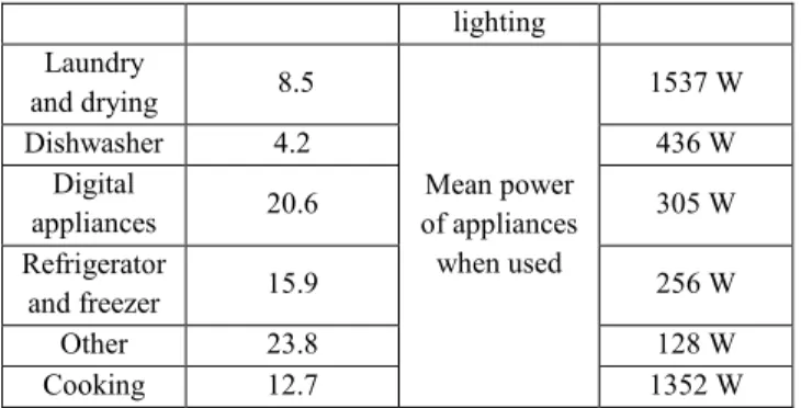
Table 6: Summary of the calibration process: energy objectives, tuned parameters and values after calibration
Energy end-use Annual electric consumption at country scale in 2012 (TWh) (RTE, 2015) Parameter to tune Parameter value after calibration
Heating 42.8 Annual mean air leakage 0.4 volume/hour Domestic hot water 20.6 Mean hot water consumption flow when used (60°C) 0.6 l/min
Lighting 9.5 Mean surface
lighting Laundry and drying 8.5 Mean power of appliances when used 1537 W Dishwasher 4.2 436 W Digital appliances 20.6 305 W Refrigerator and freezer 15.9 256 W Other 23.8 128 W Cooking 12.7 1352 W
Model validation at city scale
Ten cities located in the French Ile-de-France (IdF) region (12 million inhabitants) are manually selected for the model validation process. They are chosen to illustrate the diversity of the French architecture, social diversity and heating systems characteristics. For each city, the annual electric consumption of dwellings is known from 2012 electricity bills. For privacy reasons city names are not disclosed and only a proportion or average values of city characteristics are given.
A1, A2 and A3 are classic medium size French cities with a historic center and a more recent suburb. They are characterized by a large diversity in term of architecture, inhabitants, income and heating systems. These 3 cities are chosen to be individually representative of the national statistics for one or several parameters:
A1 in terms of income and proportion of electric heater and collective dwellings,
A2 in terms of construction year distribution and inhabitants activities distribution,
A3 to have close values for each indicator except for construction year statistics.
B1 and B2 are cities with a large majority of collective dwellings in very densely populated urban area. B1 is one of the richest territories in IdF and B2 is one of the poorest. By selecting these territories, UEM capability to take into account the impact of living standards on energy consumption can be assessed.
C1 has the particularity to be a very recent city with 88% of the dwelling built after 1990. By selecting this territory we should be able to discuss if the new dwellings are well simulated, especially their heating needs.
D1 and D2 are characterized with a high proportion of detached dwellings. The difference of thermal behaviors between detached and collective dwellings is well known and should be represented in the simulation tools (eg. compactness, area, heating systems, household composition).
E1 and E2 have the particularity to contain a low rate of electric heating system (less than 2%). These two cities will help us to validate the electricity consumption from electric appliances.
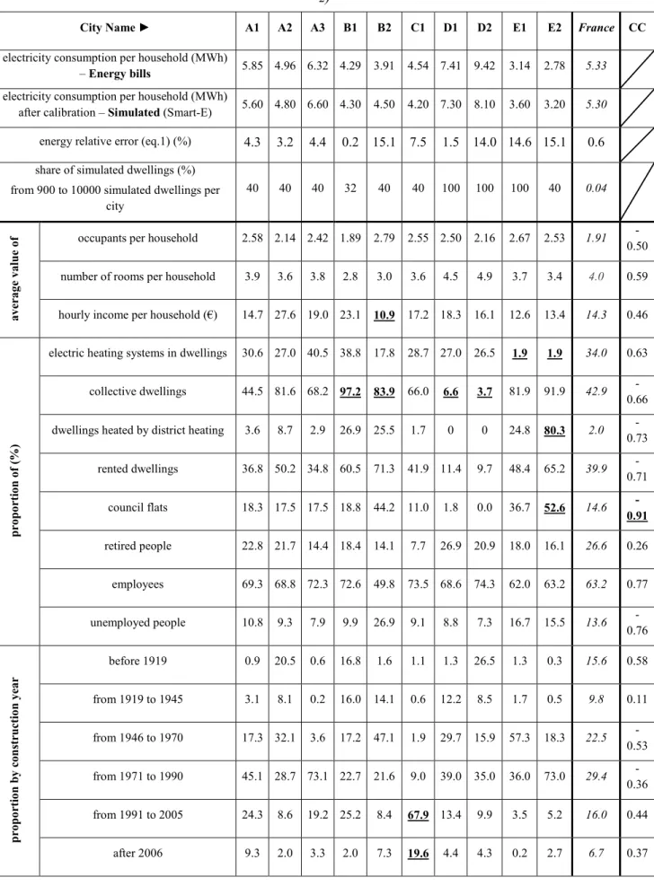
Table 7 shows that each city has interesting statistical characteristics to help us validate one or several aspects of the model. Definitive conclusion from the comparison
between simulated and energy consumption information cannot be made since the selected cities do not allow to fully separate a specific phenomena. However, this comparison helps us to identify weaknesses in the UEM and to decide where the development efforts must be focused. In the case study all the cities selected for the model validation are within a 100 km radius, so, only 4 well located meteorological stations (in 4 cities) for outdoor temperature and 1 for solar flux measurement are used for the simulations.
Results and discussion
Each city is simulated with Smart-E with the parameters calculated from the calibration process, then results from simulation are compared with annual electricity bills. The simulations are made with an INTEL XEON® CPU (3.5 GHz) and 64 Go of RAM, each simulation lasts around 5 minutes. From the comparison between simulation outputs and annual energy bills, we can see that:
The absolute error for all cities is below 1% (error on the sum of all cities simulated energy). This shows that the errors are compensated at 10 cities scale, which is expected since the simulation tool has been calibrated at large territory scale.
6 cities are well represented for annual electricity consumption with a relative error below 10%. 4 cities (B2, D2, E1 and E2) have a relative error
above 10%. Here the model may be perfectible and a detailed analysis is realized afterwards.
To go further in the analysis, the correlation coefficients (CC) between the absolute error and cities characteristics are calculated (eq. 2) and correlation values above 0.8 are especially analyzed in this case study to identify end-use models or parameters to be improved.
Table 7 shows one CC value above 0.8, it refers to the proportion of council flats. These results give an indication to choose which part of the model has to be improved first.
In the case study, the energy consumption of electric appliances in council flats might be examined to find ways of improvement (there is no electric heating systems in the studied council flats). Indeed, the UEM tends to overestimate the electric consumption in council flats. The first step should be to confirm the initial hypothesis that inhabitants of council flat have the same energy end-use habits and the same domestic equipment level than inhabitants of private flats.
Other correlation values show no evidence of model weakness in dwelling shape representation (collective or detached dwellings) or built year representation. Moreover household specificities seemed to be well taken into account by the UEM since the correlation coefficient is low for the “hourly income per occupant” or the “proportion of retired people”.
Table 7: Simulation results and statistical description of the 10 cities, comparison with the national average (2012), extreme values are in “bold”, CC is the correlation coefficient between simulation error and cities characteristics (eq.
2)
City Name ► A1 A2 A3 B1 B2 C1 D1 D2 E1 E2 France CC electricity consumption per household (MWh)
– Energy bills 5.85 4.96 6.32 4.29 3.91 4.54 7.41 9.42 3.14 2.78 5.33 electricity consumption per household (MWh)
after calibration – Simulated (Smart-E) 5.60 4.80 6.60 4.30 4.50 4.20 7.30 8.10 3.60 3.20 5.30 energy relative error (eq.1) (%) 4.3 3.2 4.4 0.2 15.1 7.5 1.5 14.0 14.6 15.1 0.6 share of simulated dwellings (%)
from 900 to 10000 simulated dwellings per city 40 40 40 32 40 40 100 100 100 40 0.04 av er ag e va lu e
of occupants per household 2.58 2.14 2.42 1.89 2.79 2.55 2.50 2.16 2.67 2.53 1.91 0.50
-number of rooms per household 3.9 3.6 3.8 2.8 3.0 3.6 4.5 4.9 3.7 3.4 4.0 0.59 hourly income per household (€) 14.7 27.6 19.0 23.1 10.9 17.2 18.3 16.1 12.6 13.4 14.3 0.46
p ro p or ti on o f (%)
electric heating systems in dwellings 30.6 27.0 40.5 38.8 17.8 28.7 27.0 26.5 1.9 1.9 34.0 0.63 collective dwellings 44.5 81.6 68.2 97.2 83.9 66.0 6.6 3.7 81.9 91.9 42.9
-0.66 dwellings heated by district heating 3.6 8.7 2.9 26.9 25.5 1.7 0 0 24.8 80.3 2.0
-0.73 rented dwellings 36.8 50.2 34.8 60.5 71.3 41.9 11.4 9.7 48.4 65.2 39.9 -0.71 council flats 18.3 17.5 17.5 18.8 44.2 11.0 1.8 0.0 36.7 52.6 14.6 -0.91 retired people 22.8 21.7 14.4 18.4 14.1 7.7 26.9 20.9 18.0 16.1 26.6 0.26 employees 69.3 68.8 72.3 72.6 49.8 73.5 68.6 74.3 62.0 63.2 63.2 0.77 unemployed people 10.8 9.3 7.9 9.9 26.9 9.1 8.8 7.3 16.7 15.5 13.6 -0.76 p ro p or ti on b y co n str u ctio n y ea r before 1919 0.9 20.5 0.6 16.8 1.6 1.1 1.3 26.5 1.3 0.3 15.6 0.58 from 1919 to 1945 3.1 8.1 0.2 16.0 14.1 0.6 12.2 8.5 1.7 0.5 9.8 0.11 from 1946 to 1970 17.3 32.1 3.6 17.2 47.1 1.9 29.7 15.9 57.3 18.3 22.5 -0.53 from 1971 to 1990 45.1 28.7 73.1 22.7 21.6 9.0 39.0 35.0 36.0 73.0 29.4 -0.36 from 1991 to 2005 24.3 8.6 19.2 25.2 8.4 67.9 13.4 9.9 3.5 5.2 16.0 0.44 after 2006 9.3 2.0 3.3 2.0 7.3 19.6 4.4 4.3 0.2 2.7 6.7 0.37
Conclusion
On-site measurements are necessary to validate UEM and since it is time consuming and expensive to monitor the energy consumption at city scale, a methodology based on aggregated energy bills has been presented to validate UEM outputs on an annual basis. After the UEM calibration at country scale, simulation results have been compared to annual electricity consumption of 10 chosen cities:
classic medium French cities, rich and poor cities (on average),
cities with a majority of collective or detached dwellings,
cities with little electric heating systems, a recent city.
The case study shows a good match between Smart-E and the energy bills on 6 cities. On the other hand, 4 cities have an absolute error above 10% on total annual electric consumption which shows ways of improvement. A correlation between “simulation errors” and “proportion of council flats” suggests that the model for electric appliance simulation in council flats should be improved.
This method can be adapted according to local energy context and UEM specificities.
Acknowledgment
We would like to thank the ARENE Ile-de-France for sharing the data used in the validation process.
References
ADEME, 2013. Baromètre 10 000 ménages : Les ménages français face à l'efficacité énergétique de leur logement. Agence de l'Environnement et de la
Maîtrise de l'Energie.
Almeida, A., Fonseca, P., Schlomann, B. & Feilberg, N., 2011. Characterization of the household electricity consumption in the EU, potential energy savings and specific policy recommendations. Energy and
Buildings, Issue 43.
Berthou, T. et al., 2015. Smart-E: a tool for energy demand simulation and optimization at the city scale.
Building Simulation 2015.
Berthou, T., Stabat, P., Salvazet, R. & Marchio, D., 2014. Development and validation of a gray box model to predict thermal behavior of occupied office buildings. Energy and Buildings, Volume 74. Booth, A. T., Choudhary, R. & Spiegelhalter, D. J.,
2012. Handling uncertainty in housing stock models.
Building and Environment, Issue 48.
CSTB, 2010. Réglementation thermique 2012. Centre
scentifique et technique du bâtiment.
Dimitroulopoulou, C., 2012. Ventilation in European dwellings: A review. Building and Environment, Issue 47.
Fischer, D., Hartl, A. & Wille-Haussmann, B., 2015. Model for electric load profiles with high time
resolution for German households. Energy and
Buildings, Issue 92.
Fischer, D., Wolf, T., Scherer, J. & Wille-Haussmann, B., 2016. A stochastic bottom-up model for space heating and domestic hot hotwater load profiles for German households. Energy and Buildings, Issue 124.
Fonseca, J. A. & Schlueter, A., 2015. Integrated model for characterization of spatiotemporal building energy consumption patterns in neighborhoods and city districts. Applied Energy, Issue 142.
Frayssinet, L. et al., 2017. Modeling the heating and cooling energy demand of urban buildings at city scale. Renewable and Sustainable Energy Reviews, Issue 81.
IGN, 2016. BDTOPO. [online, 12/04/2018] http://professionnels.ign.fr/.
INSEE, 2009. Time of use survey. [online, 12/04/2018]
http://www.insee.fr/.
INSEE, 2016. fichiers détail du recensement de la population 2013. [online, 12/04/2018] http://www.insee.fr/.
Loga, T., Grobklos, M. & Knossel, J., 2004. Der Einfluss des Gebäudestandards und des Nutzerverhaltens auf die Heizkosten. INSTITUT
WOHNEN UND UMWELT.
Nouvel, R., Zirak, M., Coors, V. & Eicker, U., 2017. The influence of data quality on urban heating demand modeling using 3D city models. Computers,
Environment and Urban Systems, Issue 64.
RTE, 2015. Bilan prévisionnel de l'équilibre offre-demande d'électricité en France. [online, 12/04/2018]
http://www.rte-france.com/.
Sokol, J., Cerezo, C. & Reinhart, C., 2017. Validation of a Bayesian-Based Method for Defining Residential Archetypes in Urban Building Energy Models.
Energy and Buildings, Issue 134.
Taniguchi, A. et al., 2016. Estimation of the contribution of the residential sector to summer peak demand reduction in Japan using an energy end-use simulation model. Energy and Buildings, Issue 112. Widen, J. et al., 2009. Constructing load profiles for
household electricity and hot water from time-use data—Modelling approach and validation. Energy
and Buildings, Issue 41.
Wilke, U., Haldi, F., Scartezzini, J.-L. & Robinson, D., 2013. A bottom-up stochastic model to predict building occupants’ time-dependent activities.
Building and Environment, Issue 60.
Yeo, I.-A., Yoon, S.-H. & Yee, J.-J., 2013. Development of an urban energy demand forecasting system to support environmentally friendly urban planning.