Data-driven in computational plasticity

HAL Id: hal-01829966

https://hal.archives-ouvertes.fr/hal-01829966

Submitted on 4 Jul 2018

HAL is a multi-disciplinary open access

archive for the deposit and dissemination of

sci-entific research documents, whether they are

pub-lished or not. The documents may come from

teaching and research institutions in France or

abroad, or from public or private research centers.

L’archive ouverte pluridisciplinaire HAL, est

destinée au dépôt et à la diffusion de documents

scientifiques de niveau recherche, publiés ou non,

émanant des établissements d’enseignement et de

recherche français ou étrangers, des laboratoires

publics ou privés.

Data-driven in computational plasticity

Ruben Ibáñez, Emmanuelle Abisset-Chavanne, Elías Cueto, Francisco

Chinesta

To cite this version:

Ruben Ibáñez, Emmanuelle Abisset-Chavanne, Elías Cueto, Francisco Chinesta. Data-driven in

com-putational plasticity. 21st international esaform conference on material forming: ESAFORM 2018,

2018, Palermo, Italy. �10.1063/1.5034932�. �hal-01829966�

Data-Driven in Computational Plasticity

R. Ibáñez

, E. Abisset-Chavanne

, E. Cueto

F. Chinesta,

2_{Universidad de Zaragoza, María de la Luna, 50018 Zaragoza, Spain.} 3_{ENSAM ParisTech, 151 Boulevard de l’Hôpital, 75013 Paris, France.}

a)_{[email protected]} b)_{[email protected]}

c)_{[email protected]} d)_{[email protected]}

Abstract. Computational mechanics is taking an enormous importance in industry nowadays. On one hand, numerical

simulations can be seen as a tool that allows the industry to perform fewer experiments, reducing costs. On the other hand, the physical processes that are intended to be simulated are becoming more complex, requiring new constitutive relationships to capture such behaviors. Therefore, when a new material is intended to be classified, an open question still remains: which constitutive equation should be calibrated.In the present work, the use of model order reduction techniques are exploited to identify the plastic behavior of a material, opening an alternative route with respect to traditional calibration methods. Indeed, the main objective is to provide a plastic yield function such that the mismatch between experiments and simulations is minimized. Therefore, once the experimental results just like the parameterization of the plastic yield function are provided, finding the optimal plastic yield function can be seen either as a traditional optimization or interpolation problem. It is important to highlight that the dimensionality of the problem is equal to the number of dimensions related to the parameterization of the yield function. Thus, the use of sparse interpolation techniques seems almost compulsory.

INTRODUCTION

Simulations are taking an important role as a tool to predict new scenarios circumventing the need of making several experiences in the laboratory. However, when a new problem is confronted two main difficulties have to be tackled. Roughly, it is known that simulations have two main sources of error. On one hand, numerical approximation will be associated to a discretization due to the fact that we are constraining continuous fields by a discrete set of degrees of freedom (dof's). On the other hand, the so-called constitutive equations are needed in order to close the system of equations. Typically, those equations relate the kinematic variables with their associated constraints. For instance, the tangent modulus is a fourth order tensor relating stress andstrain. Normally, constitutive laws such as Hooke's law are validdue the accordance between laboratory and simulation results. However, the problem appears when there is no accordance. Then, the main potential error source candidate is the constitutive equation related to the material specification. That is the reason why, there exists a vast library of material templates, for instance in the case ofhyperelasticitywe can find Neo-Hookean, Saint Venant, Ogden among others. Therefore, if a new material has to be tested, plenty of experiences have to be done in order to calibrate one of those templates. Hence, the need of developing numerical tools that will help to calibrate constitutive equations is crucial.

In the sequel, constitutive equations appearing in plasticity are going to be analyzed. Typically, the main equation defining the material behavior in this framework is called plastic yield function. The main role of the plastic yield function is to separate plastic and elastic regions, or in other words, whether the material deformation is

irreversible or reversible, respectively. A more geometrical interpretation of a plastic yield function is to consider it as a surface living in the stress space as shown in Fig. (1).

In a first part, a methodology, allowing to identify the yield function from a complex test, is proposed. Secondly, a sparse identification approach is given.

(a) (b)

FIGURE 1.Barlat’s Yld2004-18p under plane stress hypothesis.

PROBLEM STATEMENT/LIMITATIONS IN PLASTICITY

Several plastic yield functions have been proposed throughout the history, i.e. Von-Misses, Tresca, Hill, Barlat, etc. Indeed, a problem will appear when a given plastic yield function is used to do a simulation and a difference is observed between experiences and simulations. If this difference is desired to be minimal, the first step is to provide a generalized parameterization of the plastic yield function. Afterwards, an extensive search has to be done in the generated span of such parameterization. Such search is motivated in order to find the combination in the parameter space so the difference between simulation and experiment is minimized. Despite of the fact that the stress field introduces plenty of information when determining the plastic yield function; it is not possible to measure it when relatively complex experiments are considered. That is the reason why, our figure of interest determining the similaritybetween a given simulation and a given experience uses the displacement field. Eq. (1) shows a scalar quantity (g) which is the global displacement error in the entire domain (V) taking into account the whole time interval (t).

݃ = ඵ ||ݑ

െ ݑ

|| ܸ݀݀ݐ

(1)

Thus, the space in which we have to perform either an interpolation or an optimization problem has the same dimensionality than the parameterization of the plastic yield function. Increasing the dimensionality of the parameter

space is not trivial, since the curse of dimensionality will appear sooner or later. Hence, strategies to develop either sparse interpolation or optimization techniques will be of crucial interest as well. Otherwise, there will be needed too many points to provide a good approximation in the high dimensional space.

Plastic Yield Function Parameterization

For the sake of simplicity, and without loss of generality, in what follows, we will work in a 2D spatial problem under plane stress hypothesis. Under these circumstances, the Cauchy stress tensor has three independent components. Therefore, the plastic yield function can be represented in a three dimensional space. In the sequel, its parameterization is done by a set of control points distributed along the surface. The rest of the surface will move according to continuous interpolating function so that the evolution of the plastic yield surface moves smoothly when the control points change. Another choice for the parameterization would be to precompute a POD-basis taking into account a set of already existing convex functions.

As mentioned before, our main objective is to identify which combination of parameters describes the better the displacement field captured in the laboratory. There are open questions related to the kind of experiences that has to be done in the laboratory. For instance, if only a homogeneous uniaxial traction test is done, only a small region of the plastic yield function will describe the mismatch between experiments and simulations whereas the rest of the plastic yield function will not cause any influence into the noticed difference. That is the reason why, either many simple test experiments or few but complex tests have to be used in order to introduce enough information to well capture the plastic yield function everywhere.

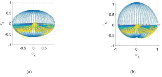
Figure (2a) shows the Barlat Yld2004-18p plastic yield function where the trajectories inside are the gauss point stress recordsin the solid.The geometrical configuration is aL-shapedcantilever beam clamped in one of its borders, whereas in the other border a vertical traction isapplied. Figure (2b) shows the final yield function after the optimization procedure. The yield function has been parameterized by a set of control points (red points) distributed along the yield surface. The initialization of the optimization problem is done with a unit radius sphere.As it can be seen, the excited part is similar to the Barlat yield function. On the contrary, the top part of the optimized yield function did not move because the lab experiments to calibrate the yield did not take into accountthat region. That is the reason why, if the yield function is intended to be well captured everywhere,it is crucial to take a set of experiments which are able to excite the yield function everywhere.

(a) (b)

FIGURE 2.(a) Cantilever beam gauss points stress records for Yld2004-18p. (b) Cantilever beam gauss points stress records

Even though, an optimization problem can be settled in order to find the best candidate, it will require a lot of trial simulations to converge to the local minimum. Moreover, if each is computationally expensive, the global cost of the optimization will be prohibitive.

Another application related to plasticity is to infer the plastic yield function when only the information at certain points is known. Imagine a situation where after computing several homogeneous tests, the plastic yield function is only well calibrated at certain points of the surface but nothing has been said about the rest of the plastic yield. Then, data completion techniques are needed in order to complete the material response under any possible solicitation. The common point of both problematics resides in performing a smart interpolation when the objective function is known just at certain points which are not necessarily uniformly distributed. In what follows we propose a sparse counterpart of the PGD able to proceed in multidimensional settings.

SPARSE-PGD

The main ail of the present section is to develop new strategies with respect to traditional interpolation methods so that fewer points are required to give an overall estimation of the response surface. For the sake of simplicity, but without loss of generality, let’s suppose that a two dimensional objective function, f(x,y) is desired to be approximated. Eq. (2) shows a standard weak form typical from FEM approximation.

ඵ

ݑ

_{(ݔ, ݕ)(݂}

₍

_{ݔ, ݕ}

₎

_{െ ݑ}

₍

_{ݔ, ݕ}

₎

_)݀ݔ݀ݕ

= 0

Nevertheless, the integral that multiplies the test function times the objective function is only known in few points (the ones corresponding to the measurements). Several options can be adopted in this scenario, for instance, the objective function can be first interpolated everywhere and then projected into the basis of the test function. However, the converged solution of this procedure will capture the already interpolated solution in the high dimensional space but in a more compact format. That is the reason why, we will like to first do the projection and then interpolation. Therefore, the test function is constraint to a set of Dirac delta function collocated at the P points at which measures were performed, as shown in eq. (3).

ݑ

(ݔ, ݕ) = ෍ ߜ(ݔ

, ݕ

)

݅=1

(3)

Hence, the integral is transformed into a sum at the collocation points. The next step isto express the approximated function as a set of separated unidimensional functions, like in the classical PGD framework.

ݑ(ݔ, ݕ) = ෍ ܺ

(ݔ)ܻ

(ݕ)

݇=1

(4)

The last step is to provide a basis for each one of the unidimensional modes appearing in equation (4). Several options can be adopted, local linear shape functions, global non-linear shape functions, maximum entropy interpolants, etc. In this particular case, simple Kriging interpolants have been used in order to get relatively smooth solutions, avoiding spurious oscillations characteristic of high order polynomial interpolation:

ܺ

(ݔ) = ෍

ܺ

ܰ

+ ෍ ߣ(ݔ) ൭ܺ

െ ෍

ܺ

ܰ

൱

ܻ

(ݕ) = ෍

ܻ

ܰ

+ ෍ ߣ(ݕ) ൭ܻ

െ ෍

ܻ

ܰ

൱

Combining equations(2-6) a non-linear system of equations is obtained, which is solved using an alternate direction scheme, classical in the PGD framework.

(a) (b) (c)

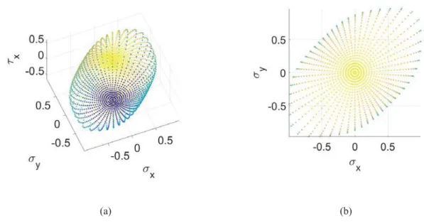
FIGURE 3. (a) Biaxial Barlat Yld2004-18p surface in polar coordinates R (˥˥) for different isotropic hardenings (h). Control

points used in the interpolations (Red). (b) 2D Linear interpolation. (c) Sparse PGD interpolation with simple Kriging interpolants.

Figure (3a) shows a response surface made out of different biaxial Barlat yield functions in polar coordinates for different isotropic hardening levels. The red control points are randomly distributed along the surface. Figure (3b) depicts the interpolated response surface using piecewise linear shape functionsbased on a Delaunay triangularization of the red control points.Figure (3c) represents the interpolated surface based on the same control points but using the sparse PGD algorithm. As it can be seen, the new algorithm takes profit of the separability of the reference solution providing less error than classical linear interpolations.

REFERENCES

1. F. Barlat, H. Aretz et al., “ Linear transformation-based anisotropic yield functions” in International Journal of Plasticity, 2005, vol. 21, pp. 1009-1039.

2. F. Barlat, J.C. Brem et al., “Plane stress yield function for alluminium alloys sheets – Part I : Theory” in

International Journal of Plasticity, 2003, vol. 19, pp. 1297-1319.

3. F. Barlat, D. J. Lege, J.C. Brem, “A six-component yield function for anisotropic materials” inInternational Journal of Plasticity, 1991,vol. 7, pp. 693-712

4. F. Chinesta, P. Ladevèze and E.Cueto, “A Short Review in Model Order Reduction Based on Proper Generalized Decomposition” inArchives of Computational Methods in Engineering, vol. 18, pp. 395-404.

5. E. Onate, S. Idelsohn, O.C. Zienkiewicz, R. L. Taylor, “A Finite Point Method in Computational Mechanics. Applications to convective transport and fluid flow” in International Journal for Numerical Methods in Engineering, 1996,vol. 39, pp. 3839-3866.

6. A. Ammar, B. Mokdad, F. Chinesta, R. Keunings, “A new family of solvers for some classes of multidimensional partial differential equations encountered in kinetic theory modeling of complex fluids. Part II: Transient simulation using space-time separated representation” inJournal of Non-Newtonian Fluid Mechanics, 2007, vol. 144, pp. 98-121.

7. A. Ammar, F. Chinesta, A. Falco, “On the convergence of a greedy rank-one update for a class of linear systems” in

Archives of Computational Methods in Engineering, 2010, vol. 17, pp. 473-486.

8. Q. Meng, Z. Liu, B. E. Borders, “Assessment of regression kriging for spatial interpolation – comparisons of seven GIS interpolation methods” inCartography and Geographic Information Science, 2013.vol. 40, pp. 28-39.