HAL Id: hal-02191402
https://hal-lara.archives-ouvertes.fr/hal-02191402
Submitted on 23 Jul 2019
HAL is a multi-disciplinary open access
archive for the deposit and dissemination of
sci-entific research documents, whether they are
pub-lished or not. The documents may come from
teaching and research institutions in France or
abroad, or from public or private research centers.
L’archive ouverte pluridisciplinaire HAL, est
destinée au dépôt et à la diffusion de documents
scientifiques de niveau recherche, publiés ou non,
émanant des établissements d’enseignement et de
recherche français ou étrangers, des laboratoires
publics ou privés.
Chang Jen-Sin, J.G. Laframboise
To cite this version:
Chang Jen-Sin, J.G. Laframboise. Theory of electrostatic probes in a flowing continuum low-density
plasma. [Rapport de recherche] Note technique CRPE n° 30, Centre de recherches en physique de
l’environnement terrestre et planétaire (CRPE). 1976, 126 p. �hal-02191402�
CENTRE DE RECHERCHE EN PHYSIQUE DE
L'ENVIRONNEMENT TERRESTRE ET PLANETAIRE
NOTE TECHNIQUE CRPE/30
THEORY OF ELECTROSTATIC PROBES IN A
FLOWING CONTINUUM LOW-DENSITY PLASMA
by
JEN-SHIH CHANG and J.G. LAFRAMBOISE
CRPE/PCE
45045 ORLEANS-LA-SOURCE, FRANCE
SEPTEMBRE, 1976 LE DIRECTEUR
SUMMARY
A method has been developed and used to obtain theoretical
prédictions of the current collected from a continuum, incompressible
flowing low charge density plasma by an electrostatic probe having
spherical or cylindrical symmetry. The solutions for the low density
continuum case, i.e. with mean free path « probe radius « Debye
length, are calculated for Reynolds numbers from 0.1 to 100 for
cylinders, 0.1 to 60 for sphères, for charged particle Schmidt
numbers from 0 to lOS, and for scaled probe potentials from -12 to 10
for arbitrary ion-to-electron température ratios. Each current collection resuit has been computed to a relative accuracy of 2%
or better in an average time of approximately 20 minutes on the
CDC 6600 at CNES, including a relative accuracy of 0.4% or better
at stationary conditions compared with the analytic solution. The charge transport, équations are solved using upwind différence methods
developed for time independent situations. Numerical solutions of
the Navier-Stokes équations by other authors are used for the
neutral flow. The electric potential profiles used for the
cylinder are logarithmic, obtained by using the Laplace potential
at the equator of a prolate spheroid, approximated for radii «
major axis. The electric potential profiles used for the sphère are
proportional to r-1, the Laplace potential.
potentials, the effects of the flow increase with potential, and
the usual retarding potential method for température détermination
of électrons leads to large errors, (2) For small potentials, the
effect of the flow is to smooth the "knee" of the probe character-
istics and to render more imprécise the détermination of the
space potential. (3) At a large enough attracting potential, the
linear dependence for probe current from stationary theory is
re.covered as one would expect. (4) The probe surface current
densities become unsymmetrical when flow is increased. (5)
Recirculation in the neutral wake behind the body has larger effects
on downstream than upstream probe surface current density. (6) In
the présence of flow, the prdfiles of net charge density can include several régions of alternating sign downstream of the probe.
Computed charge densities and probe surface current densities
are presented graphically. Computed probe characteristics are presented in graphical and tabular form. A listing is included of
ACKNOWLEDGMENTS
We wish to express our spécial appréciation to K. Kodera
for valuable discussions and comments, and to Dr. L.R.O. Storey
for varieties of assistance too numerous to list.
We are indebted to the C.N.E.S., Toulouse and Bretigny,
to the C.R..P.E., Orleans-La Source, and to York University, Toronto, Canada, for the use of their CDC 7600, CDC 6600, IBM
360 and IBM 370 computers.
Spécial thanks are due to Dr. S.C.R. Dennis (University of
Western Ontario, London, Canada), J.D. Hudson (University of
Sheffield, England), and K. Takami (Tokyo University, Japan)
for providing us with numerical viscous flow data.
We wish to thank the Director of C.R.P.E. for the opportunity
TABLE OF CONTENTS
List of Symbols
1. Introduction 9
2. Statement of the Problem 15
3. Basic Equations and Boundary Conditions 17
3.1 Cylindrical Coordinates 18
3.2 Spherical Coordinates 21
4. Numerical Methods and Calculation Procédure 23
4.1 Time Independent Upwind Différence Methods 24
4.2 Numerical Intégration and Différence Methods 37
4.3 Calculation Procédure 40
5. Results and Discussion for Cylinder in Cross-Flow 43
5.1 Charge Density Profiles 43
5.2 Local Current Density 45
5.3 Total Probe Current 47
5.4 Application to Présence of Magnetic Field 50
6. Results and Discussion for Spherical Probe. 51
6.1 Charge Density Profiles 51
6.2 Local Current Density 52
6.3 Total Probe Current 54
7. Comparison with Experiments and Other Théories 57
7.1 Cylinder in Cross-Flow 59
8. Concluding Remarks
65
Références 68
Tables -
Figures
Appendix A: Application of Theory to Quasi-Neutral Conditions:
y*D-9
Appendix B: Application to Plasma Diagnostic Method
List of Symbols
D diffusion coefficient
e magnitude 'of électron charge
h shape constant
I total collected current for spherical probe; total collected
current per unit length for cylindrical probe.
J local current density
k Boltzmann's constant
K
o (x) modified Bessel function of zéro order t probe length
N number density
R radius
Re Reynolds number based on diameter,
2U CD R p Iv S surface àrea Se Schmidt number, v/D T température U flow velocity V potential
ÀD. Debye length, (e o kT e /eaN oo )* \ mean free path
� mobility
�stream function V kinematic viscosity
Nondimensional Symbols
i=
I/Id, total current , Id = eN^ DSp/Rp
j = JRp/N D, local current
L « major to minor axis ratio of prolate spheroid used to
model cylindrical probe; for relation between L and A see p. 11. n = N/N , number density
Re = 2U
R p Iv, Reynolds number Ra = � 2U
CD R P ID,
diffusion Reynolds number
Se = v/D, Schmidt number u = U/U , flow velocity
cp = eV/kT , potential
e = T/T , température ratio
A = ji/Rpî length of cylindrical probe. For relation between A and L see page 11.
Subscripts a ambipolar b boundary c charged particle d diffusion e électron i ion K itération number k ,2, m grid point o at space potential p probe r radial component z axial component e angular component » at infinité radius
1. INTRODUCTION
A method has been developed and used to calculate the space
charge density profiles near spherically and cylindrically
symmetric electrostatic probes immersed in a flowing low charge density
continuum plasma, and thereby to calculated the current collected
by such probes from the surrounding plasma. A low density
continuum plasma is one in which mean free path « probe radius
« Debye length.
An electrostatic probe is a pièce of conducting material
that is inserted into a plasma on a mechanical support which
provides electrical connection from the probe to external
circuitry (Fig. 1.1). The probe potential is varied, slowly
enough to eliminate transient effects, over a range that
normally includes the plasma potential. The electric current
collected by the probe from the plasma is recorded as a function
of probe potential. The shape of this curve, known as the "probe characteristic", dépends on the composition, the flow velocity and
the thermodynamic state of the plasma, and therefore information about thèse plasma state parameters can often be obtained from one
simple curve. Compared to many other diagnostic tools the probe is
distinguished by the possibility of direct local measurements of
plasma parameters. Thèse facts enable the expérimenter to use plasma
that exist either in the laboratory or in nature. Figure 1.2
shows the general appearance of a probe characteristic. Two
phenomena which appear in figure 1.2, i.e. secondary ionization
caused by accelerated électrons and électron émission from
probe surface due to ion bombardment, are not studied in the
présent work.
Two important examples of low density continuum plasmas exist in nature, that is planetary lower ionosphères and strato-
sphères , and electrostatic probes are frequently carried by
planetary probes or balloons in order to investigate their surround-
ings.
The local disturbances created in the ionosphère or strat-
osphère by the entire planetary probe or balloon can often be
analysed using théories developed for electrostatic probes,
since the vehicle itself constitutes a conducting object immersed
in a plasma; in this case there is no external connection to allow current to drain off, and the planetary probe or balloon will
arrive at an equilibrium or "floating" potential at which it
collects no net current (Fig. 1.2).
Récent developments of flowing afterglow plasmas, flowing
gaseous lasers, diffusion flame plasmas, discharge physics and
atmospheric electricity hâve created a need for probe measurements
in conditions of low charge density (� 108cm"3) and médium neutral pressure (�1 torr) plasma, i.e. under conditions in which the Debye
length may be relatively large but the mean free path is relatively
small. The approximate range of probe conditions in thèse various
flowing plasmas is shown in figure 1.3. Also, in probe
measurements it is always advantageous to use the smallest probe
size consistent with electrical and mechanical constraints, in
order to get minimum
plasma
disturbance and maximum localization of
measurements. In this work, we develop a numerical method to obtain
the probe characteristic for the limit in which ionization is
slight enough that Debye length » probe radius, so that the electric
potential profile surrounding the probe obeys Laplace's équation.
Numerical solutions by other authors are used for the neutral flow.
In order to solve the partial differential équations arising
in this problem, we hâve developed an "upwind différence method" for the time independent case, in order to obtain faster
computation time and stability of calculations (Chapter 4).
In Chapters 5 and 6, we présent results of computations
carried out for cylinders in cross-flow and sphères in flow. We
use the numerical results to demonstrate that the usual retarding
potential method for électron température measurement leads to
serious error in flowing continuum conditions. We also examine the
charge density distributions around sphères and cylinders in the
présence of flow. Then we find that the profiles of net charge
density can include several régions of alternating sign
théories are discussed in Chapt. 7. The application of the
présent work to the limit
R /\Tr*a�
1.1 SUMMARY OF INCOMPRESSIBLE FLOWING CONTINUUM PROBE THEORIES
A summary of probe théories for both sphères and cylinders in incompressible flowing plasmas is shown in figure 1.4. The
présent work is for Debye ratio R /\
= 0 (Chapts. 5 and 6) and oe
(Appendix A), values for which no previous théories exist.
The general theory for probes in flowing plasmas has been first done by Lam (1964). He assumed that under the condition
Xn/R « Re , the neutral flow affects the charge density only in the quasi-neutral
région, since the plasma sheath is much smaller than the neutral flow
boundary layer. He obtained a general expression for flow effects
on current-voltage characteristics. Cléments and Smy (1969)(1970) obtained approximate solutions for sphères and cylinders by comb-
ining the model of Lam with an assumed circular sheath edge
centered downstream of the probe center. Huggins (1974) used the
same model with an approximate thick sheath solution by Keil (1968)
to extend the theory to
R /\ ~
1 for sphères. Hirano (1973)
obtained an approximate solution for cylinders by applying the
model of Lam with his own approximate neutral flow solution at
the front stagnation point. Yastrebov (1972) obtained solutions
for the sphère front stagnation point by using the incompressible nonviscous flow solution for R
/X~^l.
Ail of thèse théories deal primarily with conditions in which the
neutral Reynolds number Re is comparable with the charged particle
diffusion Reynolds number Ra, i.e. the charged particle
Schmidt number
order unity. But the important range of the diffusion Reynolds number is 0 to 104, Le. 0.1 to 102 times larger than the neutral
Reynolds number, in the applications indicated in figure 1.3 for low
density plasmas. Kodera (1975) used the analytical solutions of
Van Dyke (1964, p.159) to estimate the neutral flow for Reynolds numbers 0 to 103 at the front stagnation point. He obtained
solutions for
R /\n � 0, and Ra from 0 to 104.
A large number of références exist on the problem of a
flat-plate probe in a continuum flowing plasma. Thèse hâve been reviewed
CHAPTER II
2. STATEMENT OF THE PROBLEM
In order to define a mathematical model for the plasma, the
following assumptions hâve been made:
1. The plasma consists of two species of charged particles,
one positive and one négative together with neutrals. Far from the probe, the net charge density approaches zéro. Linear
relations between current density and gradients are assumed for both
species. In many expérimental situations, thermal contact
between species is weak enough to allow significant température
différences to exist between them if one of them acts as an
energy source or sink . Therefore, an arbitrary température ratio
is allowed in the theoretical model. In most applications the
électrons hâve the weakest thermal contact with other species-,
2. We assume an unbounded, steady state, constant-property
frozen-chemistry plasma with no magnetic field.
3. The plasma is slightly ionized, so that the mean free
paths between ions or électrons and neutral particles are much
smaller than the meàn free path between ions and électrons.
4. The neutral flow is assumed incompressible.
5. The probe surface is assumed fully charge absorbing.
6. We assume that the Einstein relation � = kT between diffusion coefficent D and mobility jj. is valid for ail charged
constant and T is température.
7r We assume that Debye length
X~ » probe
radius R »
ail
charged particle mean free paths, so that the electric potential
near the probe obeys Laplace's équation.
8. We assume that the diffusion coefficient and mobility
are constant everywhere. This means that the so-called
"cooling effect", (Chapkis and Baum 1971) in which the probe cools
the local plasma, thereby locally changing the diffusion coefficient
and mobility, is not considered in this theory.
9. The plasma is slightly ionized, so that the coupling
3. BASIC EQUATIONS AND BOUNDARY CONDITIONS
According to the above assumptions (Chap. 2), the governing
équations and boundary conditions (Lam 1964) then are:
J - N U - 4 Ni W" Di 7 Ni; v - i = 0 (3.1) J « N U+u, N 7V-D VN;VJ =0 (3.2) ^V,= 0 (3.3) R-R: N. = 0, N = 0, V = V ����� f (3.4)
where N is the number density, V is the potential, R is the radius
and J is the current per unit area. Subscripts i, e, p, »
refer to the ions, electrons, probe surface and infinité radius respectively.
The total ion or électron current I collected by the probe is given by:
I = te JJ* J- dS (3.5)
evaluated over the probe surface S, where the differential area
vector dS is oriented outwardly. We introduce nondimensional
variables as follows; JRp .AN 2UqbRp u eV Ra - D u - u cp = kT eo e e = T eD JL T » �* - kT ' R e P
\7 R p
The governing équations and boundary conditions then reduce to: ciRai j = -2e n + ne ^"^V NV ' J-e = ° (3.7) Vfcp =0 (3.8) r = 1: nt - 0, ne = 0, cp = cp p r-eo:
ni-1, ne-1, cp-O (3.9)
Using équation (3.8) and assuming that the flow is incompressible,
i.e. \v � u = 0, we obtain from équations (3.6) and (3.7).
Ra
2 U'\\In +\\In -\Vcp-\V3 n = 0 (3.11)
From the governing équations (3.8), (3.10) and (3.11), we hâve
an uncoupled situation for n. and n . Also, équation (3.10) is similar to équation (3.11), but with
cp/ei and Ra. replaced by -cp and Ra , respectively. If we solve équation (3.10) for ion density this solution can then be applied to the équation (3.11) for électron
density. Equations (3.10) and (3.11) cannot be solved by analytic
methods because u in thèse équations is obtained from numerical
results by other authors. Their solution by numerical methods is
discussed in Chapter 4.
3.1 CYLINDRICAL COORDINATES
A cylindrical coordinate system (r,0,z) with axis along the center of the cylinder is chosen with 9=0 as the downstream radius.
The fluid motion and electric potential field are assumed to be
two-dimensional and hence independent of the coordinate z. The
fluid motion is described by radial and transverse components of veloclty
(u ,u ) . The velocity components are expressed
in terms of a
dimensionless stream function \|r(r,9) by the équations
Since we want a fine computational grid close to the probe surface
and we also need a large outer boundary radius for computations, we
transform the radial coordinate using the relation s = jjn r, as follows:
os or ' as2 or or
Equation (3.11) then becomes, removing subscripts: Ra exp( s) on
on _ on �g . âS * £ . , ÔÎ £ . â!^. 0 (3 I3ï
2
Us OS + ue oe os as 06 â6
�
îe-r
The appropriate solution of Laplace's équation (3.8) for the
cylindrical case can be obtained from the solution for the equatnrial plane of a prolate
spheroid, approximated for radii « major axis (Moon and Spencer 1961
p. 240, Chang and Laframboise 1975).
For a spheroid of equatorial radius (semi-minor axis) Rp and
half-length (semi-major axis) LRp, with L»l, this potential is:
�p = cp (1 -
jfcnr / £ n2L) (3.14)
dr Zn 2L r
scaled potential
cp /Xn 2L as a parameter in solving (3.13)
for a
cylindrical problem. This is important because it enables us to
treat together ail sufficiently long cylindrical probes. In using
our results to interpret probe measurements, L must be related to
the probe length-to-radius ratio A. Clearly A � 2L; the exact relation between A and L will dépend slightly on e.g. whether the
probe support is insulating or conducting. With this kept in
mind, we assume A = 2L in what follows.
The neutral f low solutions of Takami and Kellar (1969) and
Dennis and Chang (1970) were used to provide
(u , ufi) in (3.13). Takami and Kellar (1969) solved thé Navier-Stokes équations
numerically for steady two-dimensional viscous flow of an incomp-
ressible fluid past a circular cylinder for Reynolds numbers from
1 to 60 (Fig. 3.1). Dennis and Chang (1970) hâve extended the work of Takami-Kellar to Reynolds numbers from 0.1 to 100 (Fig. 3.2).
The numerical values of
(u , u ) of Takami-
Kellar and Dennis-Chang
were used during the numerical solution (Ch. 4) of équation
(3.13). Thèse authors hâve not provided sufficient information to
permit us to evaluate the effects of errors in their solutions on
our results. However, for Reynolds numbers of 7, 20 and 40,
neutral flow solutions from both of thèse papers are available
(Figs: 3.1, 3.2). For Re = 40, we hâve calculated total probe
current using both flow solutions. In this calculatiqn we also
used the values Se = 10 and çp =
0. The two results agreed to within
2%, even though grids of 40x40 and 60x60 points were used
3.2 SPHERICAL COORDINATES
A spherical polar coordinate system (r,9,§) with the origin at the center of the sphère is chosen with 0=0 as the downstream
radius. Both the fluid motion and electric potential field are
axially symmetric and hence independent of the azimuthal coordinate
Ç. The fluid motion is described by radial and transverse components
of velocity
(u ,u ) in a plane through the axis of symmetry.
The
velocity components are
Ur
=
1-2
sine Ô-9 '
U9
=
r sin e - Õr
(3.16)
Equation (3.10) then becomes, after removing subscripts'
2
Us OS ese'
os ds de ae
aS2 bS be2
ae
(3.17)
Boundary conditions are the same as in équations (3.9).
The appropriate solution of Laplace's équation (3.8) is'
*- £
�
o?=-r £
(3.18)
The neutral flow solutions of Dennis and Hudson (1973) were used
in (3.17). Dennis and Hudson (1973) solved the Navier-Stokes équations numerically for steady flow past a sphère for Reynolds
numbers from 0.1 to 60 (Fig. 3.3). The numerical values of
(u , ufl) of Dennis and Hudson were used during the numerical solution
4. NUMERICAL METHODS AND CALCULATION PROCEDURE
Accordingto Chapter 3, we need to solve the elliptic partial
differential équations (3.13) and (3.17) by numerical methods.
In this chapter, we présent new "upwind différence" methods
(Sec. 4.1) developed for time-independent situations in order
to obtain faster computation time and stability of calculations.
The local current fluxes are calculated by an extrapolation
method (Sec. 4.2) and the total currents are calculated by Simpson's
intégration rule with Richardson's extrapolation method (McCormick
4.1 TIME INDEPENDENT UPWIND DIFFERENCE METHODS
The usual methods for numerically solving elliptic partial
differential équations with variable coefficients are the
Successive Over-Relaxation Method, the Alternating Direction
Implicit Method and the Quasi-Linearization Method (Smith 1965).
Each method involves writing � and
-7-5- in finite-difference
approximation form and solving for n approximately using the itérative
method called relaxation (Smith 1965), in which the values of n at
points in the computational grid are successively replaced by linear
combinations of the surrounding values.
dsn The usual finite-difference approximation of -r-g- is
2 n + n m-1 - 2n UX-2 AX2
+ ° (^) (4.1)
The usual expressions for the différence
� are as follows.
(i) forward difference:leads always to stable solutions
(ii) backward différence; always leads to stable solutions
(iii) centered difference:leads to a solution stable only for
small enough e (Fukuda 1969)
dn Vl2LcVl
where Ax =
x m xm-i = xMi- 1 - XM
The usual way for solving elliptic partial differential
équations uses centered différences, because the accuracy is higher
than for the other two methods. However, numerical instabilities
occur in this centered différence method because of round off error
and the "hereditary error" (Fukuda 1969) for large Ax. The
backward and forward différence methods always lead to a stable
solution for any Ax (Fukuda 1969).
We suppose that the (s, 9) space is divided into a grid of LxM points separated by distance incréments h. Then we can write the
coordinate distances as s = jîh and 9 = mh where m = 0,1,2,...,M
and jfc = 0,1,2,...,L. Thus any point on the grid is uniquely identified by the indices ( £ ,m). A portion of such a grid space
is shown in Fig. 4.1.
Next we write the partial differential équation in finite-
difference form. We now consider the problem of solving the
équation for n.. The substitution procédure for n. is
determined by substituting the chosen différence expressions into
the given équation and solving the resuit for
n. X,m
in terms of the
into two classes: (1) simultaneous relaxation, and (2) successive
relaxation.
Since relaxation is an itérative procédure, some method is
needed to identify the order of approximation. We thus label n
with the superscript K to indicate the Kth guess n . If the method
is convergent, n should approach the true solution n at ail points as K CD. In the simultaneous relaxation, the (K+ l)th guess
K+l K K
can then be computed according to (Smith 1965) n.
X,m = n, 1 m + oR. a, m , where
R, X,ni is the residual,
which is equal to the différence between the resuit
for n, In terms of surroundLng values, and the previous value n� , and �y is a constant which dépends on the finite-difference form and the constants in
the differential équation. Then in the simultaneous relaxation, the
entire new field
n. is calculated using residuals computed
from
the old field."
However, it is clear that once a new guess has been made at
a given point, the new values can be used to modify the residuals at the surrounding points. Thus, the residuals can be computed sequentially starting from grid point (1.1) and working to the
right along the grid to point (L-1,1), then skipping to the second
interior row of points and working from point (1,2), to( £ ,-l, 2), etc.,
as shown in fig. 4.1. This scheme is called successive relaxation.
In this case the residual at (t,m) is computed using two old guesses
and two new guesses at surrounding points ( £ + l,m), ( £ -l,m), (1, mfl) and (t,m-1) as shown in fig. 4.1. In this method, the
relaxation (Smith 1965).
Upwind différence methods were intrcduced by Leith (1965) for
solving time dépendent differential équations. The results show
that the solutions are well stabilized during the calculations.
We hâve developed upwind methods for our governing équations with
convection term for the time-independent case, in order to obtain
faster computation time and stability of calculations. In the
partial differential équation as follows
calculation instabilities occur when Ra is relatively large in
ail centered différence methods. This is believed to be caused
by loss of diagonal dominance(Greenspan 1975, p. 218).
In our équation (4.5), u sometLmes contains a wake (région of recir- culation) behind the probe (Figs.3.1-3.3), and this might also be
an important source of instability in calculations by other authors.
The idea of upwind différence methods is based on the observation
that in a convective situation, physical information is transported
from the upwind direction, so that some combination of numerically
stable forward différences may give the most use fui approximation
of the (u-\vn) term. Also, we shall see that the methods are very
4.1.1 LOWER ORDER METHOD
The grid structure of the method is shown in figure 4.2 with the local wind vector u at the central point (t,m). Hère we use
rectangular coordinates x and y. In figure 4.2, the wind direction
has been chosen such that u � 0 and u � 0. The (u \\In) term in (4.5) can be approximated by either of the following backward
différence expressions:
or
u.NVn = g (n n (n n
(4.6b)
We first consider the purely convective situation in which no
diffusion or potential gradients exist, and (4.5) reduces to u«\vn=0.
We wish the information to be transported only from the upwind
direction, so we require that our substitution process hâve the
following properties: If u - x 0 then n n m- 1 (4.7) If uy m 0 then n, = n. ,
The following linear combinations of (4.6a) with (4.6b) hâve thèse properties.
UX + 02UY
If u � u thenu.\vn = � ^ �- (4.8)
x y """
If
il,
�
Uy
then u«\vn
lt:,y
ÙS.
(4.9)
Ujj/ax
+ uv/Ay
The fact that (4.8) and (4.9) satisfy the conditions (4.7) can
be readily verified by assuming u � \vn = 0, substituting (4.8) and
(4.9) into this relation, and solving for n..
Thèse relations also hâve another important feature, which we
can see as follows.
We define q = J . , and we then obtain: (i) if u �u (q�l)
UxuY
x
y
then u-\vn 1 ; [n, _+ (q-l)n.. - qn...] (4.10) (ii) Ifux�uy (q�l) luxlIf we again assume u-\Vn=0 and équations (4.10) and (4.11) for n, we obtain if q � 1, then n. = (1 - q) n.. + qn, .. (4.10') if q� 1, then n. = (1_1) n, 1 + q 1 (4.11') i.e. if q � 1, n. A, m
becomes just the value of n at the upstream
point A in figure 4.2, as determined by linear interpolation
between the values
n. -
and
n... If q � 1, n. "
then
becomes the value at the corresponding upstream point on the
Similar relations can be obtained easily for the other three
cases; (a) if u � 0,
u
� 0, we replace nn 1 , n.. , and n
by Vl,m' nnil and n. l, respectively, (b) if u � 0, u � 0 we replace thèse values
by n, . , n. ,
and
n, ,, respectively (c) if u � 0, u � 0, we replace thèse same values by
n. ,
n. -
and
n, - , respectively.
We therefore hâve an algorithm
which is always in accord with the essential physics of our
situation, i.e. in the purely convective limit it causes information
always to be transferred in the downstream direction along stream-
lines. A similar method by Carlson (1967 p. 240) exists for
4.1.2 HIGHER ORDER METHOD
The interprétation of (4.10') and (4.11') in terms of linear interpolations suggests that a more accurate method can be obtained
by simply replacing thèse interpolations by higher-order ones,
involving more than two collinear points (figs. 42,4.3). For the
sake of illustration, we consider this time the case
when ux �0,
il, � 0 and q�l. We first fit the density values n n. ,,
and n. -
. with a parabola as follows.
n-n
t,mf- eA., §+A2 §2, where = (x-x £ )/Ax.
We then hâve: and : Solving, we obtain: AI - Vl.mt-r nA-l,mfl 2 A nX-l,mfl+nx+l,mfl" 2n (4,13) and nk, =
n^ ^^A,^ q'+Ag q 12 where q7 - 1/q
Next, we fit
n.. , n , ., and n
with another parabola.
a ' "l+2,nn-l + n ,t,mrl 2n
�2 -
Again when u-\vn=0, we recover, as we should, the following:
lf q'- - 0 then nk, = n^^ and n^ - n^, if q' = 1 then kl = n^^ and n^ = n^^ .
The best way of also satisf.ying. the conditions corresponding to (4.10') and (4.11') is: n nk2 + (nkl- nk2)(1 - q") (4.15) Therefore, we obtain n (g 2 -1) [n 1 (3q2 - 2q' - 2) + n (1 - ,'),' ' + V2,*!'"! + VcVii-n(1-3q'" + 4q (4.16a)
and
-
u'\vn = - (n m - es) where as is the right hand side of (4.16a).y
..t.,m
For q �1, from the same mathematical process, we obtain
nA,m " (q-l) 2 [ ( 2 ( + Vi.-*2««+! EVi.»i(1-3'B + 4q) (4.16b) and u-\vn = -»�*� (n - B4) where B4 is the right hand side of (4.16b).
In spécial cases where.
n. A, m
is near an edge or a corner,
we use n.
m é. instead of équation (4.16a) or (4.16b).
Similar relations can be obtained easily for the other three
cases: (a)
u � 0, u �0 (b) ux � 0, u � 0 and (c) ux � 0, uy � 0.
Therefore, the numerical method in our case is to express the
^n, �57cp'\vn terms by central différences and u -NjTn by the higher order upwind différence' form and to use successive relaxation to solve the
charge transport équation (3.13) or (3.17) for n (we call this
method "upwind différence method" in later chapters). In applying
thèse methods to (3.13) and (3.17), x and y are replaced by e and
s, respectively, and u and uy are replaced by u.
and
4.1.3 ACCURACY OF NUMERICAL METHOD
In order to estimate the accuracy in our numerical methods,
we numerically solved two problems which hâve known analytic solutions. Thèse problems involve the usual convection-diffusion
équation:
URpln
£ n
where
we hâve assumed
uniform
flow
in the
x direction.
An analytic
solution
of (4.17)
(Dennis
et al 1973)
for
spherical
coordinates
is
where
Ra =UR
/D,r
= J xa +
y3 +
za and n
1 when
r » (point
source
in uniform
flow).
An analytic
solution
for
cylindrical
coordinates
is (Dennis
et al 1968).
n - 1 + G, exp [ Sp cos e ] K Ea r
(4.19)
where
K
o
(w)
is the
modified
Bessel
function
of zéro
order,
and
r - J x 8 +
y8 (line
source
in uniform
flow). For example
in
cylindrical
coordinates,
if we solve
équation
(4.17)
numerically
with
boundary
conditions
obtained
using
numerical
values
of équation
(4.19),
we can obtain
the
relative
error
in our numerical
methods.
We solve
(4.18)
and (4.19)
numerically
in the
domain
(r
�
r
�
r,,
0
�
e
�
ir).
��
"'"
�
.
r = r : n, =
1 + 2exp
[=
cos 9
] K (-2 )
r -
b
nb .9m 1 +
2exp [Ra 2 rb
cos e m
K 0
( R?)
with similar
boundary
conditions
from
(4.18). In either
case
we
also hâve:
9
9 = 180° :
on
0
where we
choose
Ca
= 2, Ra = 10,
r = 1,
rb
= 25 to define
our
two test
problems.
With this
choice
the
variation
in each
solution
over
the chosen
domain
is of the same
order
as the solution
itself.
The values
which
the
analytic
solutions then
hâve
at r = 1, 9 =0° and
180°
are 2.181
and 1.0 respectively
for
the cylinder,
3 and 10
respectively
for the sphère.
The uniform
flow
in the (r,9)
coordinates
is
u. =-sin 9 ,
u
cos 0 .
r
m
We again
transform
the radial
coordinate
using
the relation
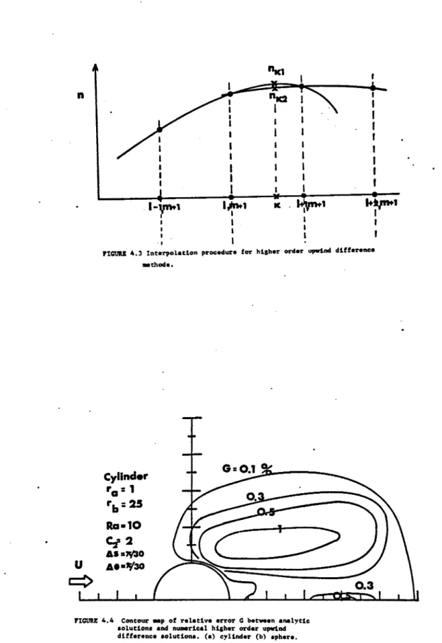
s = ln r. In figure
4.4,
we show
the
relative
error
between
analytic
solutions
and numerical
solutions
for
a) cylindrical
coordinates
b) spherical
coordinates,for
A9 =
As «
TT/30.
From
figure
4.4,
we find
the
maximum
error
at 9=0° and e = 40° -500.
We also find
that
the
error
at the
détermination
of local
current
fluxes
to the inner
boundary
r= 1 is smaller
than
0.1%
in both
spherical
and cylindrical
cases. The reason
for the larger
errors
downstream
than upstream
is the larger
density
gradients in
thèse
analytical solutions downstream. The maximum relative
error of both spherical and cylindrical cases is shown as a function
of 6e in figure 4.5 (where A0 = As for each calculation,
ùe- E) t- 9... and As = Xnr - Xnr . ). From the slopes of the lines in figure
m m-1
4.5, we hâve obtained graphical estimâtes of the actual order of
the methods. For the sphère, we obtained 0(Ó,91.06) for the lower
order method and 0(Ó'e1.48) for the higher order method. For the
cylinder we obtain 0(6g1.22)for the lower order method and 0(Ó'e1.57)
for the higher order method. For the lower order method, we can say the order of the method is slightly better than 1, but for the
higher order method the order of the method is about 1.5. The
computation time on the CDC 6600 computer by our numerical
methods is shown as a function of the number of grid points in
figure 4.6. The computation time at 30x30 grid points is less
than 200 sec and 140 sec by our numerical method with the upwind higher order différence and the lower order différence, respectively.
Itérative times for the sphère and the cylinder were approximately 1.6
iterations/sec and 3.1 iterations/sec using the higher-order method,
and the itération was stopped in the condition
£ ' |n. A, m - n. A, m1 I £ l0"4.
4.2 NUMERICAL INTEGRATION AND DIFFERENCE METHODS
4.2.1 LOCAL CURRENT DENSITY
The local current density from équations (3.6) and (3.7)
is defined as
J
dr 'r=l ds dr s=0 ds �s=0 (4.20)
In order to obtain a second order différence approximation for
équation (4.20) we fit n, , n_ , and n3 using a parabola as follows n » As s2 + A4 + Ag n l,m = As
= 0 from boundary condition, at probe surface (Eq. 3.4)
n2 m " A3(ûs)3 + M^s) n3,m = 4As(AsOa + 2A4(ûs) :. j = ddn L-o - A4 + 0(6s2) = ^C ^^ + 0(6s2) (4.21)
Similarly, we fit a parabola through
n. 1 ,m n3 and ns to obtain immédiate ly .i-sU- 4n 3,m - "5'm + 0[(26s)2J (4.22)
Equations (4.21) and (4.22) hâve an error of 0(ass) and 0[(2As)8],
respectively. Therefore we may use the Richardson extrapolation
method (McCormick and Salvador! 1964) to obtain a more accurate
value of the local current density. If
approximate expressions for j given
in (4.21) and (4.22), respectively,
then the Richardson extrapolation method yields,
to second order:
j (4j,
ja) /3
=
32n
2,m
-12n
3,m
n S,m
(4.23)
4.2.2 TOTAL CURRENT
The total current for the sphère and current per unit length
for the cylinder are from Chapter 3, Eq. (3.5) as follows:
i"%rn j(6)sine de (sphère) 0 (4.24) . i 2TT 0 217 j(8)de (cylinder)
In order to obtain the most accurate possible value of i, we
used intégration by Simpson's rule with intervais 68 and 26e.
We then carried out Richardson extrapolation on the results obtained in
4.3 CALCULATION PROCEDURE
The block diagram of a calculation is shown in Fig. 4.7.
The charge transport équations (3.13) and (3.17) are solved using the upwind différence methods which we hâve developed in Sec. 4.1. Boundary conditions are from Eqs. (3.9), (4.18) and (4.19) as
follows:
s = 0: n 1 ,m
=0 (from kinetic theory, Lam 1964)
9 - 0° and 180° : §| - 0 (from symmetry)
s = s, = Anr, : n = 1 - (1 - n �r exp C-T^V r ) (l - cos 8 ) (cylinder)
where we hâve used Eq. (4.19) with the approximation:
K(x) a
( 1) k exp(-x) for large x (Dennis et al 1968). The
boundary conditions at s = s, are from (4.18) and (4.19), which we
assume to give the ratio of the two values
n.. and n (Dennis et al 1968, 1973). This procédure is based on the fact that at large radii, the disturbance in number density due to the probe
can be expected to approach that of a sink (négative source) in a uniform flow. Thèse boundary conditions are solved together with
the charge transport équation for each itération in our calculations.
convergence was attained. This décision was made by requiring
In order to achieve the fastest possible convergence the successive
relaxation was done in a generally upstream to downstream order
during each itération. The calculation procédure for local currents
and total currents was checked by trying several values of the grid
intervais AS and As, and several positions of the outer boundary
r, . The values of 68, As and
r, which we used for calculation of
densities, local currents and total currents are shown in Table I.
One more check of the calculation procédure involves the limit in
which Ra (=Sc x Re) is small. In this condition, the numerical
values of total currents and local currents are in good agreement
with the analytical values from the stationary(no-flow)
theory (Appendix B).
Each total and local current collection resuit has been computed
to a relative accuracy of 2% and 5% or better, respectively, in an
average time of approximately 20 minutes on the CDC 6600. In the
spherical case the calculations yielded a relative accuracy of 0.4% or
better in comparison to the analytical solution at stationary
conditions. In flowing conditions thèse accuracies refer only
to the solution of the charge transport équation, and not to the
accuracy of the numerical Navier-Stokes solutions used as input to
the calculations. The accuracy of the latter has been discussed
in Sec. 6.3. In the cylindrical case the results cannot be compared with the
5. RESULTS AND DISCUSSIONS FOR CYLINDER IN CROSS-FLOW
5.1 CHARGE DENSITY PROFILES
Numerical results for charge density contours are shown in
Fig. 5.1 using the solutions of Eqs. (3.12) to (3.151. The effect
of the neutral wake (recirculation région, Figs. 3.1, 3.2) is
shown in Fig. 5.la for a cylinder at space potential with charged-
particle Schmidt number Se slO2. The neutral wake for the cylinder in
cross flow occurs for Re s (Takami et al 1969). Figure 5.la
shows that for a flow with wake (Re = 20), the charge density is
larger in the rear stagnation région than in the case of flow without
a wake (Re=0.4 in Figure 5.1a). The reason is that in the case
with wake, the recirculation of the neutral flow brings charge
to the rear stagnation région.
The effect of charged particle Schmidt number is shown in
Fig. 5.1b for Reynolds number 40. We see that the effect of the
wake in the rear stagnation région increases as the Schmidt number
increases. The effects of surface potential on flow with wake and
flow without wake are shown in Fig. 5.1c (Re=40,
Se =1) and 5.1d
(Re - 0.4,
Se - 102) for both attracting potential (çp le tnA = 4) and retarding potential
(cp p le
jfcnA=-4). For the attracting
potential, the effect of the potential tends to symmetrize the charge
density profile around the body for both flow with wake and flow
If we only hâve two species (ions and électrons) in a plasma, we can numerically subtract density profiles between ions and électrons. We may thereby find the net charge density profile
(n. - n ) for a cylindrical probe.
Usually the diffusion Reynolds number for ions is much larger
than that for électrons. Therefore, we can numerically subtract
density profiles between two différent values of Ra for the same
Reynolds number. The general appearance of some typical net charge
density profiles is shown in Fig. (5.2): (a) for a stationary
case (b) for flow without wake, (c) and (d) for flow with wake.
Figure (5.2) shows that in the présence of flow, the net charge
density profiles can include several régions of alternating sign
downstream of the body. In the case when a wake is présent, thèse
net charge density profiles show more complicated dependence on the Reynolds number and the ion or électron Schmidt number. This
phenomenon may be a very important problem in interactions between
an antenna, electrostatic probe or mass spectrometer and a balloon or planetary probe. The measured plasma parameters can be affected by thèse several régions of alternating sign of the net charged
5.2 LOCAL CURRENT DENSITY
Numerical results for ion or électron local current density j
at the probe surface are shown as functionsof angle 9, where we define 0=0 at the rear stagnation point, in Fig. 5.3 for various
surface potentials, (a) and (b) for Re = 0.1, Sc = 1d3 and 104
respectively, (c) for Re = l,
Sccm icp, (d) and (e) for Re = 10,
Se =10 and 108 respectively, (f) for Re=40, Se =10, (g) and
(h) for Re=100,
Se =0.1 and 10 respectively. Figure 5.3 shows that for flows without a wake (Fig. 5.3(a) - (c», the effect of the
attracting surface potential is to symmetrize the local current
collection and of the retarding surface potential is to unsymmetrize
it. For flows with a wake (Fig. 5.3(d) - (h)), we observe large
current collections at the rear stagnation région. The effect of
the attracting surface potential in thèse cases is to symmetrize
the current collection at large potentials, and also to increase the
asymmetry of the collection at small potentials.
Figure 5.4 shows the influence of the Reynolds number on the
local current angle dependence for
Se = 1, cp /e in A= 0 (a), 4
(b), -2 (c) and for Se - 103 , rn le ln A- 0 (d), 4 (e), -2 (f).
Figures 5.4 (a) - (f) show more clearly the effect of the wake on
the local current collection. As noted earlier (Sec. 3) a wake
exists for the cylinder when Re � 7. We find that the minimum
point of the local current is always close to the flow séparation
potential is changed.
The local currents are shown as functions of the angle in
Fig. 5.5 for various charged particle Schmidt numbers, for Re = 0.4
(a)
cp p le InA-0, (b) 4, (c) -2, and for Re-20, (d cp. p le tnA
= 0, (e) 4 and (f)-2. Figure 5.5 shows that the effect of the
charged-particle Schmidt number on the local current is larger in
the front stagnation région than in the rear stagnation région.
The above numerical values of the local current density can
be used to estimate ion collection by a mass spectrometer orifice
électrode located in a blunt surface under continuum conditions, for
instance in rocket or balloon measurements up to the D-region, in
5.3 TOTAL PROBE CURRENT
The numerical results for the ion or électron currents per
unit length are shown as functions of the charged particle
Schmidt number in Fig. 5.6 for various scaled surface potentials
cp p le An A at Reynolds
number Re = 40. Figure 5.6 shows that for
retarding potentials
(cp /e
in A� 0), the effect of charged
particle Schmidt number increases with the potential. For large
enough attracting potentials, the currents become only slightly
affected by the charged particle Schmidt number.
Figure 5.7 shows the ion or électron currents per unit length
for various scaled probe potentials at
Se = 100. Figure 5.7 shows that the effect of the flow increases with retarding surface
potentials and decreases with increasing attracting surface
potential. Also, in thèse two figures there is a slight decrease
of current as either Re or
Se c increases, for larger values of attracting surface potentials
(cp p le
in A ^ 6 in both Figs. 5.6
and 5.7).
Figure 5.8 shows logarithmic current-potential characteristics
for various charged particle Schmidt numbers for (a) Re=2,
(b) Re=7, (c) Re = 10, (d) Re = 20 and (e) Re = 100. Figure 5.9 shows
similar characteristics for various Re at Se = 103. Tn c
comparison with the usual exponential dependence from
1926; not shown), we see that misuse of the usual retarding
potential method for the température détermination would lead to
increasing T
overestimates as the flow effects increase(See
also Sec.6.3). Aise
we observe that the effect of the flow is to smooth the "knee" of
the probe characteristics and to render more imprécise the déterm- ination of the space potential.
Logarithmic current-potential characteristics are shown in
Fig. 5.10 for various Reynolds numbers at a diffusion Reynolds
number of 103. Figure 5.10 shows that the model developed by Lam
(1964) (Sec. 1.1) cannot be applied to a.low density plasma
(XD » R p),
for the currents hâve a large dependence on Re even
if Ra is constant. The previous work (Hoult 1965) which extended
Lam's model to the low density plasma case should be reconsidered.
Figures 5.11 and 5.12 show currents vs probe potential for
various charged particle Schmidt numbers at Reynolds number 0.4,
and for various Re at Se
c = 10 respectively. At a large enough
attracting potential, Figs. 5.11 and 5.12 show that the linear
dependence
I9cp
from stationary theory (Appendix B) is recovered.
This point is important for the détermination of the électron or
ion température (Appendix B).
a function of the Reynolds number in Fig. 5.13 for various
charged particle Schmidt tunbers, and as a function of the charged
particle Schmidt number in Fig. 5.14 for various Reynolds numbers.
Figures 5.13 and 5.14 show that the effects of flow on nondimensional
current at space potential increase rapidly as Re and Se
increase.
Computed values of probe current are presented in tabular
form in Table II. As we discussed in Chap . 3, the above solutions
for total current, local current density and density contour maps
can be applied to both ions and électrons, but with cp ICiLnA and
Rai for ions replaced by-m ILnh and Ra , respectively, for
5.4 APPLICATION TO PRESENCE OF MAGNETIC FIELD
An important application of the présent results is to a cylindrical probe with its axis parallel to an imposed magnetic
field (Fig. 5.15). We can use unchangedthe results described in
this chapter except that D. and D are replaced by
D. and D ,
respectively, where we again assume that the neutral flow is not
affected by the magnetic field, i.e. we hâve a slightly ionized
plasma, and D is the diffusion coefficient perpendicular to the
magnetic field, D
= D/[l+(u3gT )2] ,(Bohm et al, 1949). Hère uju = eB/m is the cyclotron angular frequency, and
T B is the mean time between collisions with neutrals. The usual Reynolds number is then replaced
by a magnéto - diffusion Reynolds number which is defined as:
2U R
6. RESULTS AND DISCUSSION FOR SPHERE
6.1 CHARGE DENSITY PROFILES
Numerical results for charge density contours are shown in
Fig. 6.1 for charged particle Schmidt numbers of 0, 1, and 10
at Re=5, where the solution for
Se c = 0 is just the diffusion
profile n=l- 1/r. Figure 6.1 shows that the charge density
around the sphère becomes unsymmetrical when the charged particle
Schmidt number increases. The effect of a wake on the charge
density distribution is shown in Fig. 6.2. Figure 6.2 shows that
for the flow with wake (Re = 40), the same phenomenon as in the
case of cylinder in cross-flow (Fig. 5.1) occurs in the rear stagnation région. In both cases this concentration of charge
behind the body occurs at larger values of Se .
Effects of surface potential on charge density profiles are
shown in Fig. 6.3 at Re = 5,
Se c =1
for the surface potentials
cpp/e- -4, 0, and 4. Figure
6.3 shows that the effect of an
attracting potential is to symmetrize the charge density profile
around the body. For retarding potentials, the effect of the
potential is to unsymmetrize the charge density profile. Figure 6.4
shows density-angle dependence for two différent distances from
the probe surface, (a) r = 4.22 (b) r = 1.1275, at Re = 5, Se =1. From Fig. 6.4, we see again that the effect of surface potential
changes is to symmetrize or desymmetrize the charge density
6.2 LOCAL CURRENT DENSITY
Numerical results for the ion or électron local current
density at the probe surface are shown as a function of the angle 9
in Fig. 6.5 for various surface potentials, (a) for Re = 20, Se =1 (b) for Re = 60,
Se =1. Figure 6.5a shows that for flow without a wake, the effect of the attracting surface potential is to
symmetrize the current collection and the effect of the retarding
surface potential is to unsymmetrize the current. The corresponding
diagrams for the cylinder are Figs 5.3(a) - (d). For the flow with
wake (Fig. 6.5b), we observe a wake collection effect in the rear
stagnation région as in the case of the cylinder in cross-flow
(Fig. 5.3(e) - (h)). The effect of attracting surface potential
(Fig. 6.5) in the wake is not to symmetrize the current collection,
but to increase the asymmetry of the collection as in the case of the
cylinder in cross-flow (Fig. 5.3). Figure 6.6 shows the influence
of the Reynolds number on the local current angle dependence for (a)
cp /e = 0, (b) 2 and (c) -4 at Se =10a. In Fig. 6.6, we show the stationary solution (Eq. BU together with the solutions
for nonzero Reynolds numbers. Figure 6.6 shows that in the front
stagnation région, the local currents are larger than the stationary
value. In the rear stagnation région, the local current is smaller
than the stationary value in the flow without wake and sometimes is larger in flow with wake.
The local currents are shown as functions of the angle in Fig.6.7
cp
p le = 0, (b) çp p le = 2
and (c) cp
p le = -2.
Figure 6.7 shows that
the wake effects increase with the charged particle Schmidt