HAL Id: hal-00606226
https://hal.archives-ouvertes.fr/hal-00606226
Submitted on 5 Jul 2011
HAL is a multi-disciplinary open access
archive for the deposit and dissemination of
sci-entific research documents, whether they are
pub-lished or not. The documents may come from
teaching and research institutions in France or
abroad, or from public or private research centers.
L’archive ouverte pluridisciplinaire HAL, est
destinée au dépôt et à la diffusion de documents
scientifiques de niveau recherche, publiés ou non,
émanant des établissements d’enseignement et de
recherche français ou étrangers, des laboratoires
publics ou privés.
Integration of omics data to investigate common
intervals
Sébastien Angibaud, Philippe Bordron, Damien Eveillard, Guillaume Fertin,
Irena Rusu
To cite this version:
Sébastien Angibaud, Philippe Bordron, Damien Eveillard, Guillaume Fertin, Irena Rusu. Integration
of omics data to investigate common intervals. 1st International Conference on Bioscience,
Biochem-istry and Bioinformatics (ICBBB 2011), 2011, Singapore, Singapore. pp.101-105. �hal-00606226�
Integration of omics data to investigate common intervals
Sébastien Angibaud, Philippe Bordron, Damien Eveillard, Guillaume Fertin, Irena Rusu
Computational Biology group (ComBi)
Laboratoire d'Informatique de Nantes-Atlantique (LINA), UMR CNRS 6241, Université de Nantes, 2 rue de la Houssinière, 44322 Nantes Cedex 3, France
{sebastien.angibaud, philippe.bordron, damien.eveillard, guillaume.fertin, irena.rusu}@univ-nantes.fr
Abstract—During the last decade, we witnessed the huge
impact of the comparative genomics for understanding genomes (from the genome organization to their annotation). However, those genomic approaches quickly reach their limits when one looks at investigating the functional properties of genes in the wide genome context. Such limitation may be overcome thanks to recent high-throughput experimental progresses like those obtained via metabolic and co-expression studies, that produce so-called omics data. Therefore, integrating those data and state-of-the-art computational genomic comparison is a natural evolution. This paper achieves such an integration and proposes a heuristic algorithm IISCS that incorporates omics knowledge into the IILCS heuristic, already known as accurate to compare genomes. When applied on bacteria, one emphasize large functional units composed of several operons.
Keywords-comparative genomics; integrative approach; operons prediction
I. INTRODUCTION
During the last decade, comparative genomics provided several computational tools to understand genomes. In particular they give us the opportunity to investigate genome organization that leads us to annotate genes based of their relative location into conserved genomic areas during the evolution of two species. Finding those sets of conserved genes implies the use of a dedicated measure. Common intervals, as computed by the IILCS heuristic, is appropriated to compare bacterial circular genomes [1]. Indeed, a common interval, as illustrated in Figure 1(a), is defined as a set of genes that are located together inside both genomes, not necessarily in the same order and without taking gene orientations into account. Common intervals correspond to conserved areas (i.e. areas with the same genes content) inside which some rearrangements have occurred during the evolution of both species. However, investigating the functional meanings of a genomic comparison remains a difficult task (mainly due to the large number of conserved organizations with no function to rely on). In addition, when applied on the operon predictions at wide-genome information, one must notice that the use of intergenic distance only is not sufficient [2], which leads to investigate techniques that combine omics data to improve the prediction accuracy.
Following a similar philosophy the use of omics data combination, we propose herein to extent the common interval computation with an estimation of their biological
interests by using metabolic or microarray data. Our goal is thus dual. First, we aim at filtering the most relevant common intervals in a context other than genomic only. Second, we consider merging heterogeneous knowledge with a genomic information, which represents one of the key question in integrative genomics. Every step of the method will be illustrated by a concrete biological case, based on the comparison between two bacterial species: Escherichia coli and Vibrio cholerae.
As a preliminary step, the paper will start (Sec II) with a sketch of the common interval computation, which considers, in our process, only genes that are in both genomes. Thus, a gene that has been lost in one of the two genomes during the evolutionary process, or a gene that has been duplicated after the speciation (in-paralogous gene) is not taken into account in the computation process. This technique implies that common intervals can contain a gene that has appeared after the speciation. To illustrate such a common interval, Figure 1(b) gives an example where both genomes do not have the same gene content. As a natural refinement, we will then propose an heuristic for integrating the obtained common intervals with microbial omics data at disposal. As a major contribution, such an integration rises the accuracy of the common intervals which is emphasized by comparing and discussing (Sec. III) our results with known bacterial operons.
II. MATERIAL AND METHOD
A. Genomes investigated
Our biological benchmark is composed of two genomes of proteobacteria : Escherichia coli K12 MG1655 (one chromosome, NCBI id : NC_000913) and Vibrio cholerae 01 biovar eltor str. N16961 (two chromosomes, NCBI id: NC_002505 & NC_002506). In order to benefit from large knowledge on the genome of Escherichia coli, we compared
E. coli with each of the two other chromosomes. B. Computation of common intervals
The comparison between two given genomes, using the common interval measure is implemented in a software called Match&Watch [1]. This program is available on request. It provides a GUI that controls the processes described below, and an automatic graphical representation of common intervals.
Homologies detection: The first step of the method
Inparanoid software [3] (step 1), which clusters ortholog and inparalog genes based on a Blastp. Then, we tag the homologous genes with a similar label according to the clusters (step 2). This step does not take into account separation of orthologs and inparalogs given by Inparanoid.
Matching choice: When genomes contain duplicates, we
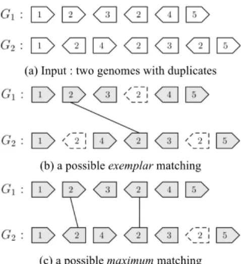
cannot directly compute the number of common intervals, because this measure is defined on permutations (i.e. with pairwise distinct genes). A natural solution consists in i) finding a one-to-one correspondence (i.e. a matching) between genes of the two genomes, ii) using this correspondence to relabel genes of both genomes, and iii) leaving aside the unmatched genes in order to obtain two fictitious genomes such that the first one is a permutation of the other. There exists two main models to compute such a matching : the exemplar model [4] and the maximum matching model [5]. The first one consists in keeping one occurrence for each gene label and the second one in keeping the maximum of occurrences (see Figure 2). Having chosen a model, in our study the maximum matching model, we select among all possible matchings, one that maximizes the number of common intervals, proposed in [1] (step 3).
Common intervals computation: Having chosen a
matching of genes that disambiguates duplicates, we rename all genes according to the matching (step 4). We thus obtain two permutations, for which we can easily compute common intervals (step 5) that is the set of all common intervals
Maximal common intervals selection: Let ϒ be the set of
all common intervals. We remove from ϒ each interval that contains all the genes of one of the two genomes. Indeed the whole genome is a trivial common interval which is not informative considering comparative genomics. As we work on circular genomes, note that each common interval I in ϒ has a complementary interval I' in ϒ. We consider that the smaller between two complementary intervals is the more informative in a biological viewpoint, which means that we
remove the larger from ϒ. We also remove from ϒ each
common interval that contains only one gene and each common interval that is include in another interval of ϒ. Thus, the resulting set ϒ is the set of maximal common
intervals.
C. Integrating omics data: using a matrix of interest.
The matching that maximizes the number of common intervals is performed by the algorithm named IILCS (Improved Iteration Longest Subsequence Substring) described in Figure 3, which is a heuristic but shows results close (98.9% in a 40 pairwise γ-protobacteria genomes comparison) to the maximum number of common intervals [6]. Because we propose to refine the common intervals based on omics information, one must change the IILCS heuristic. We propose here the IISCS heuristic (Improved Iteration Scoring Common Substring) described in Figure 4, as a solution. The difference between IILCS and IISCS lies in the addition of a matrix A as input and the modification of step 1 of the IILCS algorithm, which consists of taking the (a)
(b)
Figure 1. Illustration of a common interval between genomes G1 and
G2. The set of genes {2, 3, 4} is a common interval since genes 2, 3
and 4 are consecutive in both genomes. (b) Illustration of a common interval between two genomes which do not have the same gene contents. The set of genes {2, 3, 5} is also a common interval since genes 2, 3 and 5 are consecutive in both genomes, when we consider only genes that are present in both genomes (genes 1, 2, 3, 5, 7, 8 and 9). Dashed genes (4, 6, 10, 11, 12) are left aside before common intervals computation since they are not present on both genomes. After intervals computation, these genes are then re-introduced into common intervals.
(a) Input : two genomes with duplicates
(b) a possible exemplar matching
(c) a possible maximum matching
Figure 2. Example of genes matching under the exemplar and maximum matching models. (a) Here, only the gene family labelled 2 is duplicated in genomes. In the exemplar model, we keep only one occurrence of gene 2 in both genomes. (b) In the maximum matching model, we keep two occurrences of gene 2. Dashed genes correspond to genes that are left aside for common intervals computation, since they are not present in the matching.
Figure 3. IILCS heuristic
Input: Two genomes G1 and G2
Output: A set of common intervals between G1 and
G2
1. Compute the Longest Common Substring S of the two genomes, up to a complete reversal. If there are several candidates, pick one at random
2. Match all the genes of S accordingly
3. Remove from genome G1 (resp. G2) the unmatched
gene(s) for which there remains no unmatched genes of the same family in G2 (resp. G1)
4. Iterate the process until all possible genes have been matched (i.e., we have obtained a maximum matching)
5. Compute the number of common intervals that have been obtained in this solution
interval with the best score instead of the longest one. Matrix
A is a matrix of interest that indicates the most promising
intervals of genes in the reference genome G1 regarding the
omic(s) studied property. Thus, matrix A contains, for each
interval of genes [gi,gj] between positions i and j in G1, the
corresponding score of interest A[i,j].
1) Taking into account metabolic information
To take into account metabolic information in the computation of common intervals, we integrate here both genomic and metabolic information in order to generate a new matrix of interest A'. The relationship between a genome and its corresponding metabolic network is established by the “gene produces enzyme(s)” rule. Combination of this rule and knowledge at disposal conduces to define an integrated genomic metabolic network, denoted ςint. The
network ςint is a directed graph, whose vertices are all the
pairs (gene g, reaction r) such that the gene g produces an enzyme (identified herein by its EC number) that catalyzes the reaction r. An arc goes from vertex (g1,r1) to vertex
(g2,r2) whenever a product of r1 is a substrate of r2. Its weight
w is defined as the genomic distance between g1 and g2, that
is the number of intermediate genes between g1 and g2 along
the genome (plus 1 when g1 ≠ g2). If g1 and g2 are not on the
same chromosome, their distance is set to infinity. If the
chromosome is circular, the smallest genomic distance between the right-hand traversal and the left-hand traversal is chosen. For two given genes g1 and g2 and respectively any
reactions x and y which are associated to g1 and g2 by the rule
“gene produces enzyme(s)”, the MAXimum Genomic Density Integrated Pathway from g1 to g2
(MAXGD-IP(g1,g2) for short) in is the path from a vertex (g1,x) to a
vertex (g2,y) in ςint that maximizes its genomic density. The
genomic density of a path in ςint is the ratio between the
number of distinct genes that participate in the path and the length of the smallest interval of genes in the genome that contains all the genes of the path. The computation of MAXGD-IP(g1,g2) is approximated by computing in the 10
shortest loopless paths from the vertices (g1,x) to the vertices
(g2,y), and taking the densest among them. A
MAXGD-IP(g1,g2) where genes g1 and g2 are any genes in G1 is called
a MAXGD-IP.
Matrix generation: We define GIP={MAXGD-IP(gi,gj)|
∀gi,gj∈ G1} the set of all MAXGD-IP in G1. The value
A'[i,j] is defined as the maximum Jaccard score between the
set of genes associated with the interval [gi,gj] and the set of
genes of each MAXGD-IP in GIP. The score of an interval that cannot be associated to a MAXGD-IP is set to 0, which is the smallest possible value. At the opposite, the best possible score is 1, that can only be obtained by an interval whose set of genes is exactly the set of genes of a MAXGD-IP. Thus, the higher the score in A'[i,j] is, the most significant the interval [gi,gj] is, regarding to the metabolic
information.
The set GIP is computed on E. coli K-12. The E. coli genome is the one from NCBI (id: NC_000913) and the metabolic network is from the KEGG pathways database (id: eco). It results that GIP is composed of 333714 MAXGD-IP.
2) Taking into account the coexpression information
In order to achieve such a task, we generate a coexpression matrix by calculating the Pearson correlation of each couple of genes. Let gi (resp. gj) be the gene at position
i (resp. j) in the genome of reference G1. As the interval of
genes [gi,gj] is composed of many distinct genes, we define
the score of expression of the interval as the means over all coexpression scores for every couple of genes inside [gi,gj].
Matrix A'' is then defined as follows :
where n is the number of genes and cov(gx,gy) is the
covariance between the expression of the genes gx and gy.
When the expression level of a given gene is not measured in the experiment, the gene is not taken into account in the score of expression of the interval. If none of the genes of an interval has an expression value, then the score of the interval is 0, which is the default score. The expression of a gene with itself is not taken into account in the score of expression of the interval. Hence, for a given interval composed of n genes with an expression value, there are at most Σ1≤i<n i different covariance measures.
Figure 4. IISCS heuristic
Input: Two genomes G1 and G2 Input: A |G1 | × |G1 | matrix A
Output: A set of common intervals between G1 and G2
1. Take the best Scoring Common Substring S of the two genomes according to their score in the matrix A, up to a complete reversal. If there are several candidates, pick one at random
2. Match all the genes of S accordingly
3. Remove from genome G1 (resp. G2 ) the unmatched gene(s) for which there remains no unmatched genes of the same family in G2 (resp. G1 )
4. Iterate the process until all possible genes have been matched (i.e., we have obtained a maximum matching)
5. Compute the number of common intervals that have been obtained in this solution
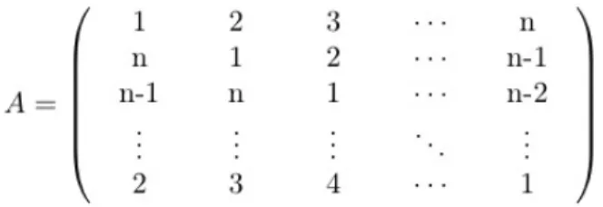
Figure 5. The matrix A that allows to reproduce heuristic IILSC from IISCS. The value of each cell A[i,j] is the length of the interval that begins with the gene at the position i in the genome and ends with the gene at the position j.
Gene expression data for E. coli are from the Gene Expression Omnibus [7]. The experiment used in this paper is GDS2580, but other data were used for replication (GDS2578, GDS2584, GDS2585, GDS2586, GDS2587, GDS2588, GDS2589, GDS2590, GDS2591).
D. Matching operons
To quantify the functional interest of our measure, we are interested by matching common intervals of genes with operons. We consider an operon as a transcription unit that contains at least two genes, and may include more than one promoter. We get those transcription units from Ecocyc [8] for E. coli.
A given interval of genes is a non operonic interval (NOI) when there exists no operon whose set of genes is a subset of the set of genes in the interval. On the contrary the interval is a partially operonic interval (POI) when there exists a collection of operons whose set of genes is a subset of the set of operonic genes in the interval, and the interval is a full operonic interval (FOI) when there exists a collection of operons whose set of genes is the set of operonic genes in the interval. Based of this measure, we will say that an interval of genes contains at least one operon when the interval is a POI or a FOI, and an interval contains no operon when the interval is a NOI.
May be common intervals have no more operonic meaning than any other set of intervals of genes. In order to compare the maximal common intervals, obtained via the IILCS algorithm, with any other, we generated 100 random sets of intervals. Let ICM be the set of maximal common
intervals nx be the number of maximal common intervals of
length x and X the set of lengths of the different maximal common intervals. The set ICR of random intervals is
obtained by taking randomly, in genome G1, nx intervals with
the length x, ∀ x ∈ X. Thus, ICR contains the same number of
intervals of the same length as ICM.
III. RESULTS/DISCUSSION
A. Operonic interest of the maximal common intervals
As an application, we applied the above protocol on
E. coli and V. cholerae genomes. The computation of all
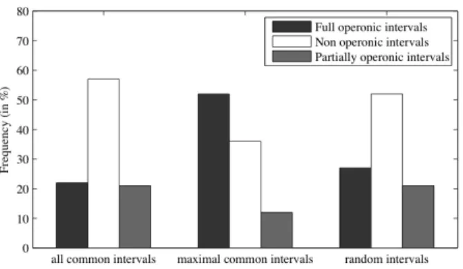
common intervals give us 11504 common intervals. As shown in Figure 6, only 43% of all common intervals contain at least one operon (FOI + POI). Similarly, the IILCS algorithm shows 325 maximal common intervals in which 74% contain at least one operon. When compared with the 100 intervals randomly produced (of similar size with those produced by IILCS), the results are similar (48%) than those obtained considering all common intervals, which confirms the interest of maximal common intervals from a functional point of view. As a natural consequence, maximal common intervals are then good candidates for applying a IILCS refinement as described above in the IISCS algorithm.
B. IISCS algorithm application results
The IISCS algorithm application gives a similar number of common intervals (318 and 317 when applied respectively with metabolic and co-expression information). Despite this
obvious similarity between the IILCS and IISCS results, the IISCS algorithm shows the great advantage to associate a score (either metabolic or co-expression like) to each common interval. It gives us the opportunity to select the most interesting intervals based on a given omics knowledge. After a parameter fitting process (data not shown), we consider a common interval as interesting when its score is above 0.6. In that case, 30 intervals reach the cut-off in a metabolic context, whereas 86 intervals are selected in a co-expression one.
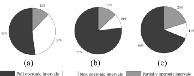
As previously done for the IILCS maximal common intervals, we establish the operonic interest of the selected intervals. Figure 7 illustrates the corresponding results. The functional refinement of the common intervals is obvious using the IISCS algorithm (i.e. from 74% (FOI + POI) to respectively 90% and 89% of intervals with an operonic meaning in a metabolic and co-expression context). In proportion, we obtain less NOI in both omics contexts. Furthermore, note that when one compares both contexts, only 13 intervals are selected in either metabolic and co-expressed-like.
C. Operon prediction vs. functional insights
IISCS results sound accurate from a functional viewpoint when compared to the bacterial operons. Therefore, passing from the functional meaning of intervals to the computational prediction of operons is very tempting. Operon prediction methods are evaluated in function of two measures [9]. The first, called sensitivity, relies on the rate of the number of accurately predicted within operon gene pairs on concrete within operon gene pairs. In other words, higher the sensitivity is, more the technique is efficient to recognize the gene composition of operons. The second, called
specificity, relies on the rate of the number of accurately
predicted transcription unit border gene pairs on concrete transcription unit border gene pairs. Higher the specificity is, more the method accurately delimits the operon borders. When applied on E. coli, the maximal common intervals show 45.47% sensitivity and 21.43% specificity. IISCS in a metabolic context emphasizes 30.26% sensitivity and
Figure 6. Proportion of common intervals that are (1) full operonic intervals, (2) non operonic intervals and (3) partially operonic intervals for all common intervals, maximal common intervals and random intervals.
12.48% specificity. IISCS in a co-expression context shows 18.75% sensitivity and 15.39% specificity.
Thus, the IISCS heuristic is obviously a bad computational operon predictor. However, few common intervals (30) correspond to 50 operons in metabolic context, which implies that common intervals contain a more complex organization than just a unique operon per interval. As an example, IISCS provides an interval composed by four operons (fepDGC, fepB, entS, entCEBA-ybdB). It is important to notice herein that all these four operons are co-regulated by common activators: Crp and Fur. fepDGC and
fepB products compose a unique ABC transporter, which
indicates the functional and essential relationship of these two operons, corroborating their common selection within an interval. Moreover, entS operon is divergent or antagonistic to fepDGC, which reinforces the intuition of common intervals composed by functional units instead of a unique operon. Note again, that such a complex structure may not be predicted using standard computational operon predictors.
IV. CONCLUSION
We proposed herein a technique that combines comparative genomics algorithms and omics data. As already pointed out in [2], such an integration significantly improves
the functional understanding of genomes comparison. As mentioned above, this integrated genomics approach is not appropriate to predict operons as other standard methods, but emphasizes functional units (themselves composed by operons more or less conserved among species) and their respective organizations in terms of gene rearrangements. Beyond the simple help to the genome annotation, this information is useful to discriminate functional units conserved from one species to another that might be further investigated using systems biology techniques and other modeling approaches.
REFERENCES
[1] S. Angibaud, D. Eveillard, G. Fertin, and I. Rusu, “Comparing bacterial genomes by searching their common intervals,” in Proc. 1st Bioinformatics and Computational Biology conference (BICoB 2009), ser. LNBI, vol. 5462. Springer, 2009, pp. 102–113.
[2] L.-Y. Chuang, J.-H. Tsai, and C.-H. Yang, “Binary particle swarm optimization for operon prediction,” Nucleic Acids Research, vol. 38, no. 12, p. e128, Jul 2010.
[3] M. Remm, C. Strom, and E. Sonnhammer, “Automatic clustering of orthologs and in-paralogs from pairwise species comparisons,” J. Molecular Biology, vol. 314, pp. 1041–1052, 2001.
[4] D. Sankoff, “Genome rearrangement with gene families.” Bioinformatics, vol. 15, no. 11, pp. 909–917, 1999.
[5] J. Tang and B. M. E. Moret, “Phylogenetic reconstruction from gene-rearrangement data with unequal gene content.” in Proc. Workshop on Software Architectures for Dependable Systems, ser. LNCS, vol. 2748. Springer, 2003, pp. 37–46.
[6] S. Angibaud, G. Fertin, I. Rusu, and S. Vialette, “A pseudo-boolean general framework for computing rearrangement distances between genomes with duplicates,” Journal of Computational Biology, vol. 14, no. 4, pp. 379–393, 2007.
[7] R. Edgar, M. Domrachev, and A. E. Lash, “Gene expression omnibus: NCBI gene expression and hybridization array data repository,” Nucleic Acids Research, vol. 30, no. 1, pp. 207–10, Jan 2002.
[8] P. D. Karp, M. Riley, M. Saier, I. T. Paulsen, J. Collado-Vides, S. M. Paley, A. Pellegrini-Toole, C. Bonavides, and S. Gama-Castro, “The ecocyc database,” Nucleic Acids Research, vol. 30, no. 1, pp. 56–58, 2002.
[9] H. Salgado, G. Moreno-Hagelsieb, T. F. Smith, and J. Collado-Vides, “Operons in escherichia coli: genomic analyses and predictions,” Proc Natl Acad Sci USA, vol. 97, no. 12, pp. 6652–7, Jun 2000.
(a) (b) (c)
Figure 7. Full operonic intervals, partially operonic intervals and non operonic intervals proportion for each common intervals experiment : common intervals obtained by (a) the IILCS method, (b) the IISCS method in metabolic context with a genomic density cutoff of 0.6 and (c) the IISCS method in the GDS2580 experiment context with a cutoff of 0.6 in interval expression score.