FACULTÉ DES SCIENCES Rabat
Faculté des Sciences, 4 Avenue Ibn Battouta B.P. 1014 RP, Rabat – Maroc Tel +212 (0) 37 77 18 34/35/38, Fax : +212 (0) 37 77 42 61, http://www.fsr.ac.ma
N° d’ordre : 2660
THESE DE DOCTORAT
Présentée parABDELJALIL LBADAOUI
Discipline : PHYSIQUE Spécialité : SISMOLOGIEBODY WAVES TOMOGRAPHY FROM OBS-RECORDED
EARTHQUAKES IN THE GULF OF CADIZ
Soutenue le 8 Juillet 2013
Devant le jury Président :
Mohammed Ouadi BENSALAH P.E.S Faculté des Sciences, Rabat
Examinateurs :
Abdallah EL HAMMOUMI P.E.S Faculté des Sciences, Rabat
Hamid BOUABID P.H Faculté des Sciences, Rabat
Aomar IBEN BRAHIM P.E.S CNRST Rabat
2
ACKNOWLEDGEMENTS
This work was carried out in the Mechanics Laboratory under the direction of Professor Abdallah EL HAMMOUMI of the Faculty of Sciences of Rabat and in the National Institute of Geophysics in the National Centre for Scientific and Technical Research of Rabat, under supervision of Professor Aomar IBEN BRAHIM.
First and foremost, I want to thank my advisor professor Abdallah EL HAMMOUMI of the faculty of sciences of Rabat, who guided me through all the difficulties in my research and provided me huge supports and several ideas about how to thinks and to solve scientific problems and how to be a real researcher.
My thank goes also to all members of the dissertation committee, professors Mohammed Ouadi BENSALAH and Hamid BOUABID of the faculty of sciences of Rabat.
Special thank for Professors Aomar IBEN BRAHIM and Azelarab EL MOURAOUAH, for their assistance and moral support, and encouragements for challenges. I learned from them a great knowledge and patience. Their passion and persistence in science imprint in my mind and will inspire me in the future.
3 TITLE
BODY WAVES TOMOGRAPHY FROM OBS-RECORDED EARTHQUAKES IN THE GULF OF CADIZ
ABSTRACT
The gulf of Cadiz is a region considered as a complex seismic area, where strong earthquakes occur and where the plate boundary between the African and Eurasian plates is not exactly known. we use high resolution seismic data recorded by a network of ocean bottom seismometers stations in the Gulf of Cadiz as well as eight Portugal land seismic stations. The OBS network was deployed within an experiment of the NEAREST project. Nearly 600 seismic events are extracted from the recorded data set and their analysis revealed that most of them occur at 20 to 80 km depths, with clusters of seismicity that occur mainly at the Gorringe Bank, within the SW segment of the Horseshoe fault and the Marques de Pombal Plateau and the S. Vicente Fault. A new NW-SE trend of seismicity has been revealed with depths that extend from 35 to 80 km. This seismicity trend is close and nearly parallel to the SWIM faults lineament. We present the first regional-scale high resolution P- and S-velocity distributions across the Gulf of Cadiz region. These velocity models are obtained using 3D seismic tomography to invert the OBS data-set. The results show that the patterns of anomalies in the Gulf of Cadiz are in general, oriented in NE-SW and NW-SE directions. They also show the presence of a low velocity zone (LVZ) to the SE of our study area. At shallow depth, this LVZ is interpreted as due to a large accumulation of sediments within the accretionary wedge, while at a greater crustal depth, it may reflect a continental crustal composition rather than an oceanic crust. Moreover, seismic velocity profiles show that under this region of the Gulf of Cadiz, the Moho averages a 30-km depth. The Gorringe Bank and the Marquise de Pombal plateau are found to be deeply rooted features and represent expressions of mantle uplifting.
KEYWORDS
4 TITRE
TOMOGRAPHIE DES ONDES DE VOLUME DEPUIS DES TREMBLEMENTS DE TERRE ENREGISTRES PAR DES OBS DANS LE GOLFE DE CADIX
RESUME
Le golfe de Cadix est une région considérée comme une zone sismique complexe. Dans ce travail, nous utilisons les données sismiques enregistrées par un réseau de stations OBS déployées dans cette région et par huit stations sismiques portugaises. 600 événements sont détectés et analysés. La sismicité est principalement remarquée au Banc de Gorringe au sud ouest de la faille Horseshoe, au niveau du plateau Marques de Pombal et de la faille Sao Vicente. Une orientation nord-ouest/sud-est de la sismicité a été révélée avec des profondeurs qui s'étendent de 35 à 80 km. Nous avons présenté des modèles tomographiques des ondes de volume. Ces modèles de vitesses sont obtenus en utilisant la tomographie sismique 3D par inversion de l'ensemble des données enregistrées. Les résultats montrent que les anomalies sont orientées dans des directions ouest/sud-est et nord-est/sud-ouest. Ils montrent également la présence d'une zone de faibles vitesses (LVZ) au sud-est de la région étudiée. Les profils des vitesses obtenus montrent un soulèvement du manteau au niveau de la faille Sâo Vicente coïncidant avec le plateau Marques de Pombal. Ils montrent de plus que le Moho sous le golfe de Cadix est plutôt profond, avec une profondeur moyenne d'environ 30 km en aval de la surface de l’océan. En outre, une zone nord-ouest/sud-est de grandes vitesses est localisée au sud-ouest de notre zone d'étude.
MOTS CLEFS
5 RESUME DETAILLE
Depuis une dizaine d'années, de nombreuses études ont été menées en tomographie sismique pour établir une image de l'intérieur de la Terre et de comprendre la structure géologique de certaines régions parmi les plus complexes du monde. Cependant, aucune étude d'imagerie tomographique à base des ondes de volume avec des données OBS n’a été réalisée dans le golfe de Cadix. Le principal objectif du travail présenté dans cette thèse est de mener une étude détaillée permettant de déterminer un modèle de tomographie sismique locale dans le golfe de Cadix. La zone étudiée est caractérisée par un aspect géologique très complexe, résultant de la convergence des plaques africaine et eurasienne, où de violents séismes se produisent et où la limite entre les plaques africaine et eurasienne n'est pas toujours exactement connue. Ce travail a été réalisé en utilisant des données sismiques de très haute résolution obtenues par un réseau sous-marin de stations OBS déployées dans le golfe de Cadix ainsi que par huit stations sismiques terrestres situées au Portugal. Le réseau OBS a été déployé dans le cadre du projet NEAREST.
Les images tomographiques des perturbations de vitesse en trois dimensions ont été réalisées par inversion des temps d’arrivée des ondes sismiques de volume élaborées à partir de sismogrammes, par détermination des différentes phases. Le système d'analyse sismologique SEISAN a été utilisé pour localiser plus de 600 événements survenus pendant cette période. Parmi lesquels le ML = 4.8 du 1er Janvier 2008 ,événement sismique qui présente la plus grande magnitude enregistrée par le réseau OBS et les stations sismiques Portugaises considérée durant cette période d'observation .Grace au réseau OBS, nous avons détecté un nombre important d'événements locaux qui n'ont pas pu être identifiés précédemment avec les réseaux sismiques Marocain, Espagnol et Portugais. Le grand nombre de tremblements de terre enregistrés au cours de cette période d'une année montre que le golfe de Cadix est une zone très active, en raison de la convergence entre les plaques et parce qu’il est réparti sur une vaste zone de déformation.
Dans notre cas, la sismicité se situe au nord de la zone des failles SWIM ; elle est concentrée au niveau de trois principaux blocs : au sud du banc de Gorringe, la partie sud de
6
la plaine abyssale de Horseshoe, et au nord,nord-ouest de la faille de Horseshoe, le long du plateau Marques de Pombal et la faille Sâo Vicente. Quelques tremblements de terre se sont produits dans la zone du prisme d'accrétion, et une sismicité dispersée est observée au sud du bassin d'Algarve et du banc de Portimâo. La distribution en profondeur des hypocentres varie entre les catégories peu profonds et profondeur intermédiaire ; la majorité des événements enregistrés ont entre 20 et 80 km de profondeur.
Nos résultats montrent une orientation NW-SE de la sismicité qui traverse la faille du Horseshoe. Cette sismicité observée au sud de notre zone d'étude, parallèlement à la SFZ peut donc être corrélée à l’ensemble des failles SWIM. La première section verticale montre trois principaux blocs de tremblements de terre : le long du banc de Gorringe, la faille de Sao Vicente et le sud du banc de Potimâo, tandis que le second profil montre que la sismicité se concentre dans deux principaux domaines : au niveau banc de Gorringe et de la faille du Horseshoe. La faille inverse du Horseshoe présente une pente d’environ 50 km de longueur. L'inversion des temps d’arrivée est un processus itératif qui requiert un modèle de référence. Dans ce travail, nous l’avons initialisé à l’aide du modèle proposé par l’équipe de recherche du projet NEAREST , 2008. Ce modèle a été, par la suite, amélioré (Matias, et al., 2009). Tous les événements enregistrés sont, ensuite, localisés par ce modèle de vitesse initiale avec une amélioration en utilisant l’algorithme VELEST (Kissling, et al., 1994). Ce dernier est constitué d'une croûte comportant trois couches avec une interface à environ 6 km de profondeur, et la discontinuité du Moho à environ 26 km de profondeur.
L’algorithme tomographique LOTOS-10 conçu pour l'inversion simultanée des ondes P et S, a été utilisé dans ce travail. Nous avons défini les paramètres de l’amortissement et de l’effet du bruit de fond en effectuant une série de tests synthétiques. De plus, un réglage sélectif des données a été effectué, dans certaines régions. Ce test montre une excellente zone de couverture entre 15 et 45 km de profondeur. Le paramétrage du domaine a été réalisé avec la construction du maillage par le réglage de la distance entre les nœuds à 5 km. Cet algorithme utilise la méthode dite de pseudo-bending pour le traçage des rais. Elle permet l’estimation de la trajectoire la plus courte des rais : le rai initial est perturbé alors que les points source et récepteur sont maintenus fixes (Nolet,. 2008). Le code LOTOS
7
utilise cette approche pour le traçage des rais avec une légère modification (Koulakov, 2009). Les rais construits de cette manière ont tendance à voyager à travers les anomalies de grandes vitesses et éviter les modèles à faibles vitesses. Avant l’inversion, nous avons effectué plusieurs séries de tests synthétiques afin d'obtenir un paramétrage optimal et d'évaluer la fiabilité des modèles tomographiques. Le test synthétique est une technique qui permet d'examiner la résolution des données utilisées, le test montre que les anomalies périodiques sont reconstruites dans la plupart des régions de la zone d'étude, et la résolution est beaucoup plus élevée dans la zone délimitée par le banc de Gorringe à l'ouest du Cap Sao Vicente au nord, du banc de Portimao à l'Est et la ligne dorsale du Coral dans le sud. En plus du test du damier, nous avons effectué le test odd/even pour donner plus de crédibilité aux résultats tomographiques. Cet essai montre une bonne corrélation des résultats dans la plupart des zones du golfe de Cadix. Les structures tridimensionnelles y révèlent une limite marquante entre les différentes anomalies de haute et basse distribution de vitesse, soit dans une direction NE-SO ou dans des directions NW-SE. Nous remarquons, en outre que les tomogrammes des ondes P et S montrent une distribution de vitesses plus ou moins semblables.
Délimitée en latitudes par 35,1 ° N et 37 ° N et en longitudes par 8 ° W et 10 ° W, une grande anomalie négative dans la direction SE est mise en évidence. Elle peut être expliquée par la présence d'une zone à forte concentration de sédiments. A de grandes profondeurs, cette anomalie pourrait être interprétée comme une zone de forte réflexion. Cette partie du golfe de Cadix est plutôt faite de la croûte continentale et donc, sa partie nord délimite plus ou moins la limite entre les croûtes océanique et continentale. Nos résultats montrent une ceinture NW-SE des anomalies de grande vitesse s'étendant à partir du banc de Gorringe jusqu’au prisme d'accrétion traversant la plaine abyssale de Horseshoe. Cette ceinture suit environ le SWIM (SFZ), présentant un ensemble de failles de décrochement comme il a été prouvé précédemment. On constate en plus une zone de transition qui présente une séparation claire de deux structures. Cela peut être interprété comme le résultat d'une déformation de compression oblique de l’Ibérie par rapport à la plaque Nubie. Notre modèle montre aussi une large anomalie positive, s'étendant sur 50 km à l'ouest de la profondeur du Cap Sao Vicente. Cette anomalie est assez claire, la distribution des anomalies de vitesse des
8
ondes S y est presque similaire à celle des ondes P. Elle peut être associée à un soulèvement du manteau profond. Des profils tomographiques verticaux ont été réalisés dans lesquels nous présentons les vitesses réelles au lieu des leurs perturbations. Ces profils montrent un soulèvement du manteau au niveau de la faille Sâo Vicente coïncidant avec le plateau Marquis de Pombal. Ils montrent de plus que le Moho sous le golfe de Cadix est plutôt profond, avec une profondeur moyenne d'environ 26 km en aval de la surface de l’océan. Au NW de la zone d'étude, une anomalie distincte de grande vitesse s'étend à partir de 10 km à 35 km de profondeur et coïncide à peu près avec le soulèvement du banc de Gorringe. En dessous de ces profondeurs, cette anomalie à grande vitesse continue à apparaitre mais semble plutôt atténuée, ce qui confirme les résultats d’une récente étude (Jiménez, Munt et al 2010), En outre, la coupe verticale de tomographie montre clairement que le banc de Gorringe est une anomalie qui implique un soulèvement du manteau et que cette caractéristique topographique émerge d’une profondeur considérable à partir du manteau. L’orientation W-E du banc de Portimao où une anomalie de grande vitesse est observée, est expliquée à la fois, par la convergence oblique des plaques et par l’existence d'une activité sismique récente. La partie de la plaine abyssale Horseshoe que nous étudions est proche de la frontière entre l’Eurasie et la plaque africaine. Cette région est fortement influencée par un mouvement de compression. Les images tomographiques de la partie nord de la plaine abyssale Horseshoe montrent une anomalie de faible vitesse séparant deux blocs d’anomalie positive le long de l’alignement SWIM où l'activité sismique est faible. Cette anomalie peut, sans aucun doute, être interprétée comme la zone de contact entre la faille Horseshoe et les failles de l’alignement SWIM. Certains auteurs soutiennent l'existence d'une zone de subduction active sous le golfe de Cadix, les données GPS n'ont, par contre, montré aucun mouvement différentiel à travers le détroit de Gibraltar (Stich et al, 2006; Serpelloni et al, 2007). En fait, pour des profondeurs inférieures 50 kilomètres, nos profils de vitesse ne montrent aucune indication de la zone de subduction au SE de la zone d'étude.
9 TABLE OF CONTENT Acknowledgements ... 3 abstract ... 4 Resumé ... 5 Résumé détaillé ... 6 Liste of figures ... 13 List of tables ... 18 General introduction ... 19
PART1 LITERATUREREVIEW 1. Introduction ... 22 2. THEORY OF ELASTICITY ... 23 2.1 Displacement vector ... 24 2.2 Strain tensor ... 25 2.3 Stress tensor ... 26 2.4 Equation of motion ... 28
2.5 Stress strain relation ... 29
2.5.1 Fluid material (zero viscosity) ... 29
2.5.2 Elastic material ... 29 2.6 Wave equations ... 30 2.7 Body waves ... 31 2.7.1 Longitudinal waves ... 31 2.7.2 Transverse Waves ... 32 2.8 Surface waves ... 33 2.8.1 Rayleigh Waves ... 35 2.8.2 Love waves ... 41
2.8.3 Love waves in a layer on a half space ... 41
2.7.4 Boundary conditions... 43 3. EARTH STRUCTURE... 45 3.1 The crust ... 47 3.2 The mantle ... 48 3.3 The core ... 49 3.4 Tectonic plates... 50
3.5 Convection and the earth’s mantle ... 53
3.5.1 Where tectonic plates meet ... 54
4. EARTHQUAKES ... 56
4.1 Where do earthquakes happen ? ... 59
4.2 Seismographs ... 61
4.3 Seismograms ... 62
4.4 Phase nomenclature ... 64
10
4.5.1 Teleseismic earthquakes ... 66
4.5.2 Regional earthquakes ... 67
4.5.3 Local earthquakes ... 68
5. WHAT IS SEISMIC TOMOGRAPHY? ... 69
5.1 The main steps to image earth interior ... 72
5.2 Imaging the earth with seismic data ... 74
5.2.1 Travel time tomography ... 74
5.2.2 Example of travel time tomography ... 80
6. INVERSE PROBLEM ... 82
6.1 Travel time inverse ... 83
6.2 Why inverse problems are hard? ... 87
6.3 Earthquakes location ... 87
6.2.1 Example location of earthquake in homogenous medium ... 92
7. CONCLUSION... 95
PART 2 BODY WAVES TOMOGRAPHY IN THE GULF OF CADIZ 1. INTRODUCTION ... 97
2. MOTIVATION AND RESEARCH OBJECTIVES... 99
3. THE GULF OF CADIZ STUDY AREA ... 100
4. RAY TRACING AND TRAVEL-TIMES INVERSION ... 105
4.1 The Eikonal equation ... 106
4.1.1 Eikonal equation for fluid mediums ... 106
4.1.2 Eikonal Equations in Isotropic Elastic Mediums ... 108
4.2 Ray geometry ... 111
4.2.1 Ray solution in layered mediums ... 112
4.2.2 Inversion of travel time ... 118
4.2.3 Shortest travel-time path ... 121
4.3 Bending method ... 123
4.3.1 Pseudo bending method ... 125
5. SEISMICITY OF THE GULF OF CADIZ ... 129
5.1 Nearest Project ... 129
5.2 Data format ... 134
5.3 Seisan analysis software ... 134
5.4 Seismicity ... 136
5.5 Inversion method and procedure ... 140
6.5.1 Using the LOTOS code ... 145
5.5.2 One dimensional velocity optimization and preliminary source location algorithm ... 146
5.6 Starting velocity model ... 148
6. SYNTHETIC TESTS ... 152
7. RESULTS AND DISCUSSION ... 158
7.1 Swim lineaments (SFZ) ... 165
7.2 Sâo Vicente Canyon ... 167
11
7.4 Portimao-Bank ... 175
7.5 Horseshoe Abyssal Plain ... 176
8. conclusion ... 178
9. References ... 180
APPENDIX 1. Least squares method ... 188
2. Snell’s law ... 192
3. Pane wave ... 194
4. Conversion of format seisan to lotos ... 196
12 LISTE OF FIGURES
Figure 1.1 Displacement of two neighboring point P and Q Figure 1.2 Stress tensor
Figure 1.3 Displacement shape produced by compressional waves propagation. Figure 1.4 Displacement shape produced by shear waves propagation.
Figure 1.5 Three component seismogram showing the surface waves phases, of earthquake , Rayleigh wave are observed in vertical and radial component, whereas Love waves are shown in transverse component. Figure 1.6 The particle motion for surface waves (Rayleigh waves), (P. Shearer, 2009). Figure 1.7 The shape of displacement variation with depth shows that displacement is
exponentially decreasing with depth.
Figure 1.8 The particle motion for surface waves (Love waves), (P. Shearer, 2009). Figure 1.9 Love waves in a half space.
Figure 1.10 A cross section through earth, showing the thicknesses of each layer, dividing the earth in three main layers ( the crust, the mantle and the core). Figure 1.11 A cross section through earth , showing detailed earth structure, (1)
Continental crust, (2) Oceanic Crust , (3) Subduction Zone, (4) Upper Mantle, (5) Volcanic Eruption, (6) Lower Mantle ,(7) Panache Material Warmer ,(8)Outer Core, (9) Inner Core, (10) Cells Mantle Convection, (11) Lithosphere, (12) Asthenosphere, (13) Discontinuity Gutenberg, (14) Discontinuity Mohorovicic.
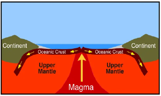
Figure 1.12 Map show the crustal plates boundary (Stein and Wysession, 2003). Figure 1.13 Picture shows the process of the Sea floor spreading.
Figure 1.14 Convection in the mantle drives plate tectonics .(www.geo .m tu. edu/~hamorgan/ bigideas welc-o me.html).
Figure 1.15 Stress builds until it exceeds rock strength.
Figure 1.16 Agadir earthquake February 29, 1960, killed some 12,000 people and injured 12,000 others. Destruction of the old part of the city was complete, and some 70% of the new structures in the city were destroyed (http://mimoun1.forumavie.com).
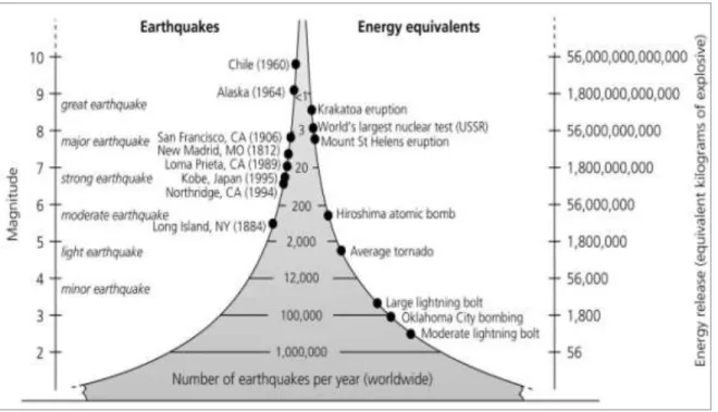
Figure 1.17 Comparison of frequency, magnitude, and energy release of earthquakes. (Stein and Wysession., 2003).
Figure 1.18 30 years seismicity map of earthquakes magnitude greater than four, shows that most events occur along the boundaries between tectonic plates, (Stein and Wysession, 2003).
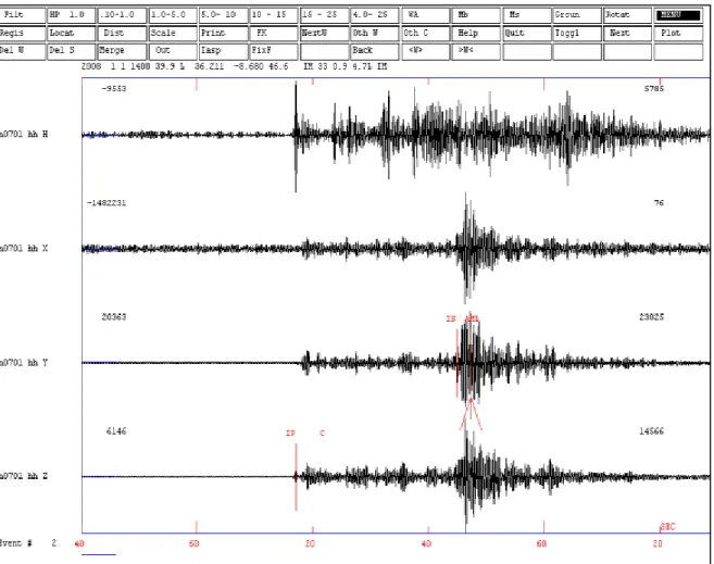
Figure 1.19 First teleseismic record of earthquake of April 17 1889 in Japan , enregistred by the Geodetic institute Potsdam (http://www.gfz-potsdam.de/portal/gfz). Figure 1.20 Three component seismogram showing the body and the surface waves
phases of the earthquake occurred in Gulf of cadiz in August 1 , OBS 1. Figure 1.21 Seismograms showing the differences in amplitudes and frequencies
between an earthquake occurred in India in April 4, 1995 of magnitude 4.8 (bleu signal) and an nuclear test occurred again in Indian in may 11, 1998 ,magnitude 5.1 ( red signal), data are recorded at Nilore, Pakistan (Stein and Wysession, 2003).
13
Figure 1.22 The 1994 Northridge earthquake recorded at station OBN in Russia. Some of the visible phases are labeled (Shearer, 2010).
Figure 1.23 Examples of seismic rays and their nomenclature. The most commonly identified phases used in earthquake location are the first arriving phases: P and PKIKP (Stein and Wysession, 2003).
Figure 1.24 Teleseismic earthquake of may 2008 (China), M= 8.0, recorded by OBS 12 (all components). The seismic phases continued for more than 6000 Seconds. Long period surface waves (Rayleigh & Love) are also recorded. Figure 1.25 Part of seismogram showing a regional earthquake of june 8/ 2008 (Greece)
recorded by OBS 12 (all components), M= 6.5.
Figure 1.26 Part of seismogram showing a local earthquake (all OBS’s vertical components) of November 1st, 2008 (Greece), M=4.8 (SW Iberia).
Figure 1.27 Global Seismographic Network (IRIS).
Figure 1.28 Travel time picks for various body waves phases and travel time curves, the data are 57655 travel times from 104 sources (earthquakes and explosions). ( Kennett and Engdahl, 1991).
Figure 1.29 An example ray path in a 3-D block velocity perturbation for Tomography problems.
Figure 1.30 Travel time plot of the P seismic waves of the events occurred in morocco between 1993 to 2003 recorded by Moroccan seismic station networks. Figure 1.31 An example ray path and cell numbering scheme for a simple 2-D
tomography problem.
Figure 1.32 An example ray path and in 2-D dimension showing the blocs where the basis function is none zero.
Figure 1.33 2-D block geometry velocity perturbation for an idealized tomography problem, the model consists on identical blocks , traversed by 13 ray paths.
Figure 1.34 Chart showing the differences between the inverse and forward problem. Figure 1.35 Geometry for an earthquake location in earth with variance change in
velocity with depth.
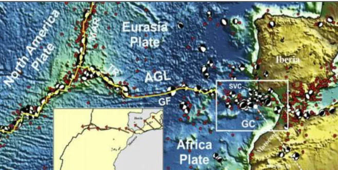
Figure 2.1 Plate tectonic interactions between the southern Eurasia and the North Africa plates with the main elements of plate boundaries superimposed: AGL: Azores–Gibraltar Line; GC: Gulf of Cadiz; GF: Gloria Fault; MAR: Mid-Atlantic Ridge; TR: Terceira Ridge. Solid yellow line: plate boundaries (Zitellini et al 2009).
Figure 2.2 Gulf of Cadiz region offshore SW Iberia, showing the bathymetry map and existing faults, SWIM is South West Iberian Margin faults lineament (Duarte, et al 2009).
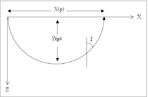
Figure 2.3 Geometry of the ray segment along a path from a surface source to a surface receiver
Figure 2.4 Incidence angle of a ray Figure 2.5 Incidence angle of a ray
Figure 2.6 Polar coordinate system for a ray in equatorial plan Figure 2.7 Ray path in spherical earth model.
14
Figure 2.9 An example of a shortest path followed by a seismic ray traveling from a source S to receiver R.
Figure 2.10 Piece of the path shown in Figure (2.17).
Figure 2.11 Process of bending algorithm used to determinate the shortest path. Hatched light grey patterns represent negative anomalies of -30%; dark grey patterns are positive anomalies of +30%. (Koulakov, 2009).
Figure 2.12 Tangential, normal and anti-normal unit vectors along the ray path (Kazuki et al,. 1997)
Figure 2.13 Three point perturbation scheme used in pseudo bending method, Um & Thurber (1987).
Figure 2.14 Seismicity of the Gulf of Cadiz as recorded between august 2007 and July 2008 as shown by the red dots;, GB : Gorringe Bank , CP: Coral Pach, , SVC: Sâo vicente Canyon, RV : Rharb Valley , PB: Portimâo Bank, AB: Algarve Bassin, AJB: Alentijo Bassin , Ocean Bottom Seismometers (OBS) blue triangles and Portugal Land stations green triangles.
Figure 2.15 Ocean Bottom Seismometer’s on board, (Zitellini N., Carrara G. & NEAREST Team. - ISMAR Bologna Technical Report, June 2009).
Figure 2.16 Location of the broad band stations used in this study, ocean Bottom Seismometers (OBS) blue triangles and Portugal Land stations green triangles.
Figure 2.17 Seismicity of the Gulf of Cadiz as recorded between august 2007 and July 2008 as shown by the black circles; AB: Algarve Bassin, AJB: Alentijo Bassin the inclined blue line represents the SWIM faults zone (SFZ), and red lines are the possible faults.CP: Coral Pach, GB : Gorringe Bank , GF : Gorringe fault , HsF : horseshoe fault ,MPF : Marques de Pombal fault , PB: Portimâo Bank, PSF: Pereira de Sousa fault, RV : Rharb Valley , SVC: Sâo vicente Canyon, SVF: Sâo vicente fault,
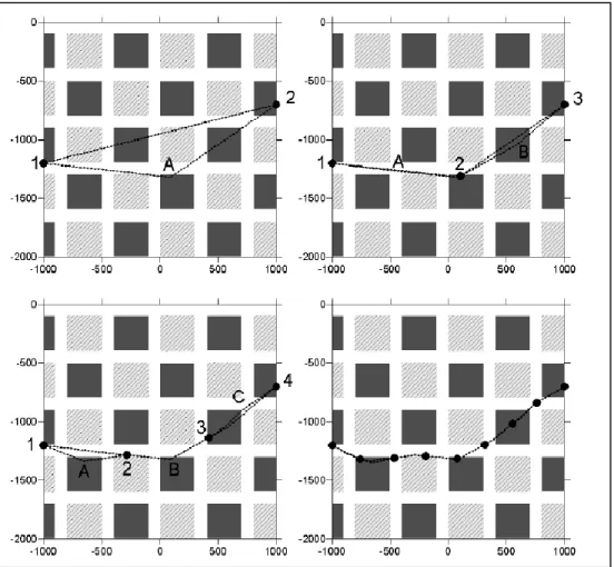
Figure 2.18 Seismic profiles shown in the map Figure (2.9), showing events that occurred within 40 km distance from the profile. This profile indicates a more continuous pattern of seismicity. HsF: Horseshoe fault, GB: Gorring Bank.
Figure 2.19 Seismic profiles shown in the map Figure (2.26), showing events that occurred within 40 km distance from the profile, this shows three separate clusters of seismicity. AW: Accretionary wedge, GB: Gorring Bank , SVF: Sao Vicente fault.
Figure 2.20 Seismic profiles shown in the map Figure (2.26), showing events that occurred within 40 km distance from the profile, this shows three separate clusters of seismicity. AW: Accretionary wedge, GB: Gorring Bank , HsF: horsechoe Fault.
Figure 2.21 Chart showing the General structure of the LOTOS code working process. Figure 2.22 Ray paths in the map view at depth of 20, 40, 60 and 80 Km showing the
coverage paths, purple point are the stations.
Figure 2.23 Ray paths in the map view in a vertical cross section shown by grey dots. Blue triangles are the stations.
15
cruise survey.
Figure 2.25.a Velocity model obtained by the VELEST algorithm , the black line plot represent the model given by OBS location , the red line represent the model given using both OBS’s and Portugal land station and the blue model is given using only the Portugal land stations.
Figure 2.25.b Different starting P-velocity models used for optimization of the initial velocity model; model 1 is the velocity model proposed in the
NEAREST-2008 cruise report, model 3 is the model derived using VELEST, while models 2,4,5,6 and 7 are initial-velocity models with slight modifications of the previous ones.
Figure 2.26 Checkerboard test performed for P and S waves in horizontals sections. Figure 2.27 Synthetic test performed for P and S waves in horizontals sections at 35 Km
depth.
Figure 2.28 Checkerboard test performed for P waves in vertical sections, AA’ and BB’ shown in Figure below.
Figure 2.29 Checkerboard test performed for S waves in vertical sections, AA’ and BB’ shown in Figure below.
Figure 2.30 Anomalies of P velocities distribution, test with inversion of two independent data subsets (with odd/even numbers of events).
Figure 2.31 Anomalies of P velocities distribution, test with inversion of two independent data subsets (with odd/even numbers of events).
Figure 2.32 P-velocity distribution at 10 km. Solid lines show the existing faults and dotted lines show possible strike-slip faults, and black dots show the epicenters location given by tomography program and inclined gray line represent the SWIM fault zone (SFZ).
Figure 2.33 P-velocity distribution at 15 km. Solid lines show the existing faults and dotted lines show possible strike-slip faults, and black dots show the epicenters location given by tomography program and inclined gray line represent the SWIM fault zone (SFZ).
Figure 2.34 P-velocity distribution at 25 km. Solid lines show the existing faults and dotted lines show possible strike-slip faults, and black dots show the epicenters location given by tomography program and inclined gray line represent the SWIM fault zone (SFZ).
Figure 2.35 P-velocity distribution at 35 km. Solid lines show the existing faults and dotted lines show possible strike-slip faults, and black dots show the epicenters location given by tomography program and inclined gray line represent the SWIM fault zone (SFZ).
Figure 2.36 P-velocity distribution at 50 km. Solid lines show the existing faults and dotted lines show possible strike-slip faults, and black dots show the epicenters location given by tomography program and inclined gray line represent the SWIM fault zone (SFZ).
Figure 2.37 S-velocity distribution anomalies at 10 km. Solid lines show the existing faults and dotted lines show possible strike-slip faults, and black dots show the Epicenters location given by tomography program and inclined gray line represent the SWIM fault zone (SFZ)
16
faults and dotted lines show possible strike-slip faults, and black dots show the Epicenters location given by tomography program and inclined gray line represent the SWIM fault zone (SFZ).
Figure 2.39 S-velocity distribution anomalies at 25 km. Solid lines show the existing faults and dotted lines show possible strike-slip faults, and black dots show the Epicenters location given by tomography program and inclined gray line represent the SWIM fault zone (SFZ)
Figure 2.40 S-velocity distribution anomalies at 35 km. Solid lines show the existing faults and dotted lines show possible strike-slip faults, and black dots show the Epicenters location given by tomography program and inclined gray line represent the SWIM fault zone (SFZ)
Figure 2.41 S-velocity distribution anomalies at 50 km. Solid lines show the existing faults and dotted lines show possible strike-slip faults, and black dots show the Epicenters location given by tomography program and inclined gray line represent the SWIM fault zone (SFZ)
Figure 2.42 Horizontal sections of P-velocity anomalies at 15,25,35,50 km depth. (perspective view)
Figure 2.43 Horizontal sections of P-velocity anomalies at 15,25,35,50 km depth. (perspective view)
Figure 2.44 NW-SE belt of high velocity anomaly (SWIM lineament)
Figure 2.45 Horizontal P-velocity distribution at 25, 35 and 50 km, showing high velocity anomaly southwest Portuguese Margin.
Figure 2.46 Positions of the vertical cross-sections velocity profiles 1 and 2
Figure 2.47 P velocity distribution in vertical cross-sections 1, the position of vertical section is shown in the Figure (2.39)., GB: Gorringe Bank. HsF: Horseshoe Fault
Figure 2.48 P velocity distribution in vertical cross-sections 2, the position of vertical section is shown in the Figure (2.39), SVF : Sao Vicente Fault, AW : Accretionary wedge.
Figure 2.49 Horizontal P-velocity distribution at 25, 35 and 50 km, showing the attenuation of anomaly A between the Gorringe bank and horsechoe abyssal plain.
Figure 2.50 Density and temperature depth profiles at four positions identified in Fig (2.26): Tagus Abyssal Plain (profile a), Gorringe Bank (profile b), and Horseshoe Abyssal Plain (profiles c and d), (Jiménez, Munt et al 2010). Figure 2.51 Figure (3.5) Anomalies of P velocities distribution, test with inversion of
two independent data subsets (with odd/even numbers of events).
Figure 2.52 Figure (3.4) Checkerboard test performed for S waves in vertical sections, AA’ and BB’ shown in Figure below.
Figure 2.53 Model results showing the lithosphere structure. The map above show the position of the profile. White dots are earthquake hypocenters, (Jiménez, Munt et al 2010).
Figure 2.54 P- velocity distribution in vertical cross-sections 1, shows the layers going to 50 km depth , precising the direction in which the African oceanic lithosphere thrust Eurasian plate.
17
Figure 2.55 Horizontal P-velocity distribution at 25, 35 and 50 km, showing high velocity anomaly in the Porimaô Bank.
Figure 2.56 Horizontal P-velocity distribution at 25, 35 and 50 km, showing low velocity anomaly in the N-W of the horseshoe Abyssal Plain.
Figure 3.1 a projection in subspace, p is the projection in column space, d is the data vector and e is the error vector. b) Illustrate the projection of the data vector in terms of components, showing the error quantities and is an outlier.
Figure 3.2 A plane wave incident on a horizontal surface, is the incidence angle, denote the length of the ray.
Figure 3.3 A plane wave crossing a horizontal interface between two homogeneous half-spaces.
Figure 3.4 Propagation of plane wave. Figure 3.5 Chart of processing method
Figure 3.6 Resolution Kernel (Badal et al 2003).
LISTE OF TABLE
Table 1.1 Earthquakes with 70 000 or more deaths (http://earthquake .usgs.gov). Table 1.
Table 1.1 2 P and S velocities in the reference 1-d model after optimization by the Lotos software.
18 GENERAL INTRODUCTION
Nowadays, the plate tectonics theory provides several models trying to explain the major geological features of the present structure of our planet. This theory proposes that the current deformation of the lithosphere is related to several internal processes inside the earth. For few a decades, many research studies have been conducted in seismic tomography to image the interior of the Earth and to understand the most complex geological structure of the globe. Recently, the development and improvement of equipments in several domains, as well as advances in computer studies (processing power, memory capacity), in electronic (more sensitive sensors) have contributed significantly to obtain more explicit models of the earth. However, it is known that the resolution of tomographic models is limited by a number of factors, including the distribution of seismogenic zones and seismological networks scattered around the world. The seismotectonic context does not always allow the investigation of some complex areas by non-destructive methods. Before that, it was too difficult to investigate the oceans underground, since the sensors are often located only on the continental zones; the non-uniform distribution location of these sensors makes the ray tracing to be a difficult task. The direct result of these limitations is that the regions of low coverage have often lower resolution models. Seismic tomography is a still widely used method of exploring the earth interior, although the gravimetric measurements and morphological studies of bathymetry (Zitellini et al, 2009), (Gutscher et al, 2002), (Gracia et al, 2010) begin to show their importance, and the international community is naturally oriented towards tomographic techniques for determining the basement velocity structure. These techniques have been field proven in the continental, and marine seismic application did not require major changes.
The main objective of the work presented in this thesis is to undertake a detailed study that will help produce a local seismic tomography model of the south West region of the Gulf of Cadiz, which is an area characterized by a complex geology, resulting from the convergence of the African and Eurasian plates.
19
The local seismic tomography studies of this offshore zone requires in general that the stations must be in the same study area, thus, achieving a tomographic studies based on the data collected by land stations can never reveal the detailed structure of the region. In August 2007, a European research consortium team decided to make detailed studies of the western zone of the Gulf of Cadiz, in the project nearest (integrated observations from near shore sources of tsunamis: towards an early warning system) which is an eu-funded project (goce, contract n. 037110) mainly addressed to the identification and characterisation of large potential tsunami sources located near shore in the Gulf of Cadiz, and to realize a quantitative understanding of lithosphere processes.
Since, it was necessary to carry out seismic measurements at sea; the broad band seismic stations have been installed in the Atlantic Ocean, since, a glimmer of hope will begin to emerge, then we were assured that we will use a worthwhile quality feedstock, the National Center for Scientific and Technical Research (CNRST) in Rabat, participated to this project by accomplishing a tomographic study of the region by exploiting the data collected in the ocean. A tremendous amount of work was made, and incredible patience is needed to extract all the seismic events that occurred in this period, thorough job was carried out when analyzing earthquakes, knowing that good location leads to successful tomographic models. Often seismic tomography need a large database to get an excellent coverage, however, having a huge amount of data can be misleading sometimes about the reality reality of the earth interior. We have exploited more than 600 events in this study, which is an enormous database for an excellent coverage. After that, our database is prepared for inversion process, containing all the epicenters and arrival times of all recorded earthquakes; we examined several inversion methods, to choose the adapted method for our data inversion and to avoid accumulation of errors by applying appropriate algorithms, the most recent methods and systems have been used, for example we have chosen ray tracing algorithms that use methods of integration instead of differentiation. We showed results from 10 km depth, as we will see after, from this depth rays coverage begin to be excellent, it means that there are still 5.2 km of the crust needs to be investigated, because of deepest station is in about 4.8 km deep, we plan to study this layer
20
applying a surface wave tomography rather than body waves, by determination of velocity models for shallow structure, using the Rayleigh waveforms which depend strongly on the shallow velocity structure of the medium, which is used to obtain the group-velocity dispersion curve (Dziewonski et al., 1969), and applying the digital filtering with a combination of Multiple Filter Technique (Dziewonski et al 1969), (Badal et al, 1992), (Chourak et al, 2003).
21
Literature review
Part
1
CHAPTER OUTLINE 1. Introduction 2. Theory of elasticity 3. Earth structure 4. Earthquakes
5. What is seismic tomography? 6. Inverse problem
22
1. Introduction
Seismology is the multi-variant discipline that can never be understood without dealing with the theory of elasticity. During the Master studies we have carried out several notions to deeply understand this theory, which allows me to penetrate in theoretical concepts of seismology. The theory of elasticity solved several seismological problems even if approximations are sometime needed for simplifying. Accordingly, basic concepts and principles, dealing with stresses and strains were used to establish relationships applicable to different types of mediums; however, they do not allow the resolution of complex problems. That is why scientists introduce other concepts to define cases of the ideal material, so even if the continuum mechanics are not able to examine the true nature of matter, it’s still establishing different laws of behavior of real materials. We know that the surface of the earth, where we are living is constantly shaken, because of the movement of the plates, sometimes is violently shaken during earthquakes, causes then a human disaster. We describe in this thesis the main processes of the dynamics of the planet consists of various internal layers that are in constant motion, and the causes of these disasters. Great progress for the development of seismic instrumentation in recent years has greatly helped geophysicists to perform great tomographic models. But it’s not always easy to estimate the parameters of inverse problems, seismic tomography models are mainly resolved by inverting the travel time of the different phases, and they need often a great effort in the estimation of parameters, and powerful algorithms for matrix inversion, because often the amount of data exceeds the number of model parameters, we are dealing here with an inverse problem which consists of determining the internal state of unknown system, based on a given quantities of observations, knowing the structure of the system. Inverse problems are present in almost sciences and engineering, and they are applied when you search for information on a system without being able to measure directly. In this part we will explain how we can solve an inverse problem using a mathematical approach.
23
2. Theory of elasticity
The theory of seismic waves is based on the theory of elasticity. This theory is closely related to the development of the seismology. Regarded on Hook’s discovery, Navier was the first how present the equations for equilibrium and motion of elastic solid, and investigate the general equations of the theory of elasticity. Development of theory of elasticity was largely due to the work of Cauchy and Poisson when they worked on the propagation of light, in 1831 Poisson found that, at large distance from source of disturbance (not the case at the present with sophisticated instruments) the motion transmitted by the fast wave was longitudinal, followed by a transverse wave that is the slowest one. After that Stokes demonstrate in 1845 that the displacement of matter was irrotational dilatation, and the slower wave was a wave of equivoluminal distortion with elements rotations, he made the observation that resistance to compression and resistance to shearing are the two fundamental kinds of elastic resistance by introducing the modulus of compressibility and rigidity.
Forty two years later, Lord Rayleigh discovered that a specific wave can be formed near the free surface of homogeneous body propagating along the surface with a different velocity, and decay with a depth, he found that this wave is elliptically polarized in the plane determined by the normal to the surface and by the direction of propagation. Since, it is the discovery of Rayleigh waves; 24 years later Love called them “Rayleigh waves” after he discovered them theoretically. This entire exploit, has been discovered by several mathematicians and scientists long before any seismic records were obtained, in this thesis we will develop the theory for more understanding the process of wave propagation, and the elastic constitutive equations and equations of motion in Cartesian coordinates. All these results can be found in several textbooks, (Love 1944), (Fung 1965), (Takeuchi and Saito, 1972), (Aki and Richard, 1980), (Thorne lay terry c. Wallace, 1995), (Seth Stein and Michael Wysession, 2003), (P. Shearer, 2009) and (Novotny, 1999).
24 2.1 Displacement vector
Consider a particle at point P (original state) , which is moved to point P’ (deformed state, the position of the vector y depends on the one of x, therefore
(1,1)
Under the condition of continuity, we notice the existence of the inverse function
According to Lagrange description of motion, the displacement is given by –
In a neighborhood of the P point, let's consider another point Q, displaced to the point Q’ in the deformed state Figure (1.1)
Figure 1.1 Displacement of two neighboring point P and
25
Using the Taylor expansion we obtain
, (1.4)
Where and using the Einstein’s summation convention
So, we can get
2.2 Strain tensor
From the displacement field we can derive the strain field; we take the straightforward approach, assuming that if only the small strains are considered (Ewing et al 1957). The distance between P and Q is and the square of this distance can be expressed as
From the quadrangle (PP’QQ’) and Equation (1.6)
26
Can be expressed in term of components
Consequently
We consider: and the quantity S
with and we introduce , the strain tensor can be expressed as
Strain is the formal description of the change in shape of a material, if we neglect the non-linear terms we get the Cauchy’s infinitesimal strain tensor
2.3 Stress tensor
The stress vector is defined by
27
Figure 1.2 Stress tensor.
Where is the effect of all surface forces exerted across the element of surface . Let
be the stress vector acting on this element, this vector can be
expressed on tensor notation as where , are the components of
the stress tensor. Applying the condition of equilibrium yield
Using the Cauchy’s formula
Applying the Gauss theorem
And putting , where A is a continuous vector with continuous derivatives and v is
the unit outward normal, may be expressed as a volume integral
28
If the integral assumed to be equal to zero, this yield
Eq. is known as the equation of the equilibrium.
2.4 Equation of motion
The equation of motion can be obtained by adding the inertial force , we define
is the density, v the velocity and t is the time, the total derivative with respect to time is equal to the corresponding partial derivative
where u is the displacement. The equation of motion of a continuum mechanics can be expressed in this form
Taking in account the approximation assuming that the products of the derivatives are small we get
29 2.5 Stress strain relation
2.5.1 Fluid material (zero viscosity)
The stress tensor is defined in a fluid material of zero viscosity as
2.5.2 Elastic material
The stress tensor is defined in elastic material of zero viscosity as
is the material constant.
In an isotropic Earth the elasticity tensor involves only two constants, the bulk modulus and the shear modulus (Nolet 2008).
where so,
where is the volume dilatation, is the shear modulus and has no immediate physical interpretation. Such laws can be very complicated, but are greatly simplified when we ignore the hysteresis caused by anelastic effects and when we confine ourselves to very small displacements. In that case the medium deforms approximately linearly with the applied stress. We replace (1.22) into the Equation of motion (1.18)
For a homogeneous isotropic medium, the elastic coefficients are constant, than (1.23) can be written as
30 It is known that So (1.23) become
Representing the equation of motion in terms of components of displacement vector
Finally, if we replace we deduce the equation of motion well-known in seismology, from which we shall derive the wave equations
2.6 Wave equations
From the previous equation , than we neglect the body forces F, this equation can take the form
Applying the divergence operator yield
and , equation (1.29), become
31
Where is the velocity of compressional waves, and if we applying the curl operator to the equation (1.28), we get the vector wave equation
Where is the velocity of shear waves.
The purpose of the following is to give a precise explanation of the theory of propagation of elastic waves, it also defines essential mathematical formulas for understanding the physics of waves propagations, and we will deal with the different types of waves that propagate in different elastic media.
2.7 Body waves
It follows from the theory of elasticity that there are two principal types of elastic body waves, Includes the P and S waves, and the wavefront makes a spherical shape when the body waves propagate in elastic medium.
2.7.1 Longitudinal waves
Also called compressional or irrotational waves; in seismology we call them the primary waves or just P waves, because they are the fastest waves, so they are the first appearing on seismograms, longitudinal waves undergo an volume change, as the waves propagates, the displacements in the direction of waves propagation cause material to be alternately compressed and expanded. The irrotational waves are thus generated by a scalar potential. The solutions for P and S waves like those given in equation and give the locations of wave-fronts, when P-wave emerges from deep in the Earth to the surface, a fraction of it is transmitted into atmosphere as sound waves. Such sounds, if frequency is greater than 15 cycles per second, are audible to animals or human beings. These are known
32
as earthquake sound (J.R. Kayal, 2008), for it cannot describe all wave phenomena. These approximations are collectively known as geometric ray theory and are the standard basis for seismic body-wave interpretation.
Figure 1.3 Displacement shape produced by compressional waves propagation.
2.7.2 Transverse Waves
also called shear, rotational or secondary waves (S waves), when these waves pass through elastic medium they involve shearing and rotation of material without any volume changes, the displacement associated with propagating shear wave is perpendicular to the direction of wave propagation.
33
The velocities of longitudinal waves and the transverse waves in homogeneous and isotropic medium, satisfy the Hook’s law, are given by the formulas
,
where is the shear modulus, is the Lamé coefficient, and is the density. Poisson relation assumes the fact where the coefficients are equals, this relation is often used in seismology to describe many elastic materials, involve that
Both longitudinal and transverse waves can propagate in solid media, but only primary waves can propagate in fluid medium when . Elastic body waves are reflected and transmitted at the discontinuities of elastic parameters; in fact we observe increases the number of waves on seismograms.
2.8 Surface waves
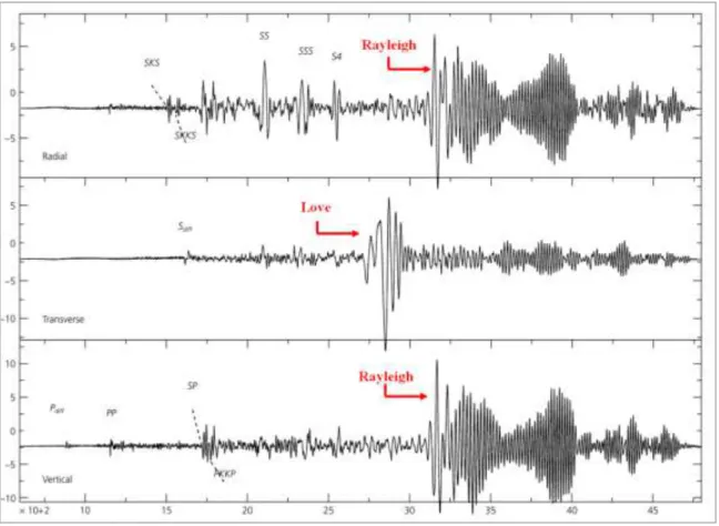
We have seen that the body waves can propagate in a homogeneous, isotropic and unbounded medium. If the medium is bounded, another kind of waves can be guided along the surface of the medium. The Surface waves are the waves that propagate along a boundary and whose amplitudes go to zero as the distance from the boundary goes to infinity. There are two basic types of surface waves, Love and Rayleigh waves, named after the scientists who studied them first. Love’s work was directed to the explanation of waves observed in horizontal seismographs, while Rayleigh predicted the existence of the waves with his name. The main difference between the two types of waves is that the motion is of SH type for Love waves, and of P–SV types for Rayleigh waves. Love and Rayleigh waves show a large surface wave train arriving on a seismometer’s Figure (1.5); transverse component shows the arrival of Love waves, followed by Rayleigh waves on a vertical and radial component, which are distinguished from each other by the types of particle motion in their wave fronts. In the description of body waves, the motion of particles in the wavefront was resolved into three orthogonal components – a longitudinal vibration parallel to the ray
34
path (the P-wave motion), a transverse vibration in the vertical plane containing the ray path (the vertical shear or SV-wave) and a horizontal transverse vibration (the horizontal shear or SH-wave). These components of motion, restricted to surface layers, also determine the particle motion Figure (1.6) and Figure (1.8) and character of these two types of surface waves.
Figure 1.5 Three component seismogram showing the surface waves phases, of
earthquake , Rayleigh wave are observed in vertical and radial component, whereas Love waves are shown in transverse component.
After a large earthquake, contrary to the body waves whose energy spreads three dimensionally, the surface waves can circle the globe many times, and their energy spreads tow dimensionally and it’s concentrated near the earth surface.
35 2.8.1 Rayleigh Waves
In 1885 Lord Rayleigh described the propagation of a surface wave along the free surface of a semi-infinite elastic half-space. The particles in the wavefront of the Rayleigh wave are polarized to vibrate in the vertical plane Figure (1.6). The resulting particle motion can be regarded as a combination of the P- and SV-vibrations
Figure 1.6 The particle motion for surface waves (Rayleigh waves),
(Adapted from , Shearer, 2009).
It is well known that a general transient wave can be expressed as a superposition of harmonic waves by means of the Fourier integral (Novotny, 1999). And by the superposition of harmonic waves of different amplitude and frequencies, we can construct rather complicated wave shapes as well as seismic surface waves. If we consider a wave field in term of potential component, from the equation of motion for a homogeneous isotropic
36
medium equation , the displacement field can be decomposed into scalar potential and vector potential .
And express components of displacement vector in terms of potentials
In the case of the wave field independent of the y-coordinate
On the other hand we can obtain from 1 and 1 22 the components of the stresses acting in the perpendicular plan of z axis are
And from the components of displacement vector we see that the perpendicular plan of propagating plan contains and , whereas is in thus, the wave field can be decomposed into two parts, and express the vector potential as
37
where represent the displacement in plan and
represent the displacement in plan.
Consider the potential for longitudinal waves, , and the potential for transverse waves, , in the form of plane harmonic waves, moving with constant velocity and without change of shape, propagating in the -direction. The displacement vector can then be decomposed as
Where and , for part of wave the components
and equals zero, hence the displacement is
where and can be defined as
where is a given angular frequency, and are unknown functions, describing the depth-dependent amplitudes, we now replace in the wave equations and we get
These two equations represent the equations of harmonic oscillator, which can be easily resolved, the solutions take the form
,
38
Can be decomposed into, and
Where is the wave number.
Or in the this form
In witch and describes the decomposition of surface wave into two body waves, (Novotny, 1999), ( C. A. Coulson, 1977), replacing into
and
we can now express the stress components by inserting the displacement components into stress formula , the stress components can then be written as follow
We have calculated the stress component to use them, for those further boundary conditions, the stress components equals zero in the free surface of
39
The amplitudes diminish with the depth increase for
If the apparent velocity (see plane waves in the Appendix) the
, are real, thus and goes to infinity, which no agree
with the second boundary condition, we have to consider the case to avoid this problem and take the imaginary part of and .
The amplitudes now take the form
Or in this simple form
for that and increase to infinity for infinite depth, this terms doesn’t represent any physical meaning, so we keep
The terms for
putting Become now
These equations show that the waves are exponentially decreasing with depth increase. Figure (1.47) represents the vertical and horizontal displacements calculated for a given value of poison coefficient, these displacements are normalized with respect to the vertical displacement of the particle motion in the surface.
40
Figure 1.7 The shape of displacement
variation with depth shows that displacement is exponentially decreasing with depth.
Now shall we determine the quantities and, from the displacement expression given by the equations , displacement vector can take the form
And the stress component become
Inserting expressions of and into , when the boundary conditions are satisfied for stresses , we finally arrive at system of linear equations with unknowns and ,
41
The solution of this system of linear equation yield the Rayleigh velocity For typical values of Poisson solid, for more details see (Novotny, 1999) and (Stein and Wysession, 2003).
2.8.2 Love waves
The boundary conditions which govern the components of stress at the free surface of a semi-infinite elastic half space prohibit the propagation of SH-waves along the surface. However, A.E.H. Love showed in 1911 that if a horizontal layer lies between the free surface and the semi-infinite half-space.
Figure 1.8 The particle motion for surface waves (
Love waves), (P. Shearer, 2009).
2.8.3 Love waves in a layer on a half space
Love wave are a surface waves result from interaction of SH waves, this type of waves require an increasing velocity with depth, if not the case Love waves cannot exist.
42
Figure 1.9 Love waves in a half space.
The displacement of the particle motion associated with propagation of Love waves can be expressed as where
43
Where , and is the wave number.
2.7.4 Boundary conditions
We consider the following boundary conditions, the stress components equals zero in the free surface of
in , all stresses and displacements are continuous;
when the displacement go to zero , if the apparent velocity
is real, thus go to infinity, which no agree with the boundary condition, we have to consider the case to avoid this problem and take the imaginary part and .
44
The first boundary condition is satisfied when
So,
The second and third boundary conditions yield again a system of linear equations with unknowns and .
where
45
3. Earth structure
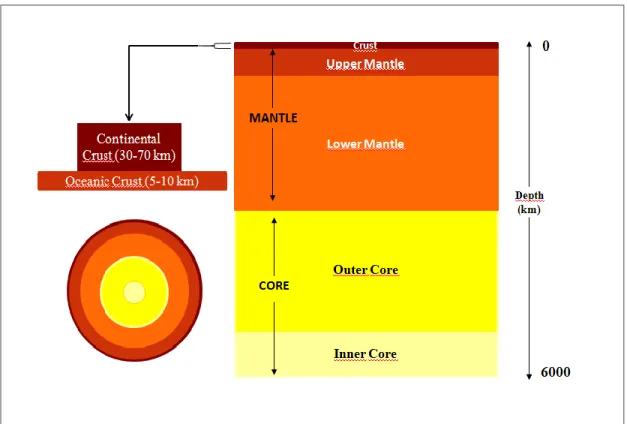
The earth is composed of several layers. The inner core in the extreme center is a solid iron and nickel ball located about 6370 km from the surface of the earth. And outer core in form of the ring, formed of a fluid mixture of molten iron and nickel. The core is surrounded by the asthenospher composed of a portion of the mantle and the crust (oceanic or continental) Figure (1.10). It is well known that the Earth has a molten core, what is now general knowledge was slow to develop. In order to explain the existence of volcanoes, some nineteenth century scientists postulated that the Earth must consist of a rigid outer crust around a molten interior. It was also known in the last century that the mean density of the Earth is about 5.5 times that of water (Lowrie, 2007). From this it was inferred that density increased towards the Earth’s center under the effect of gravitational pressure.
Figure 1.10 A cross section through earth, showing the thicknesses of each layer, dividing the
46
The key to modern understanding of the interior of the Earth is density, pressure and elasticity was provided by the invention and improvements of sensitive seismographs. The progressive refinement of this instrument and its systematic employment world-wide led to the rapid development of the modern science of seismology. Important results were obtained early in the twentieth century. The Earth’s fluid core was first detected seismologically in 1906 by R. D. Oldham. Resent geophysical studies have revealed that the Earth has several distinct layers. Each of these layers has its own properties Figure (1.11).
Figure 1.11 A cross section through earth , showing detailed earth structure, (1)
Continental crust, (2) Oceanic Crust , (3) Subduction Zone, ,(4) Upper Mantle, (5) Volcanic Eruption. , (6) Lower Mantle ,(7) Panache Material Warmer ,(8) Outer Core, (9) Inner Core, (10) Cells Mantle Convection, (11) Lithosphere , (12) Asthenosphere, (13) Discontinuity Gutenberg , (14) Discontinuity Mohorovicic. (Wikipedia).
47 3.1 The crust
Earth outermost layer, the crust preserves a memory of the Earth’s evolution that extends back more than 3.4 Gy, while today it is well established that silicic material extracted from the mantle forms an outer crust and it’s well documented now a compromise aspects of the physical state of the planet and its evolution and the Earth's crust when many seismological studies performed early from the beginning of the last century brought important elements of the overall appearance and global view of the structure of the crust. Recently, using high frequency resolutions of deep seismic reflection profiling (Meissner,1973. Oliver et al, 1976, Clemperer 1989) and wide-angle reflection profiling investigations (Healy et al., 1982, W.D. Mooney, 1985) understanding the crustal structure began to change radically when all studies showed that the crust is highly heterogeneous in composition and physical properties, furthermore, the large number of collected data and the increasing improvements of seismic station network in the last 40 years played a key role in determining the first model of the crust, an important works mentioning soil crusts have made, and regional crustal thickness models were created by several scientists (Mohorovicic, 1910), (Conrad 1925), (Byerly 1926), (Byerly and Dyk, 1932), (Gutenberg 1932), (DeGolyer, 1935), (Heiland, 1935), (Press, 1964), (Crampin, 1964), (Kovach and Anderson, 1964), (Christensen, 1965), (Dix, 1965), (Audry and Rossetti, 1962), (Aubert and Maignien, 1948), (Leprun, 1978), (Pindell 1985)… Seismology began to have several successful discovery, for example when has succeed to discern the petrological boundary between ultramafic and silicic rocks, where the wave velocity increases by about 6.5 km/s (in the lower crust) to more than 7.7 km/s (upper mantle), (James and Steinhart, 1966). The crust varies in thickness. It is thin (about 7 km) under oceans, thicker (about 40 km) under continents, and thickest (as much as 70 km) under high mountains. The continental crust is made up mostly of low-density granitic rocks and that no granite exists on the floor of the deep ocean, the crust there consists entirely of basalt and gabbro overlay by sediments (Grotzinger et al., 2007). As a result of plate tectonics Figure (1.12), the oceanic crust and continental crust differ systematically in their main physical properties, including density, thickness, age and composition. Continental crust has an average thickness of , the density of , and an average age of , whereas the oceanic crust has an average