Decision map for spatial decision making in urban planning

DECISION MAP FOR SPATIAL DECISION MAKING IN URBAN PLANNING

Salem CHAKHAR PhD

LAMSADE

Université Paris Dauphine

Place du Maréchal de Lattre de Tassigny, 75775 Paris Cexex 16 France Tel: +33 1 44 05 49 18 Fax: +33 1 44 05 40 91 E-mail: chakhar@lamsade.dauphine.fr Vincent MOUSSEAU Professor LAMSADE

Université Paris Dauphine

Place du Maréchal de Lattre de Tassigny, 75775 Paris Cexex 16 France Tel: +33 1 44 05 41 84 Fax: +33 1 44 05 40 91 E-mail: mousseau@lamsade.dauphine.fr Clara PUSCEDDU PhD

University of Architecture of Alghero Alghero (SS) Sardinia - Italy E-mail: clara.pusceddu@uniss.it

and LAMSADE

Université Paris Dauphine

Place du Maréchal de Lattre de Tassigny, 75775 Paris Cexex 16 France Tel: +33 1 44 05 44 01 Fax: +33 1 44 05 40 91 E-mail: pusceddu@lamsade.dauphine.fr Bernard ROY Professor LAMSADE

Université Paris Dauphine

Place du Maréchal de Lattre de Tassigny, 75775 Paris Cexex 16

France

Tel: +33 1 44 05 42 88 Fax: +33 1 44 05 40 91 E-mail: roy@lamsade.dauphine.fr

Abstract: This paper introduces the concept of decision map and illustrates the way this concept can be used for spatial decision making in urban planning. The decision map is defined as an advanced version of conventional geographic maps which is enriched with preferential information

and especially destined to “visual” spatial decision making. The concept of decision map as defined here is a generic tool that may be used for several purposes. This paper focuses on the general aspects of the decision map. It also briefly shows how the concept of decision map can be extended to support collaborative and communicative spatial decision making.

Keywords: Decision map, ELECTRE TRI, GIS, Collaborative spatial decision making

1 INTRODUCTION

Spatial decision problems in urban planning are generally of multicriteria nature, where several, often conflicting, evaluation criteria should be taken into account for evaluating different development policies. The conflicting aspects that characterize both the objectives and preferences of all the participants in the decision process, and the evaluation criteria that should be considered reduce substantially the chance to reach a solution supported by all the participants in the decision process.

Therefore, scientific research on spatial decision making in urban planning is now increasingly required (i) to take into consideration the multicriteria nature of spatial problems that decision makers have to tackle; (ii) to make possible interaction of point of views from various actors with various actors and stakeholders involved in the spatial decision process in a collaborative way (Healey, 1997); (iii) to provide an adequate environment for supporting integration of expert and experiential knowledge from local communities in a communicative way (Innes, 1995; Healey, 1992); and (iv) to focus attention on the decision context escaping from generality and universality.

Different large scale models, mostly originated in the fields of operational research and economics (e.g. linear programming, optimisation techniques, cost-benefit analysis) have been proposed to deal with spatial decision problems in urban planning (see Batty (1994) for a review), and especially in transportation problems. Most of these models have at least one of the following limitations (see also Lee, 1973): they (i) do not permit to represent complexity of spatial problems to decision makers; (ii) neglect social, qualitative and interactive dimensions, of importance in the spatial decision making process; (iii) do not take into account the spatial dynamics; and (iv) do not support in their operational dimension communicative and collaborative decision making.

Starting from this, the objective of this paper is thus to introduce a new concept called decision map and illustrate the way this concept can be used for spatial decision making in urban planning. The decision map is defined as an advanced version of conventional geographic maps which is enriched with preferential information and especially destined to “visual” spatial decision making. It looks like a set of homogenous spatial units; each one is characterized with a global, often ordinal, evaluation that represents an aggregation of several partial evaluation relative to different criteria. When it is effectively integrated into a geographical information system (GIS), the

decision map permits to avoid, fully or partially, several ones of the limitations of large scales models enumerated above.

The concept of decision map as defined here is a generic tool that may be applied in different domains (e.g. generation of potential alternatives, communication and participation). This paper focuses on the general aspects of the decision map and briefly shows how the decision map can be extended to support collaborative and communicative spatial decision making.

The rest of the paper is structured as follows. Section 2 introduces the concept of decision map and presents a procedure for its generation. Section 3 provides an illustrative example for the construction of a decision map. Section 4 compares our decision map concept to classical cartographic modelling. Section 5 extends the decision map to the context of collaborative and communicative spatial decision making. Section 6 concludes the paper. 2 CONCEPT OF DECISION MAP

2.1 Definition

The concept of decision map is an advanced version of conventional geographic maps which is enriched with preferential information and especially destined to “visual” decision making. More formally:

Definition. A decision map M is defined as {(u, f(u)):u∈U}, where U is a set

of homogenous spatial units (or zones) and f is a function defined as follows: f: U → E

u → f(u)= Φ[g1(u),…gm(u)]

where E is an ordinal scale, Φ is a multicriteria aggregation model and gi(u) is the performance of spatial unit u according to criterion gi.

Accordingly, a decision map summarizes the preferential information of the decision maker(s) relatively to a set of conflicting evaluation criteria into an ordinal information. In practice, criteria may represent physical data (e.g. slope) or not (e.g. aptitude for urbanization, vulnerability to pollution). Each criterion is represented as a thematic map composed of a set of homogenous spatial units. To each spatial unit, we associate one (ordinal or cardinal) evaluation relatively to a scale E. The construction of a decision map requires the aggregation of the different criteria maps into one final map that looks like a set of homogenous spatial units; each one is characterized with a global, often ordinal but it can be cardinal, evaluation that represents an aggregation of several partial evaluation relative to different criteria.

The construction of a decision map requires the subdivision of each criterion map into homogenous units. Description of territory in a set of spatial units is not new in land management (Joerin and Musy, 2000). In classical cartographic modelling, these units are often defined through census tracts or administrative and political boundaries. In this paper as in Joerin (1998) (see also Joerin and Musy (2000), and Joerin et al. (2001)), the initial subdivision of territory into homogenous units (Joerin uses the term zone instead of unit but the two terms are used indifferently in this paper) should respect the spatial

natural (forest, body of water) and human (highways, parks, buildings) boundaries. But the choice of homogenous units boundaries should be based on the nature of the spatial decision problem under consideration and should take into account different functional, non physical, spatial relationships that reflect the interdependence among the different spatial units. Thus, as extension of opportunities with representation with decision map, we shall envisage to consider as homogeneous unit, the territorial component in which economic, social, fiscal, historical and environmental aspects are strongly interconnected to each others.

2.2 Decision Map Generation Procedure

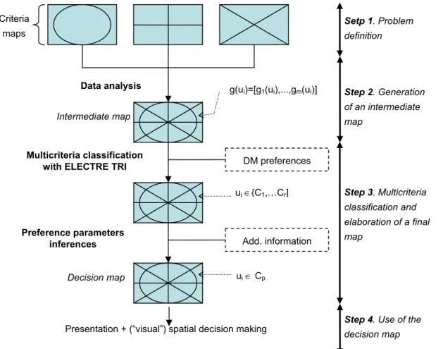
The procedure of decision map generation is illustrated in Figure 1. It is details in the following paragraphs.

2.2.1 Step 1: Problem Definition

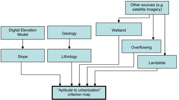
The first step for the construction of the decision map consists in the generation of criteria maps. Each criterion map represents a specific theme. As underlined above, criteria may represent natural phenomena or not. In the first case, the criterion map may be extracted from the data stored in the GIS through a series of simple transformations (e.g. reclassification, interpolation). For instance, a criterion map representing the slope may be obtained from the Digital Elevation Model. The definition of criterion maps of non real phenomena calls for more complex models and requires often the intervention of the analyst/expert to model the considered phenomena. Modelling may simply take the form of some additional information to incorporate into an existing data layer, or, often, to the creation of a new data layer. In this last case, the definition of the criterion map requires an overlay of several data layers. For instance, a criterion map of "Aptitude to urbanization" is obtained through the overlay of several data layers representing the following information: slope, lithology, wetland, overflowing and landslide.

A criterion map could incorporate also experiential knowledge of local communities. It is an important element in structuring and representing the decision context that decision maker has to tackle. Aspirations, beliefs, preference and value systems of local communities can support decision makers in the decision process, preventing potential conflicts.

Once the criterion map is generated, it is composed of a set of homogenous spatial units each one is characterized with one evaluation according to an ordinal or cardinal scale E. In practice, criteria are often of different types and may be evaluated according to different scales. Without loss of generality, in this paper we suppose that the criteria are evaluated on the same scale.

2.2.2 Step 2: Generation of an Intermediate Map

The next step consists in generating an intermediate map through the intersection of the criteria maps. The generated intermediate map is composed of a new set of spatial units which result from the intersection of the boundaries of the spatial units of the different criteria maps. Each spatial unit is characterized with a vector of m evaluations relative to the m criteria.

Formally, to each spatial unit u, we associate the vector [g1(u), g2(u),…,gm(u)]. To be able to perform the overlay operation, different criteria maps must represent the same territory and must be defined according to the same spatial scale and the same coordinate system.

2.2.3 Step 3: Multicriteria Classification and Elaboration of a Final Map To generate a final decision map, we should first use an aggregation mechanism to aggregate the vector associated with each spatial unit u in the intermediate map into one global evaluation. Mathematically, we write: g(u)= Φ [gj(u)] j∈F. F is the criteria family and Φ is the aggregation mechanism defined as follows:

Φ: Em _{→ E} [g1(u),g2(u),…,gm(u)] → Φ(u)

The aggregation mechanism Φ is a multicriteria sorting model permitting to assign each unit to one or several predefined categories on the scale E. In this paper, the multicriteria sorting model is ELECTRE TRI (see Yu, 1992). Ideally is to obtain a final map in which each spatial unit is assigned to exactly one class. Nevertheless, in practice this is difficult to obtain without additional information. Additional information are provided by the decision maker(s)/analyst(s) and may take the form of some assignment examples as in Mousseau and Slowinski (1998), a restriction of affectation of one or several units to some specific categories and/or an interdiction of other units to be assigned to some other categories.

The additional information will be the input of an inference model permitting to retrieve the preferential parameters of the sorting model (here ELECTRE TRI). This permits to reduce the cognitive effort of the decision maker. In this paper, we have adapted the inference model developed by Mousseau and Slowinski (1998) (also see Mousseau (2005)). Their approach starts with some simple assignment examples provided by the decision maker and then an optimisation algorithm is applied for inferring the required parameters from these assignment examples. This approach permits to construct the preference model that better resituate the aspirations of the decision-maker and reduce sensibly his/her cognitive effort. Finally, it is important to note that the additional information should not modify the consistency of the preference parameters. Often, several iterations are required to obtain pertinent additional information.

2.2.4 Step 4: Use of the Decision Map

Decision map as defined here is a generic tool that may be applied in different domains. It is devoted especially to clarify and support “visual” spatial decision making. It can be extended to support collaborative and communicative spatial decision making in urban planning as we will see in section 5.

Decision map may also be used to the generation of potential alternatives. In fact, in (multicriteria) spatial decision making, we generally represent potential alternatives through one of three atomic spatial entities, namely point, line or

polygon (Chakhar and Mousseau, 2003). Therefore, in a facility location problem, potential alternatives take the form of points representing different potential sites; in a linear infrastructure planning problem (e.g. highway construction), potential alternatives take the form of lines representing different possible routes; and in the problem of identification and planning of a new industrial zone, potential actions are assimilated to a set of polygons representing different candidate zones.

Using a decision map, point-based alternatives take simply the form of individual spatial units. These spatial units may be too large for locating a single point but this will reduce substantially the search space when a second phase is envisaged. In the same way, line and area-based alternatives are obtained as a set of linearly adjacent spatial units and a set of contiguous spatial units, respectively.

Criteria maps

Setp 1. Problem

definition

Data analysis _g(u

i)=[g1(ui),...,gm(ui)] _{Step 2. Generation} of an intermediate map

Intermediate map

Multicriteria classification _{DM preferences}

with ELECTRE TRI

Step 3. Multicriteria classification and elaboration of a final map ui∈{C1,…Cr] Preference parameters

inferences Add. information

ui ∈ Cp Decision map

Step 4. Use of the

decision map

Presentation + (“visual”) spatial decision making

Figure 1 Decision map generation procedure

3 ILLUSTRATIVE EXAMPLE

The following example permits a better appreciation of the way the decision map is generated. It is inspired from a real-world application provided in Braux (1996) which is relative to the valorisation of the Haute-Savoie region in the South-East of France. Only the three first steps are illustrated here. Note that for clarity, all the maps are represented through a regular girded form.

3.1 Step 1: Problem Definition

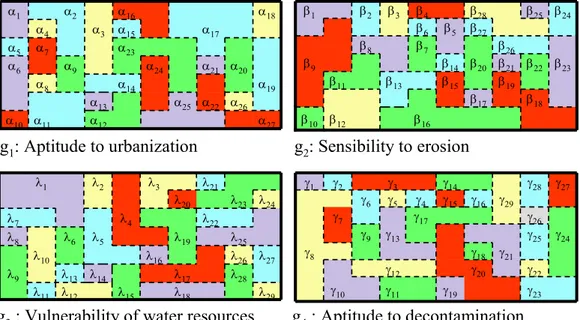
Four themes in relation with water resources and environment are to be evaluated (see Table 1). Both "Aptitude to urbanization" and "Aptitude to decontamination" criteria are to be maximized. The two other ones (i.e. "Sensibility to erosion" and "Vulnerability of water resources") are to be minimized. We suppose that all criteria have the same weight of 0.25 (but in practice they may have different weights.)

Table 1: List of criteria for the illustrative example

Criterion Description Max/Min Weight

g1 Aptitude to urbanization Max 0.25

g2 Sensibility to erosion Min 0.25

g3 Vulnerability of water resources Min 0.25

g4 Aptitude to decontamination Max 0.25

The process of generation of the "Aptitude to urbanization" criterion map is illustrated by the flowchart of Figure 2. Similar flowcharts are used to generate the other criteria maps. The criteria maps obtained are illustrated in Figure 3. We remark that these maps are not generated through a GIS. However, the generation of such maps are relatively simple operation in most of available GIS technology. Note also that the same five-level ordinal scale is used for the different criteria.

Other sources (e.g. satellite imagery)

Digital Elevation Wetland

Geology Model Overflowing Slope Lithology Landslide “Aptitude to urbanization” criterion map

λ₂₉ λ₁₈ λ₁₅ λ₁₂ λ₁₁ λ₂₈ λ₁₇ λ₁₄ λ₁₃ λ₉ λ₂₇ λ₂₆ λ₁₆ λ₁₀ λ₂₅ λ₁₉ λ₅ λ₆ λ₈ λ₂₂ λ₄ λ₇ λ₂₄ λ₂₃ λ₂₀ λ₂₁ λ₃ λ₂ λ₁ λ₂₉ λ₁₈ λ₁₅ λ₁₂ λ₁₁ λ₂₈ λ₁₇ λ₁₄ λ₁₃ λ₉ λ₂₇ λ₂₆ λ₁₆ λ₁₀ λ₂₅ λ₁₉ λ₅ λ₆ λ₈ λ₂₂ λ₄ λ₇ λ₂₄ λ₂₃ λ₂₀ λ₂₁ λ₃ λ₂ λ₁ β₁₆ β₁₂ β₁₀ β₁₈ β₁₇ β₁₉ β₁₅ β₁₃ β₁₁ β₂₃ β₂₂ β₂₁ β₂₀ β₁₄ β₉ β₂₆ β₇ β₈ β₂₇ β₅ β₆ β₂₄ β₂₅ β₂₈ β₄ β₃ β₂ β₁ β₁₆ β₁₂ β₁₀ β₁₈ β₁₇ β₁₉ β₁₅ β₁₃ β₁₁ β₂₃ β₂₂ β₂₁ β₂₀ β₁₄ β₉ β₂₆ β₇ β₈ β₂₇ β₅ β₆ β₂₄ β₂₅ β₂₈ β₄ β₃ β₂ β₁ γ₂₃ γ₁₉ γ₁₁ γ₁₀ γ₂₂ γ₂₀ γ₁₂ γ₂₁ γ₁₈ γ₈ γ₂₄ γ₂₅ γ₁₃ γ₉ γ₂₆ γ₁₇ γ₇ γ₂₉ γ₁₆ γ₁₅ γ₄ γ₅ γ₆ γ₂₇ γ₂₈ γ₁₄ γ₃ γ₂ γ₁ γ₂₃ γ₁₉ γ₁₁ γ₁₀ γ₂₂ γ₂₀ γ₁₂ γ₂₁ γ₁₈ γ₈ γ₂₄ γ₂₅ γ₁₃ γ₉ γ₂₆ γ₁₇ γ₇ γ₂₉ γ₁₆ γ₁₅ γ₄ γ₅ γ₆ γ₂₇ γ₂₈ γ₁₄ γ₃ γ₂ γ₁ α₂₇ α₁₂ α₁₁ α₁₀ α₂₆ α₂₂ α₂₅ α₁₃ α₁₉ α₁₄ α₈ α₂₀ α₂₁ α₂₄ α₉ α₆ α₂₃ α₇ α₅ α₁₇ α₁₅ α₃ α₄ α₁₈ α₁₆ α₂ α₁ α₂₇ α₁₂ α₁₁ α₁₀ α₂₆ α₂₂ α₂₅ α₁₃ α₁₉ α₁₄ α₈ α₂₀ α₂₁ α₂₄ α₉ α₆ α₂₃ α₇ α₅ α₁₇ α₁₅ α₃ α₄ α₁₈ α₁₆ α₂ α₁

g₁: Aptitude to urbanization g₂: Sensibility to erosion

g₃: Vulnerability of water resources g₄: Aptitude to decontamination

Scale for g1and g4

Scale for g2and g3

1 Very bad 2 Bad

3 Average 4 Good

5 Very good 4 Good 3 Average 2 Bad 1 Very bad

5 Very good

5 Very good 4 Good

3 Average 2 Bad

1 Very bad 2 Bad 3 Average 4 Good 5 Very good

1 Very bad

Figure 3 Criterion maps 3. 2 Step 2: Generation of an Intermediate Map

To generate the intermediate map, it requires only to perform an overly operation between all the criteria maps defined in the previous step. The intermediate map of this example is illustrated in Figure 4. Each spatial unit ui in this map is characterized with the vector [g1(ui),g2(ui),g3(ui),g4(ui)]. For instance, spatial units u2 and u38 in Figure 4 have the vectors [3,4,4,3] and [2,5,2,5], respectively. [1 [1 [4 [4 [1 [1 [1 [1 [1 [1 [2 [2 [1,5,1,3] u₆₁ [1,5,2,3] u₆₀ u₅₉ [2,2,4,1] ,2,4,2] u₅₈ [2,2,2,4] u₅₇ [4,2,1,4] u₅₆ [3,1,1,2] u₅₅ [3,1,3,2] u₅₄ [1,2,2,5] u₅₃ u₄₅ [5,5,2,5] u52 u₄₃ [2,4,5,1] u51 ,1,5,1] u50 [4,2,2,5] u49 [2,3,4,5] u48 [3,1,3,5] u47 [3,1,1,2] u46 u₃₈ [3,4,3,4] [4,2,1,3] u₄₄ [1,5,5,2] [4,2,2,4] u₄₂ ,5,4,1] u₄₁ u₄₀ [3,3,3,2] u₃₃ [5,5,1,5] u₃₉ [2,5,2,5] u₃₀ [4,2,4,3] u₃₇ [2,4,4,2] u₃₆ [4,2,2,2] u₃₅ ,3,5,1] u₃₄ u₂₅ u₂₄ [3,2,2,4] [1,5,1,1] u₃₂ [2,5,4,5] u₃₁ [3,4,4,4] [4,3,3,2] u₂₉ [3,2,3,5] u₂₈ [4,3,2,4] u₂₇ ,4,2,4] u₂₆ [4,2,5,4] [5,4,3,2] [3,4,4,3] u₂₃ [1,5,3,1] u₂₂ [3,5,3,5] u₂₁ [5,3,1,1] U₂₀ [3,1,2,3] u₁₉ [3,1,2,5] u₁₈ [3,3,5,3] u₁₇ [1,4,11] u₁₆ [3,3,5,3] u₁₅ [5,1,1,1] u_{1 4} [3,3,4,3] u₁₃ [5,5,4,5] u₁₂ [2,4,4,5] u₁₁ [5,3,2,1] u10 [3,4,2,3] u9 [3,1,3,5] u8 [3,1,3,4] u7 ,5,1,4] u6 [1,5,5,1] u5 [5,1,1,1] u4 [3,3,4,1] u3 [3,4,4,3] u2 [2,4,4,2] u1 [1,5,1,3] u₆₁ [1,5,2,3] u₆₀ u₅₉ [2,2,4,1] ,2,4,2] u₅₈ [2,2,2,4] u₅₇ [4,2,1,4] u₅₆ [3,1,1,2] u₅₅ [3,1,3,2] u₅₄ [1,2,2,5] u₅₃ u₄₅ [5,5,2,5] u52 u₄₃ [2,4,5,1] u51 ,1,5,1] u50 [4,2,2,5] u49 [2,3,4,5] u48 [3,1,3,5] u47 [3,1,1,2] u46 u₃₈ [3,4,3,4] [4,2,1,3] u₄₄ [1,5,5,2] [4,2,2,4] u₄₂ ,5,4,1] u₄₁ u₄₀ [3,3,3,2] u₃₃ [5,5,1,5] u₃₉ [2,5,2,5] u₃₀ [4,2,4,3] u₃₇ [2,4,4,2] u₃₆ [4,2,2,2] u₃₅ ,3,5,1] u₃₄ u₂₅ u₂₄ [3,2,2,4] [1,5,1,1] u₃₂ [2,5,4,5] u₃₁ [3,4,4,4] [4,3,3,2] u₂₉ [3,2,3,5] u₂₈ [4,3,2,4] u₂₇ ,4,2,4] u₂₆ [4,2,5,4] [5,4,3,2] [3,4,4,3] u₂₃ [1,5,3,1] u₂₂ [3,5,3,5] u₂₁ [5,3,1,1] U₂₀ [3,1,2,3] u₁₉ [3,1,2,5] u₁₈ [3,3,5,3] u₁₇ [1,4,11] u₁₆ [3,3,5,3] u₁₅ [5,1,1,1] u_{1 4} [3,3,4,3] u₁₃ [5,5,4,5] u₁₂ [2,4,4,5] u₁₁ [5,3,2,1] u10 [3,4,2,3] u9 [3,1,3,5] u8 [3,1,3,4] u7 ,5,1,4] u6 [1,5,5,1] u5 [5,1,1,1] u4 [3,3,4,1] u3 [3,4,4,3] u2 [2,4,4,2] u1

Figure 4 An intermediate map

3. 3 Step 3: Multicriteria Classification and Elaboration of a Final Map To generate a final decision map, we should associate to each spatial unit ui in the intermediate map a global evaluation g(ui) = Φ[g1(ui),g2(ui),g3(ui),g4(ui)].

The aggregation mechanism used in this example is ELECTRE TRI. To perform ELECTRE TRI, we need to define k categories and the preference parameters of the profiles bk, i.e., thresholds of indifference qk, preference pk and veto vk; and the performance of each profile gi(bk) for all the criteria. In this example we have used five categories. The parameters associated with these categories are provided in Table 2. Note that in this example the veto threshold vk is not used. To execute ELECTRE TRI, we have used IRIS v. 2.0 software (see Dias and Mousseau (2005)). The result of the initial assignment is illustrated in Figure 5.

Table 2: Preference parameters

g(b4) q4 p4 g(b3) q3 p3 g(b2) q2 p2 g(b1) q1 p1 g1 4.5 0.2 0.3 3.5 0.2 0.3 2.5 0.2 0.3 0.25 0.2 0.3 g2 1 0.2 0.3 2 0.2 0.3 3.5 0.2 0.3 4 0.2 0.3 g3 1 0.2 0.3 2 0.2 0.3 3.5 0.2 0.3 4 0.2 0.3 g4 4.5 0.2 0.3 3.5 0.2 0.3 2.5 0.2 0.3 0.25 0.2 0.3 (c1,c2, ,c3) u61 (c1,c2, ,c3) u60 u59 (c2) (c2) u58 (c2,c4) u57 (c4) u56 (c2,c3,c4) u55 (c2,c3) u54 (c2,c4) u53 u45 (c1,c4,c5) u52 u43 (c1) u51 (c1,c2) u50 (c4) u49 (c2,c3) u48 (c3,c4) u47 (c2,c3,c4) u46 u38 (c2,c3) (c3,c4) u44 (c1,c2) (c4) u42 (c1,c2) u41 u40 (c2,c3) u33 (c1,c5) u39 (c1,c2,c3) u30 (c2,c3,c4) u37 (c2) u36 (c2,c4) u35 (c1,c2) u34 u25 u24 (c3,c4) (c1,c2) u32 (c1,c2) u31 (c2,c3) (c2,c3) u29 (c3,c4) u28 (c3,c4) u27 (c2,c4) u26 (c1,c4) (c2,c3) (c2,c3) u23 (c1,c2) u22 (c1,c3) u21 (c2,c3,c4) u20 (c3,c4) u19 (c3,c4,c5) u18 (c1,c3) u17 (c2) u16 (c1,c3) u15 (c2,c5) u1 4 (c2,c3) u13 (c1,c2,c3) u12 (c2) u11 (c2,c3, c4) u10 (c2, c3) u9 (c3,c4) u8 (c3,c4 ,c5) u7 (c1,c2, ,c3) u6 (c1,c2) u5 (c2,c5) u4 (c2,c3) u3 (c2,c3) u2 (c2) u1 (c1,c2, ,c3) u61 (c1,c2, ,c3) u60 u59 (c2) (c2) u58 (c2,c4) u57 (c4) u56 (c2,c3,c4) u55 (c2,c3) u54 (c2,c4) u53 u45 (c1,c4,c5) u52 u43 (c1) u51 (c1,c2) u50 (c4) u49 (c2,c3) u48 (c3,c4) u47 (c2,c3,c4) u46 u38 (c2,c3) (c3,c4) u44 (c1,c2) (c4) u42 (c1,c2) u41 u40 (c2,c3) u33 (c1,c5) u39 (c1,c2,c3) u30 (c2,c3,c4) u37 (c2) u36 (c2,c4) u35 (c1,c2) u34 u25 u24 (c3,c4) (c1,c2) u32 (c1,c2) u31 (c2,c3) (c2,c3) u29 (c3,c4) u28 (c3,c4) u27 (c2,c4) u26 (c1,c4) (c2,c3) (c2,c3) u23 (c1,c2) u22 (c1,c3) u21 (c2,c3,c4) u20 (c3,c4) u19 (c3,c4,c5) u18 (c1,c3) u17 (c2) u16 (c1,c3) u15 (c2,c5) u1 4 (c2,c3) u13 (c1,c2,c3) u12 (c2) u11 (c2,c3, c4) u10 (c2, c3) u9 (c3,c4) u8 (c3,c4 ,c5) u7 (c1,c2, ,c3) u6 (c1,c2) u5 (c2,c5) u4 (c2,c3) u3 (c2,c3) u2 (c2) u1

Very bad bad Average Good Very good

Figure 5 Initial assignment (without additional information)

As it is underlined earlier, it is difficult to obtain an initial assignment in which each spatial unit is assigned to exactly one category. In this example, only seven spatial units (u1, u11, u16, u42, u49, u56 and u59) are assigned to only one category. To refine the assignment, the decision maker is called to introduce some additional information. In this example, we suppose that the decision maker has provided the following additional information:

u33 → c4; u40 →c1-c3; u61→ c1-c2

This means that the decision maker imposes that spatial unit u33 be assigned to category c4; spatial unit u40 to c1, c2 or c3; and spatial unit u61 to c1 or c2.

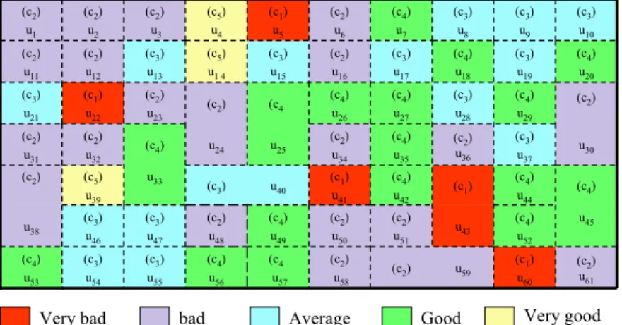
Several iterations where necessary to obtain consistent assignments. The result after the introduction of the additional information is illustrated in Figure 6. To obtain the final decision map, it needs only to regroup the neighbours spatial units which are assigned to the same category. The result after regrouping is shown in Figure 7. Note that the term "neighbours" in this example is the one of Rook where two units are neighbours only and only if they share at least one segment.

)) )) (c2) u61 (c1) u60 u59 (c2) (c2) u58 (c4 u57 (c4) u56 (c3) u55 (c3) u54 (c4) u53 u45 (c4) u52 u43 (c2) u51 (c2) u50 (c4) u49 (c2) u48 (c3) u47 (c3) u46 u38 (c₄) (c4) u44 (c₁) (c4) u42 (c1) u41 u₄₀ (c₃) u33 (c5) u39 (c2) u30 (c3) u37 (c2) u36 (c4) u35 (c2) u34 u25 u24 (c4) (c2) u32 (c2) u31 (c2) (c4) u29 (c3) u28 (c4) u27 (c4) u26 (c4 (c2) (c2) u23 (c1) u22 (c3) u21 (c₄) u₂₀ (c₃) u₁₉ (c₄) u₁₈ (c₃) u₁₇ (c₂) u₁₆ (c₃) u₁₅ (c₅) u_{1 4} (c₃) u₁₃ (c₂) u₁₂ (c₂) u₁₁ (c3) u10 (c3) u9 (c3) u8 (c4) u7 (c2) u6 (c1) u5 (c5) u4 (c2) u3 (c2) u2 (c2) u1 (c2) u61 (c1) u60 u59 (c2) (c2) u58 (c4 u57 (c4) u56 (c3) u55 (c3) u54 (c4) u53 u45 (c4) u52 u43 (c2) u51 (c2) u50 (c4) u49 (c2) u48 (c3) u47 (c3) u46 u38 (c₄) (c4) u44 (c₁) (c4) u42 (c1) u41 u₄₀ (c₃) u33 (c5) u39 (c2) u30 (c3) u37 (c2) u36 (c4) u35 (c2) u34 u25 u24 (c4) (c2) u32 (c2) u31 (c2) (c4) u29 (c3) u28 (c4) u27 (c4) u26 (c4 (c2) (c2) u23 (c1) u22 (c3) u21 (c₄) u₂₀ (c₃) u₁₉ (c₄) u₁₈ (c₃) u₁₇ (c₂) u₁₆ (c₃) u₁₅ (c₅) u_{1 4} (c₃) u₁₃ (c₂) u₁₂ (c₂) u₁₁ (c3) u10 (c3) u9 (c3) u8 (c4) u7 (c2) u6 (c1) u5 (c5) u4 (c2) u3 (c2) u2 (c2) u1

Very bad bad Average Good Very good

Figure 6 Assignment with additional information

u₂₃ u22 u18 u1 u24 u21 u17 u9 u₂₅ u₂₀ u16 u10 u8 u34 u₃₃ u₂₆ u19 u2 u32 u27 u₁₅ u11 u7 u3 u₃₅ u₃₁ u₂₈ u₁₂ u₆ u₃₀ u₂₉ u₁₄ u₁₃ u₅ u₄ u₂₃ u22 u18 u1 u24 u21 u17 u9 u₂₅ u₂₀ u16 u10 u8 u34 u₃₃ u₂₆ u19 u2 u32 u27 u₁₅ u11 u7 u3 u₃₅ u₃₁ u₂₈ u₁₂ u₆ u₃₀ u₂₉ u₁₄ u₁₃ u₅ u₄

Very bad bad Average Good Very good

Figure 7 Final decision map

4 DECISION MAP VERSUS CARTOGRAPHIC MODELLING

The objective of this section is to specify in what our approach is distinct from classical cartographic modelling. Malczewski (1999) defines cartographic modelling as ‘a procedure combining individual GIS operations to build complex models for spatial analysis’. In fact, cartographic modelling is an automatization of the manual approach introduced by McHarg (1969). The idea of McHarg is to superimpose a set of transparent-like maps representing the different factors (e.g. slope, surface drainage, soil drainage, susceptibility to erosion) considered in the problem under study. These maps are coloured according to their suitability to the decision maker(s) objectives so that, for

example, the darker the tone the higher the suitability and when these maps are superimposed, the least-cost areas are revealed by the highest tone. The GIS technology has permitted to automatize this approach and the transparent-like maps are thus replaced with digital information layers. The GIS has also permitted to apply other aggregation operators than the initial ordinal combination method of McHarg. Hopkins (1977) provides an excellent review of the additive sum-like aggregation methods early used in cartographic modelling. Then, more sophistic aggregation models driven from the multiattribute decision making (see Keeney and Raffia, 1976) have been incorporated into GIS technology (essentially raster GIS) (e.g. Carver, 1991; Jankowski, 1995). Theses aggregation models still dominate today and only few works (e.g. Martin et al., 2000; Joerin and Musy, 2001; Joerin et al., 2001) use outranking-based aggregation models (see Roy, 1996). However, these last ones are more suitable in spatial context since they permit ‘to consider both objective and subjective criteria and require fewer amount of information from the decision maker’ (Malczewski, 1999). In addition, they do not impose the transitivity of indifference and tolerate the incomparability situations. But the major (technical) drawback of outranking methods is that they are not suitable for problems implying a great or infinite number of alternatives since they require pairewise comparison across all criteria.

In Joerin (1998), the author has used a similarity indices to first subdivide the study area into homogenous zones and then these homogenous zones are considered as potential alternatives, which are classified using the ELECTRE TRI method. Subdividing the study area into zones permits to reduce significantly the number of potential alternatives to be evaluated and leads to ‘a manageable set of alternatives’ (Hall et al, 1992; Wang, 1994; Joerin et al. 2001) and outranking methods can be applied quite easily. However, this subdivision has two disadvantages (Joerin et al. 2001): (i) The resulting maps are very sensitive to spatial division; and (ii) As the number of zones (or units) is limited, the description territory becomes quite rough, resulting in a substantial loss of information. But this dilemma is solved when a homogenous zone is seen both as a physical part of the space and as a particular solution (Joerin et al. 2001).

In the light of this discussion, we think that our approach is different from classical cartographic modelling in the following points:

• Cartographic modelling is essentially an automatic procedure with no or less (generally a priori) interaction with the decision maker(s). Our generation process is largely controlled by the decision maker(s);

• Maps produced through cartographic modelling are essentially presentation-oriented ones and they are roughly used for an effective “visual” spatial decision-aid activity. Our decision maps are decision-oriented ones. In addition, the decision map is a generic tool that may serve to the generation of potential alternatives (c.f. 2.2.4) and can be extended to support collaborative and communicative spatial decision making (see §5);

• Decision map permits to explicitly represent spatial preferences of the decision maker(s). In classic cartography modelling, preferences of the

decision maker(s) are often reduced to a tabular representation, often with no explicit relation to their spatial locations;

• Aggregation is performed in early steps in the cartographic modelling process, which may lead to a substantially lost of the preferential information. In our approach, aggregation is performed in latter steps in the generation process;

• Aggregation in our approach is based on outranking relations, which we think more appropriate to deal with spatial decision making. Especially, this permits the integration of both qualitative and qualitative criteria in the problem modelling.

In addition to the fourth first points, the proposed approach differs from the Joerin’s one since it uses ELECTRE TRI to subdivide the study area into homogenous zones (Joerin (1998) uses a similarity indices). In addition, our approach differs from Joerin (1998) in that sense that homogenous zones are composed of contiguous spatial units. Indeed, in Joerin (1998) homogenous zones may be composed of non contiguous units but we think that spatial location is an important dimension in spatial decision making since two different zones with equal evaluations may seen non equivalent by the decision maker(s).

More importantly, our approach incorporates an inference model permitting to elicit the preference parameters of the decision maker(s) while respecting his/her reasoning mode, often simple, and minimizing his/her cognitive effort. As mentioned earlier, in this work we have adapted the preference inference model proposed in Mousseau and Slowinski (1998) to spatial context.

To close this section, we compare our decision map concept to the concept of interactive map tool proposed by Andrienko and Andrienko (1999) and Jankowski et al. (2001) and the concept of decision map introduced by Lotov,

et al. (1997). The basic idea of Lotov’s decision map is to use map-based

structures in order to provide an on-line visualization of the decision space, enabling the decision maker(s) to appreciate visually how the feasibility frontiers and criterion trade-offs evolve when one or several decision parameters change. So, Lotov’s decision map is by construction different from our decision map (but should we change the name!). Concerning interactivity and map-centred exploratory analysis tools, we think that they are complementary tools to our decision map. In fact, interactivity will undoubtedly add value to our decision map and will provide a more convivial communication support and permit a better what-if analysis.

5 DECISION MAP FOR GROUPS

In this section, we suppose that K groups or individuals are involved in the spatial decision making process. Such a group or an individual could be specialist in technical domains (expert knowledge) connected to urban planning or be representatives of interests and objectives of local communities (experiential knowledge). The objective is to generate a composite decision map that summarizes the preferences and objectives of all the participants in a collaborative and communicative decision process.

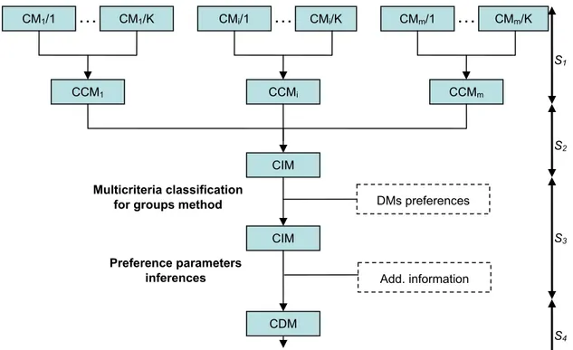
Inspiring from the work of Dias and Clímaco (2000), we may distinguish two ways for generating the composite decision map, along with the level where the global aggregation is performed. In the first approach, aggregation is performed at the input level, i.e., at the level of criteria maps definition (Figure 8). Operationally, this approach starts by the definition of composite criteria maps for all the evaluation criteria. Then, these composite criterion maps are aggregated so that to obtain a composite intermediate map. Then, the second step of the process is similar to the one described in section 2.2 but here a multicriteria classification method for groups is used. At this level, preference parameters of all the groups should be considered. In the third step, the inference model is adapted to take into account additional information provided by the different involved groups. In the last step, the generated composite decision map is enhanced so that to support “visual” spatial decision making for groups.

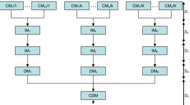
In the second approach global aggregation is performed at the output level (Figure 9). Operationally, each group first generates an individual decision map as in 2.2. Then, these obtained individual maps are superimposed and an aggregation operator is applied to generate a composite decision map.

…

…

…

for groups method

S3

CIM

Preference parameters

inferences Add. information

CDM

S4

Presentation + (“visual”) spatial decision making for groups

•CMi /k: criterion map for criterion gi and group k •CIM : composite intermediate map

•CCMi : composite criterion map for criterion gi •CDM: composite decision map

•Sj: step j

Figure 8 Composite decision map generation: Approach 1

Clearly, the first approach is more convenient since the groups or individuals are collectively involved during all the phases of the generation procedure, from criterion maps definition to the composite decision map generation.

Furthermore, the first approach is more appropriate for situations with no strong conflict among the groups. However, technically this approach is more complex to implement and may require more time than the second approach. In turn, the second approach is more flexible since different groups may consider different evaluation criteria. Then, it is appropriate for collaborative and communicative processes directed to generate consensual directions of urban and territorial policies. In addition, this second approach seems to be more appropriate in situations of strong conflict.

…

…

…

Presentation + (“visual”) spatial decision making for groups

•CMi/k : criterion map for criterion gi and group k •DMk : decision map for group k

•IMk : intermediate map for group k •CDM: composite decision map for group k

•Sj: step j

Figure 9 Composite decision map generation: Approach 2

To conclude this section, we think that the decision map concept is a powerful tool for collaborative and communicative spatial decision making since:

• The decision map permits to include, by construction, the preference of the entire participants;

• The decision map permits to visually and spatially represent the preferences of all the participants. It may be superimposed with other layers representing the physical environment for a better appreciation. Thus it constitutes a base for negotiation/consultation activities and the derived decision will normally be accepted;

• When decision map is enriched with spatial data exploration tools and an enhanced interactivity, it permits an effective what-if analysis and a better and constructive dialogue between all the participants;

• We think that the construction of decision map for groups permits to implement a constructive spatial decision making approach rather than a descriptive one as in classical cartographic modelling.

6 CONCLUSION

In this paper we have introduced the concept of decision map. When it is effectively integrated into GIS, the decision map permits to avoid, fully or partially, several ones of the limitations of large scales models enumerated in the introduction. The concept of decision map is a generic tool that may be used for several purposes (e.g. generation of potential alternatives, communication and participation). In this paper, we have focalised on the general aspects of the decision map. We have also showed how the decision map concept can be extended to support collaborative and communicative spatial decision making in urban planning.

REFERENCES

Andrienko, G., and Andrienko, N. (1999) Interactive maps for visual data exploration. International Journal of Geographical Information Science, Vol. 13, No. 4, 355-374.

Batty, M. (1994) A chronicle of scientific planning: The Anglo-American modeling experience. Journal of the American Planning Association, Vol. 60, No. 7, 7-16. Braux, C. (1996) Cartographie multicritère: Guide méthodologique. Technical Report No. R 39146, BRGM, France.

Chakhar, S., and Mousseau, V. (2004) Towards a typology of spatial decision problems. Annales du LAMSADE, No. 2, 125-154.

Carver, S. (1991) Integrating multicriteria evaluation with GIS. International Journal of Geographical Information Systems, Vol. 5, No. 3, 321-339.

Dias, L.C., and Clímaco, J.N. (2000) ELECTRE TRI for groups with imprecise information on parameter values. Group Decision and Negotiation, Vol. 9, No. 5, 355-377.

Dias, L.C., and Mousseau, V. (2005) IRIS: a DSS for multiple criteria sorting problems. Journal of Multi-Criteria Decision Analysis, Vol. 12, No. 1,1-14.

Hall, G.B., Wang, F., and Subaryono (1992) Comparison of boolean and fuzzy classification methods in land suitability analysis by using geographical information systems. Enviornnment and Planning A, Vol. 24, 497-516.

Healey, P. (1992) A planner's day: Knowledge and action in communicative practice. Journal of the American Planning Association, Vol. 58, 9-20.

Healey, P. (1997) Collaborative planning. Macmillan, London, UK.

Hopkins, L.D. (1977) Methods for generating land suitability maps: A comparative evaluation. Journal of the American Institute of Planners, Vol. 43, No. 4, 386-400. Innes, J. (1995) Planning theory's emerging paradigm: Communicative action and interactive practice. Journal of Planning Education and Research, Vol. 14, No. 3, 183-190.

Jankowski, P. (1995) Integrating geographical information systems and multiple criteria decision-making methods. International Journal of Geographical Information Systems, Vol. 9, No. 3, 251-273.

Jankowski, P., Andrienko, N., and Andrienko, G. (2001) Map-centered exploratory approach to multiple criteria spatial decision making. International Journal of Geographical Information Science, Vol. 15, No. 2, 101-127.

Joerin, F. (1998) Décider sur le territoire: Proposition d’une approche par l’utilisation de SIG et de méthods multicritère. PhDThesis No. 1755, EPFL, Switzerland.

Joerin, F. and Musy, A. (2000) Land management with GIS and multicriteria analysis. International Transactions on Operational Research, Vol. 7, 67-78.

Joerin, F., Thériault M., and Musy A. (2001) Using GIS and outranking multicriteria analysis for land-use suitability assessment. International Journal of Geographical Information Science, Vol. 15, No. 2, 153-174.

Keeney, R., Raffia, H. (1976) Decision with multiple objectives: Preferences and value tradeoffs. John Wiley and Sons, New York.

Lee, D.B. (1973) Requiem for large-scale models. Journal of American Institute of Planners Vol. 39, 163-178.

Lotov, A.V., Bushenkov, V.A., Chernov, A.V., Gusev, D.V., and Kamenev, G.K. (1997) Internet, GIS, and interactive decision map. Journal of Geographical Information and Decision Analysis, Vol. 1, No. 2, 118-149.

MacHarg, I.L. (1969) Design with nature. Natural History Press, NewYork.

Malczewski, J. (1999) GIS and mutlicriteria decision analysis. John Wiley & Sons, NewYork.

Martin, N., St-Onge, B. and Waaub, J.-P. (2000) An integrated decision aid system for the development of Saint-Charles River's alluvial plain, Québec, Canada. International Journal of Environmental Pollution, Vol. 12, No. 2/3, 264-279.

Mousseau, V. (2005) A general framework for constructive learning preference elicitation in multiple criteria decision aid. Cahiers du LAMSADE, No. 223, University Paris Dauphine.

Mousseau, V., and Slowinski, R. (1998) Inferring an ELECTRE TRI model from assignment examples. Journl of Global Optimization, Vol.12, No. 2, 157-174. Roy, B. (1996) Multicriteria methodology for decision aiding. Kluwer Academic Publishers, Dordrecht.

Wang, F. (1994) The use of artificial neural networks in geographical information system for agricultural land-suitability assessment. Environment and Planning A, Vol. 26, 265-284.

Yu, W. (1992) ELECTRE TRI. Aspects méthodologiques et guide d’utilisation. Document du LAMSADE, No. 74, University Paris Dauphine.