The Determinants of the Time to Efficiency in Options
Markets : A Survival Analysis Approach
L
AURENTD
EVILLE∗F
ABRICER
IVA†November 2004
Abstract
This paper examines the determinants of the time it takes for an index options market to be brought back to efficiency after put-call parity deviations, using intraday transactions data from the French CAC 40 index options over the August 2000 – July 2001 period. We address this issue through survival analysis which allows us to characterize how differences in market conditions influence the expected time before the market reaches the no-arbitrage relationship. We find that moneyness, maturity, trading volume as well as trade imbalances in call and put options, and volatility are important in understanding why some arbitrage opportunities disappear faster than others. After controlling for differences in the trading environnement, we find evidence of a negative relationship between the existence of ETFs on the index and the time to efficiency.
KEY WORDS: Index Options, Market efficiency, Survival Analysis, Exchange Traded Funds.
JEL CLASSIFICATION: C41, G13, G14.
∗CNRS; CEREG (UMR 7088); Paris Dauphine University; Place du Maréchal de Lattre de Tassigny;
75775 Paris Cedex 16, France; Tel.: +33 (0)1 44 05 45 36; Fax: +33 (0)1 44 05 40 23; e-mail: [email protected]
†CEREG (UMR 7088); Paris Dauphine University; Place du Maréchal de Lattre de Tassigny; 75775 Paris
Cedex 16, France; Tel.: +33 (0)1 44 05 49 88; Fax: +33 (0)1 44 05 40 23; e-mail: [email protected]. The insightful comments and suggestions of Bruno Biais, Hazem Daouk, Thierry Foucault and seminar participants at the Toulouse Master in Finance Inaugural Conference, the Europlace Institute of Finance November 2004 Research Days, and the French Finance Association 2004 Annual Meeting are gratefully acknowledged.
1
Introduction
Researches on options markets efficiency based on arbitrage relationships commonly agree that these relationships hold on average. However, whether it be on US1 or European markets2, distortions are observed, whatever the quality of the data, the kind of underlying asset and how carefully the computations of profits are led. The most striking evidence is provided by Kamara and Miller (1995) on the S&P 500 options contract from May 1986 through May 1989. They document frequent put-call parity violations, even with a European contract, prices matched within a minute and accounting for transaction costs and dividends. Hence, there are times when options markets appear to be incompatible with no arbitrage prices and therefore with efficiency.
However, as pointed out in Chordia, Roll and Subrahmanyam (2004), “efficiency does not just congeal from spontaneous combustion” but is a process that depends on individual actions and, as a result, takes time. Efficient is the market where, after a distortion has been identified, prices revert rapidly enough to stop subsequent arbitrage trades. Efficiency will depend on the traders’ ability to realize riskless abnormal profits given the information that the market prices are not compatible with no-arbitrage at a given time. On options markets, two principal ways have been followed since now to assess this aspect of efficiency: one based on the computations of accessible ex ante profits and the other based on the identification of the determinants of the immediate (ex post) profits.
Arbitrage-oriented transactions cannot be immediate after an opportunity has been identi-fied. The prices a trader can get may differ from the ones he observed. The index level may move and the market makers could have adjusted their quotes both to account for this variation and, if the case need be, to protect themselves from arbitrage trades. Hence, accessible (ex ante) profits may be different from the identified (ex post) opportunities and accurate efficiency tests have to be based on the level of such ex ante profits. The classical way of deriving such ex ante profits (see Galai, 1977) is to measure the profits an arbitrageur can earn when being im-posed an arbitrary “no trade” period. Kamara and Miller (1995), for the S&P 500 index options,
1Put-call parity empirical studies include Gould and Galai (1974) on OTC options, Klemkoski and Resnick
(1979, 1980) on stock options traded on the CBOE, Evnine and Rudd (1985) , Chance (1987), Finucane (1991) and Wagner, Ellis and Dubofsky (1996) on S&P 100, and Kamara and Miller (1995), Ackert and Tian (2001) and Bharadwaj and Wiggins (2001) on S&P 500. The latter two studies test other arbitrage relationships, such as the box-spread, also tested by Billingsley and Chance (1985), Chance (1987) and Ackert and Tian (1998).
2For empirical tests of arbitrage relationships on European index contracts, see Puttonen (1993) for the Finnish
market, Chesney, Gibson and Loubergé (1995) for the Swiss market, Cavallo and Mammola (2000) and Cassese and Guidolin (2001) for the Italian market, and Capelle-Blancard and Chaudhury (2001) and Deville (2004) for the French market.
Mittnik and Rieken (2000) for the German DAX 30 index options and Deville (2004) for the French CAC 40 index options show that ex ante profits decrease with the length of the no-trade window. Hence, market prices adjust after a deviation occurred but not instantaneously and arbitrage opportunities persist for a while. Despite the introduction of a time-dimension in effi-ciency tests, ex ante tests still focus on the level of profits and are by no means truly dynamical although efficiency is.
To explain why apparent profits may appear on the S&P 500 index options market, Kamara and Miller (1995) regress the level of ex post put-call parity arbitrage profits identified at the market close on explanatory variables. Using a bootstrapped Tobit regression which allows them to appropriately handle the censored observations that are compatible with no-arbitrage, they show that the profit can be explained by liquidity risk factors. Hence, rather than reflecting inefficiency, ex post profits appear to be premia for the liquidity risk faced by investors who may engage in subsequent arbitrage trades. Following the same methodology, Ackert and Tian (2001) roughly obtain the same results for the various arbitrage relationships they test for the S&P 500 index options.
The profits available on the basis of put-call parity arbitrages tend to decrease as time goes by. Liquidity has been found to be important in explaining the size of the violations. However, existing studies are silent regarding why and how prices go back to efficiency levels. Our study precisely aims at understanding the process by which prices revert to levels compatible with no-arbitrage. This work is closely related to Deville (2004) who measures the options market (in)efficiency as the time during which prices remain incompatible with the no-arbitrage levels implied by the put-call parity relationship. This measure is truly dynamic and uses the whole information set available with intraday data. Every index level and transaction price subsequent to the identification of a distortion is actually considered. Since then, this measure should prove most appropriate in identifying the determinants of efficiency or, in other words, in studying how efficiency emerges in the options markets.
Since our work focuses on durations rather than profits, we resort to a particular statistical technique called survival analysis, which allows to model and analyze lifetime data. Our pop-ulation is the set of matched pairs of call and put options transactions that are not compatible with put-call parity. We consider an observation as ‘alive’ as long as the profit resulting from the construction of the arbitrage portfolio remains positive. It is considered as ‘dead’ as soon as the built portfolio leads to a negative or zero profit. Survival analysis also proves useful to correctly accommodate an important feature of time to efficiency: censored observations i.e. matched pairs that still exhibit a positive profit at the market close.
for the French CAC 40 index options from August 1, 2000 through July 31, 2001. This period surrounds January 21, 2001, the launching date of the ETF that replicates the CAC 40 index, which makes it possible to study the incidence of this new asset on the efficiency process. By introducing explanatory variables in the survival analysis we are able to control for the impact of the market activity on the duration of inefficiencies. The probability that an arbitrage opportunity dies conditionally to the fact that is has lived since is found to be decreasing with time: the more a deviation lasts, the more it has chance to last one more instant. Hence, a deviation that is not quickly brought back to efficiency may last for a long time, and this may illustrate the fact that some opportunities are exploited by arbitrageurs while some others are not worth the trouble. We find that the time to efficiency is negatively linked with several explanatory variables such as the activity on the options market, the volatility on the underlying asset and the possibility to trade the CAC 40 index through ETFs. We also document that differences in option characteristics lead to significant changes in the probability for an arbitrage opportunity to survive over a given time interval.
The remainder of this paper is organized as follows. Section 2 details the time to efficiency computations and reviews the survival analysis methodology. Section 3 describes the data. Sec-tion 4 presents the empirical results of our analysis of the determinants of the time to efficiency. Section 5 concludes.
2
General methodology
In our analysis, prices are considered efficient as soon as they are compatible with the put-call parity relationship. Though restricting our analysis to times when a pair of put and call options transactions on the same series have been matched, this definition makes it possible to identify the forces driving the prices back to efficiency without resorting to any option pricing model. We briefly present the well-known put-call parity relationship and our a measure of efficiency based on the time it takes for a distortion to disappear, namely the time to efficiency. Then, we review the econometric tool we employ to isolate variables that impact this time, i.e. the survival analysis.
2.1
Put-call parity relationship and arbitrage profits
The notation used in the discussion is as follows: Ct, European call premium at time t,
K, strike price, It, index value,
τ , time to maturity, r, risk-free interest rate,
D, present value of dividends paid from the transaction date until expiration, expressed in index points.
Under no-arbitrage, whenever put and call options having the same characteristics exist, their premia must satisfy the put-call parity relationship3(PCP):
Ct− Pt = It+ D − Ke−rτ (1)
If equation (1) does not hold, the call option is either under- or over-valued with respect to the put option and an arbitrage portfolio might be built by taking opposite positions in the ‘real’ and the synthetic call option. These strategies are called ‘long hedge’ and ‘short hedge’, respectively, dependent on the position that is held on the underlying asset. If dividends are to be paid during the life of the options, the initial positive flow generated by these two strategies, denoted πLH and πSH, respectively, are equal to:
πLH = Ct− Pt− It+ D + Ke−rτ (2)
and:
πSH = Pt− Ct+ It− D − Ke−rτ (3)
These initial flows represent the ex post arbitrage profit – that may be obtained from the con-struction at time t of the portfolios. Both portfolios are to be held until expiration, at which time in-the-money options will be exercised and the index position cleared, leading to a zero terminal payoff.
Classical efficiency tests are based on the level of initial profits that can eventually be earned from the exploitation of identified opportunities. The time-dimension is lacking in this measure although, as emphasized in the introduction, efficiency is a dynamic process. In this paper, we prefer the use of a measure that relies on the duration of inefficiencies rather than on the identified level of profits.
3Put-call parity was initially formalized by Stoll (1969) for at-the-money options and extended for non-payout
2.2
TTE as a measure of market (in)efficiency
The measure of informational efficiency of derivatives markets we use in this paper, namely the time to efficiency (hereafter TTE), has been developed in Deville (2004). Basically, it consists in measuring how long it takes for the market prices to revert to no-arbitrage values, once a deviation has been identified.
The way TTE is computed is the following. We first match pairs of synchronous transactions of calls and puts having the same characteristics. We compute the initial (ex post) arbitrage profit using equations (2) and (3) as a function of the prices Pt, Ct and It that prevail at the
pairing time, t. If πLH (πSH) is positive, the pair is classified as a long hedge (short hedge)
deviation to put-call parity4. Then, each time a new market value is recorded for one of the
three components of the arbitrage portfolio (put, call and index), its price is updated5. The profit
resulting from the construction of the arbitrage portfolio at this time is then computed with this new set of prices using equations (2) and (3) for the long hedge and short hedge deviations, respectively. The updating process stops as soon as the profit becomes zero or negative, as prices are then compatible with no arbitrage. The time to efficiency is the time it takes for the arbitrage profit to go zero prior to the market close, if ever.
As an example, consider a deviation occurring at time t with πLH > 0. To compute the
TTE, we look for the first subsequent modification in the value of either the put, the call or the index. Denote t + 1 the time when a modification first occurs. If the only modification recorded at time t + 1 is a variation in the index value, profit is computed at time t + 1 with the set of prices Pt, Ctand It+1as:
Ct− Pt− It+1+ D + Ke−rτ
A negative or null value for the profit stops the computations and the time to efficiency equals the time elapsed between t and t + 1. If the profit remains positive, we look for the next modification in the value of at least one of the three instruments. Denote t + 2 the time when
4Without transaction costs, π
LH = −πSHand every matching deviates from put-call parity, either on the long
hedge side or on the short hedge side. Transaction costs create a bandwidth within which prices can fluctuate without inducing any profitable arbitrage opportunity. They are not accounted for in this study since, as shown in Deville (2004), their effect is only to reduce the number of observed deviations without affecting the distribution of TTEs or the general trends towards efficiency values.
5It happens that multiple transactions for options having the same characteristics are recorded in the same
minute, with different transaction prices. In this case, we choose to keep the premium that leads to the smallest profit. In the case of long hedges (short hedges), we therefore use the most (less) expensive calls and the less (most) expensive puts. As a result, we obtain a lower bound for the TTE. We have also estimated an upper bound by deriving the profit with the premium that leads to the highest value. Results, available on request, are only marginally modified since transactions, when recorded simultaneously, rarely present significantly different premia.
this second modification occurs. If the modifications recorded between t + 1 and t + 2 are variations in the index value and in the call price, profit is computed at time t + 2 with the set of prices Pt, Ct+2and It+2as:
Ct+2− Pt− It+2+ D + Ke−rτ
The process goes on in the case of a positive value and stops in the case of negative or null value, with the time to efficiency being equal to the time (in seconds) elapsed between t and t + 2.
It is important to note that the time elapsed between two subsequent events is not a constant as it depends on the frequency of dissemination of the index values and the transaction times of calls and puts of the same series. Another important feature of the TTE is that its computation relaxes the synchronism constraint initially imposed on the prices of the instruments included in the arbitrage portfolio. Implicitly, this supposes that there is no price staleness. However, it is also the case for the classical ex ante tests of options markets efficiency in which the prices considered for the computation are the first one observed for each instrument once the execution delay has passed, without any constraint on synchronism.
The set of options transactions prices and index values recorded before the market close do not necessarily induce a return to efficient prices. After the close, no information regarding the index value or options prices is disseminated until the market opening on the following day. Rather than using opening prices to go on with TTE computation procedure, we stop it at the close. If the profit remains always positive throughout the remainder of the trading day, no TTE is derived and we compute the time elapsed between the identification of the deviation and the market close. We refer to this time as the time to censoring. The information we retain is that prices were still inefficient after this duration. Hence, the distribution of TTEs is right-censored. However, this doesn’t mean that we have to drop such observations out of our sample since censorship can be properly handled with survival analysis.
2.3
A brief review of survival analysis
In this section, we develop an econometric model which aims at explaining the determinants of the time it takes for an arbitrage opportunity to disappear. We employ a statistical tool called survival analysis, a commonly used technique in the area of biostatistics, but whose applications in financial research are sparse6. Survival analysis is particularly well-suited in our context since
6Notable exceptions are the studies by Lo, MacKinlay and Zhang (2002) and Bisière and Kamionka (2000).
we want to estimate the impact of market conditions for the survival of censored TTEs.
2.3.1 Basic quantities
The most important quantity to describe time-to-event data is the survival function, which gives the probability of an individual (in our case, an arbitrage opportunity) surviving beyond time t. It is defined as:
S(t) = P r(T > t) (4)
When T is a continuous random variable, the survival function is given by:
S(t) =
Z ∞
t
f (x)dx = 1 − F (t) (5)
where f (·) denotes the probability density function of T , F (·) its cumulated density function, and thus
f (t) = −dS(t)
dt (6)
A quantity that is closely related to the survival function is the hazard function, which gives the probability that an event that has lasted up to time t will terminate in the interval [t, t + ∆t]. Its formal definition is given by:
h(t) = lim
∆t→0
P r(t ≤ T < t + ∆t | T ≥ t)
∆t (7)
and for continuous variables,
h(t) = f (t) S(t) = −
d log[S(t)]
dt (8)
Integrating the hazard function over [0, t] yields the integrated or cumulated hazard function
Λ(t) = Z t
0
h(x)dx = − log[S(t)] (9)
whose main usage arises when one has to perform graphical checks of model adequacy (see section 4.3).
2.3.2 Estimation procedure
Our approach to estimating the survivor function falls into the parametric case. Within this framework, a parametric form is assumed for the distribution f (.) of failure times (in our case times to efficiency) which allows direct computation of the likelihood function for the data. Notice that for some of our observations – namely the ones for which the arbitrage profit remains positive up to the market close – the only available observation is the time to censoring, which gives a lower bound estimate for the actual time to efficiency. This is not a concern however since survival analysis allows to accommodate such (right-) censored observations in an efficient way.
The general procedure is the following. Uncensored observations provide information on the probability that an arbitrage opportunity has survived to its associated time to efficiency, which is equal to the density function of T at that time (denoted Ti). For right-censored
obser-vations, the appropriate quantity is the survival function as the only thing we know about the true time is that it is greater than the censoring time (denoted Ci).
Under the assumption that the censoring time Ci is independent from the true time Ti, we
obtain the likelihood function for our sample as7:
L =
n
Y
i=1
f (ti)δiS(ti)(1−δi) (10)
where ti = min(Ti, Ci), and δi = 1{Ti≤Ci} is a dummy variable which takes value one for uncensored observations and 0 otherwise.
2.3.3 The Weibull distribution
So far, we have not set any structure on the distribution T is drawn from. Among the different alternatives, we decided to focus on the Weibull distribution as it is both fairly general and mathematically tractable.
The Weibull distribution is a two-parameter distribution whose p.d.f. is:
fW(t) = αλtα−1exp
¡
−λtα¢, t > 0 (11)
7Differently stated in our case, time to censoring (i.e. time to close) provides no information about what would
and the associated survival function is:
SW(t) = exp
¡
−λtα¢ (12)
with α > 0 the shape parameter and λ > 0 the scale parameter.
From the definition of the hazard function in the continuous case, the hazard function when T follows a Weibull distribution comes to be:
hW(t) = αλtα−1 (13)
so that the Weibull distribution can accommodate increasing (α > 1), constant (α = 1) or decreasing (α < 1) hazard.
2.3.4 Including covariates
As we are interested in studying the effects of the trading environment on the efficiency of options markets, our approach needs to incorporate explanatory variables time to efficiency shall depend on into the likelihood function. The most common way to proceed assumes a linear relationship between the log of survival time and the covariates (explanatory variables) values, namely:
Y = ln(T ) = µ + γ0Z + σU (14)
where γ0 = (γ1, . . . , γp) is a vector of regression coefficients and U is the error distribution. Such an approach is called accelerated failure time (AFT) as the effect of the explanatory vari-ables in the original time scale is to accelerate (decelerate) time by a constant factor exp(−γ0Z) when γ is negative (positive).
Computations for the p.d.f. of Y = ln T when T follows a Weibull distribution yield:
fY(y) = αλ exp ³ αt − λeαt´, −∞ < y < +∞ (15) Setting ( λ = exp(−µ/σ) α = 1/σ (16)
fY(y) is found to be:
fY(y) = 1 σ exp à t − µ σ − exp à t − µ σ !! , −∞ < y < +∞ (17)
with an associated survival function: SY(y) = exp µ − exp · (y − µ)/σ ¸¶ (18)
From (17), it comes that the p.d.f. of the error term U = (Y − µ)/σ in the Weibull case is given by:
fU(u) = exp
¡
u − eu¢ (19)
which is the p.d.f. of a standard extreme value distribution. Direct computations yield the corresponding survival function:
SU(u) = exp(− exp(u)) (20)
Using (10) and plugging covariates, the likelihood function for right-censored data when T follows a Weibull is given by:
L = n Y i=1 £ fY(yi) ¤δi£ SY(yi) ¤δi = n Y i=1 " 1 σfU Ã yi− µ − γ0Z σ !#δi" SU Ã yi− µ − γ0Z σ !#δi (21)
where fY(y), SY(y), fU(u) and SU(u) are given in (17) – (20). This function will form the
basis of our estimation procedure.
3
The data
We empirically investigate the determinants of the TTE for the CAC 40 index options contract for the 12-month period from August 2000 to July 2001. Derivative contracts on CAC 40 are the most traded ones on the Marché des Options Négociables de Paris (MONEP), the French market for equity and index derivatives8. The efficiency of this contract constitutes a benchmark for the MONEP efficiency. We first describe the specifications of options and ETF contracts on CAC 40 index and then detail our data set of TTEs.
8Since the acquisition of LIFFE (the London International Financial Futures and Options Exchange) by
3.1
CAC 40 index options and ETFs contracts
9The CAC 40 index consists of 40 stocks selected from the most active and representative among the various economic sectors quoted on the Paris “Premier Marché”. Its value is calculated con-tinuously as the weighted average market capitalization of the 40 stock prices, and is dissemi-nated every 30 seconds by Euronext Paris. The index is managed by an independent committee, the “Conseil Scientifique des Indices”, which adapts the index to reflect changes in the market or in the market capitalization of the constituent stocks.
The CAC 40 index option (PXL ticker) is the MONEP most active contract. Over year 2000, it accounts for one third of the total open interest and one half of the number of trades on the French options market. From August 2000 through July 2001 a monthly average volume of more than 7 millions contracts were traded, which represent 1 billion Euros premium. On the MONEP, orders are send to a Central Order Book by members and executed according to price/time priority. Nevertheless, committed market-makers continuously compete for the order flow. Market makers have an obligation to maintain a permanent bid-ask spread for option series near the money and must publicly reply to any investor’s price demand within 30 seconds by sending bid and offers prices binding for two minutes. Transactions on the MONEP are carried out by matching buy and sell orders. Orders offering the best execution conditions are given priority, with priority for orders at the same price determined by their time-stamp in the central order book. As it is the case for stock trading on Euronext Paris, after a call-auction, the quote is continuously ensured from 9.02 a.m. to 5.30 p.m. on the automated system NSC until the closing call-auction at 5.35 p.m.10.
The size of PXL contracts is equal to the value of the CAC 40 index multiplied by one Euro and the tick size is 0.1 index point. This contract is cash-settled11and is exclusively composed of
European-style options. Trading covers eight rolling open maturities: three spot months, three quarterly maturities and two half-yearly maturities. The same expiration months are opened for the futures contract on the CAC 40 index, which is also traded on the MONEP. Strike prices are set at standard intervals of 50, 100 or 200 points dependent on the expiration date. The series opened to trading are not necessarily the same for call and put options. At every moment in
9Informations given in this subsection are about the sample period and may have changed since. In particular,
for contracts expiring after September 2004, expiration date has moved from the last trading day of the expiration month to the third Friday of the expiration month and fourteen instead of eight maturities are traded.
10On 23 April 2001, Euronext implemented a common market model in its three constituent market places,
Paris, Amsterdam and Brussels. The continuous trading period now ranges from 9:00 for the open to 5.25 p.m. for the close, followed by a closing call auction (fixing) at 5.30 p.m.
11The settlement value is equal to the mean of all index values calculated and disseminated between 3.40 p.m.
time, at least three strike prices are listed: one “at the money” and two “out of the money”. New series are created dependent on the price changes of the CAC 40 index.
CAC 40 Master Unit, the first ETF traded in Paris since January 22, 2001, is aimed at replicating price and performance of the CAC 40 index. Its initial value was 1/100th of the
index value. Dividends equal to the total amount of dividends accumulated by the fund minus management expenses of 0.30% are paid on an annual basis. ETFs are traded on two parallel markets, each governed by its own rules. The primary market is the issuing market, where the creation and redemption of parts of the fund can be carried out. Meanwhile, ETFs listed on Euronext can be traded on its secondary market, NextTrack.
As an open-ended fund, the assets under management (which Net Asset Value is dissemi-nated once a day) may vary over time, through the creation and redemption of full multiples of 50,000 tradable shares of the fund, which roughly represent 500 times the CAC 40 index euro-denominated value. As an example, the capital managed by the CAC 40 Master Unit issuer, namely Lyxor Asset Management, was 765, 655 thousand Euros (corresponding to 17, 338, 211 shares) after one year and 1, 038, 333 thousand Euros (34, 750, 111 shares) after two years. NextTrack, the secondary market for the CAC 40 Master Unit, is almost organized as Euronext Paris Premier Marché. ETFs are traded continuously through an electronic order book accessi-ble to both issuers and investors from 9.05 a.m. to 5.25 p.m. A closing auction takes place at 5.35 p.m. One difference from the usual French stock market trading is the mandatory presence of committed market participants that provide liquidity by continuously posting quotes in the order book for a minimum order size. They have to maintain a maximum spread of 0.40% up to five million Euros for the CAC 40 Master Unit.
3.2
Data and TTE results
The intraday transactions data on the PXL contract have been extracted from the Euronext Paris Market Database from August 2000 to July 2001. For the 78, 887 call and 92, 059 put options recorded transactions, this database reports the strike price and the expiration month, as well as time-stamped informations such as the premium and the number of traded contracts. Dividends on French stocks are usually paid on an annual basis with a high concentration in May and June. Discrete dividends have been extracted from Thomson Financial Datastream and expressed in terms of CAC 40 index points on a daily basis. For each matching, the present value of the dividends paid between the trade and the expiration date is calculated using Euribor as a proxy for the risk-free interest rate. The source for one week to one year Euribor rates is Thomson Financial Datastream. For each matching, we use a linear interpolation of the nearest Euribor
rates around the time to maturity of the options contracts.
A matching pair is selected each time we observe a call and a put having the same exact characteristics (strike price and expiration month) traded within a one minute interval. Each pairing is associated with the index value prevailing at the same time12, extracted from Euronext
Database. Thus, we avoid asynchronous bias that can lead to an overestimation of market efficiency. Options with less than two days and more than one year to expiration as well as trades recorded with a premium less than 2 Euros are excluded from the sample. Such options account for 7.55% of the 170, 946 recorded transactions. This leads to a final sample of 4, 279 matching pairs, out of which 1, 733 have been recorded before the introduction of the ETF and
2, 546 afterwards.
[Table 1 about here.]
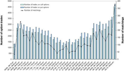
Since we require that call and put transactions occur within a one-minute interval, market efficiency is actually tested at specific points in time. The matching procedure might produce numerous pairings when market activity is high and no observation at all when it is low. One question that naturally arises is whether our sample of matchings is representative of the whole market activity. As reported in the upper part of Table 1, almost 80% of the pairings correspond to options series that are less than one month to maturity, and the number of pairings decreases with the time to maturity. This is consistent with the trading activity on both put and call options series on the MONEP, which is highly concentrated on the nearby maturity. Figure 1 depicts the intraday activity of both put and call options transactions for fifteen-minute intervals. Trading activity slowly decreases from the market opening until 2.00 p.m. and then rises throughout the afternoon to reach its maximum at the close. The distribution of pairings, represented on the same figure, follows the same intraday trend. The number of matched pairs increases when the activity is higher, but still, a significant number of matching pairs is recorded in the middle of the day, when the activity is at its lowest. Overall, our sample of matching pairs is thus representative of the market activity in call and put options, and our results may offer a fair view of the PXL contracts efficiency.
[Figure 1 about here.]
The bottom of Table 1 reports the observed times to efficiency (sample B) and times to censoring (sample A) both for the full sample (4,279 put-call parity matching pairs), and for
12When the pairing is not synchronous, we match it with the index value prevailing at the time of the second
transaction. It is consistent with arbitrageurs that would monitor the options market and try to build the arbitrage portfolio only once an opportunity has been identified.
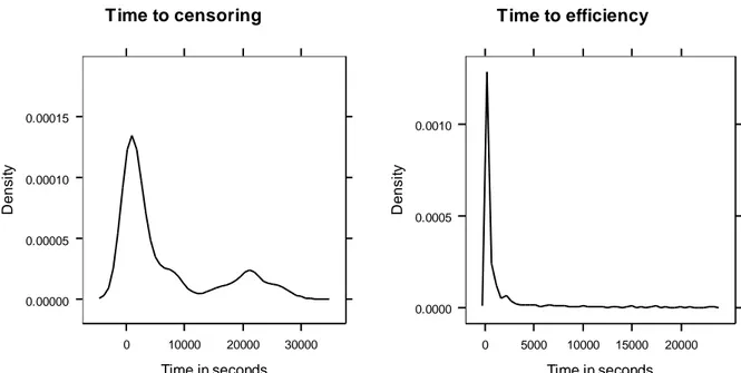
the observations observed before (1,733 matching pairs) and after (2,546 matching pairs) the introduction of the ETF on the CAC 40 index. One important feature of our computations is that 432 matching pairs (10.10% of the full sample) are censored observations of TTEs since they do not revert to efficiency-compatible levels before the market close. The average time to censoring is 106.27 minutes whereas its median is 31.83 minutes. As the distribution of times to censoring shown in figure 2 underlines it, this sample is constituted by a low proportion of matching pairs identified early in the trading day with prices remaining inefficient for a long period until the market close. A higher proportion of the matching pairs which do not return to efficiency are observed within the last 30 minutes of the trading day. This was expected since there is both a shorter remaining time to conclude trades and index moves are much more limited than it is the case for earlier matching pairs. Time to censoring dramatically decreases for the period following the introduction of the ETF. Hence, if their proportion remains of the order of 10% of the full sample, censored matching pairs are much closer to the end of the trading day once the ETF is available, less matching pairs remaining incompatible with efficient prices for long durations.
Sample B gathers the 3,847 matching pairs that revert to efficient prices before the end of the trading day. On average, one transaction is enough to exhaust the arbitrage profit. Positive profits may nonetheless be obtained until 19.22 minutes after the identification of the arbitrage opportunity, on average. However, it must be noted that the distribution of TTEs, depicted in the right part of figure 2, has a very fat left tail and is right-skewed. This sample appears to be constituted by a high proportion of short TTEs and a small proportion of very long TTEs. Although, overall, the median TTE is 3.60 minutes only, it significantly decreases from 4.90 minutes before the introduction of ETFs to 3.32 after. Hence, the possibility of trading the CAC 40 index through ETFs appears to enhance the options market efficiency. Most of the opportunities disappear within five minutes. Still, it takes more than one hour for prices to be brought back to levels compatible with no arbitrage for 10.91% of the matching pairs that exhibit a return to efficiency and the maximum TTE is greater than six hours whether it be before or after the introduction of the ETF.
[Figure 2 about here.]
Overall, the market looks efficient in the sense that prices do not remain incompatible with no-arbitrage for long but there appears to be a high degree of variability in the way prices revert to efficiency-compatible level. Some opportunities disappear very rapidly whereas others remain for hours incompatible with no arbitrage. We study why it is so in the next section.
4
Empirical results
This section is devoted to the empirical analysis of the determinants of the time to efficiency for the data described in the previous section using the survival approach reviewed in section 2.3. In section 4.1, we detail the explanatory variables we use. Section 4.2 presents the parameter estimates. We check for the adequacy of our parametrization in section 4.3 and we discuss the implications of our estimates in section 4.4. We end the presentation of the empirical results with additional analysis in section 4.5.
4.1
Explanatory variables
To understand the reasons why some arbitrage opportunities disappear faster (if ever) than oth-ers, we use several explanatory variables which aim at capturing the trading environment that prevails at the time we match options trades that deviate from put-call parity. Arbitrageurs face liquidity risk – the risk of adverse price movements – which, following Kamara and Miller (1995), we proxy by liquidity measures for the options series and the underlying asset. First, the more illiquid the options market, the harder for traders to establish arbitrage portfolios and the longer it should take for an arbitrage opportunity to disappear. Second, since arbitrageurs have to trade the underlying index, the same argument applies to index volatility. Third, ETF are available on CAC 40 index since January 21, 2001, easing spot trades in the index, which should reduce the time over which inefficiencies persist.
Four out of our six explanatory variables are related to the prevailing conditions on the op-tions market whereas the remaining two are related to the underlying asset. Variables 1–4 are de-signed to capture the liquidity of the options market along its various dimensions: ActivOpt and
RatioOpt are proxies for the ‘instantaneous’ liquidity of the options series, whereas Maturity
and MoneyClass are proxies for the ‘intrinsic’ liquidity of an option, irrespective of market conditions (trading concentrates on the nearby maturity and on near- and out-of-the-money op-tions contracts). Variables 5 and 6 are related to the risk and easiness of executing the index leg of the arbitrage. Volat measures the volatility of the underlying asset, and ETF identifies the pre- and post-introduction of the CAC 40 ETF periods since we assume that trading the index is easier when ETFs are available. The formal definitions of our variables are as follows.
• Options market
is the total number of trades for the series of call and put options that are included in the arbitrage portfolio, over the corresponding trading day.
2. RatioOpt ≡ |# calls − # puts|/ActivOpt
measures the difficulty to execute the option leg of the arbitrage due to existing imbalances in the activity of call and put options series.
3. Mat1, Mat2, Mat3, Mat4
are dummy variables which take value one if the option belongs to the corresponding maturity and zero otherwise. Mat1 takes value one for options that expire by the end of the current month, Mat2 for options whose maturity is comprised between two to three months, Mat3 for options whose maturity is comprised between four to six months and Mat4 for options that are more than six months prior to expiration. 4. MoneyClass1, MoneyClass2, MoneyClass3, MoneyClass4
are dummy variables which take value one if the option belongs to the corresponding moneyness class and zero otherwise. The moneyness classes are constructed in the following way. We form four classes by computing the 15%, 50% and 85% quan-tiles from the empirical distribution of S/K, where S denotes the index value and K the options strike. We then assign the options belonging to the 15% lowest ob-served S/K values (the deepest out-of-the-money call options and in-the-money put options) to class one, whereas the 85% highest S/K values (deepest in-the-money calls and out-of-the-money puts) are assigned to class four. Options belonging to classes two to three correspond to nearly-at-the-money calls and puts.
• Underlying asset 5. Volat
is the estimator of the index volatility expressed in an annual basis. We first compute a 10-minute volatility from the 20 index values that immediately precede a given matching13using the high-low Parkinson (1980) estimator
ˆ
σ10=
r
(ln Pmax− ln Pmin)2
4 ln 2
13Eight observations (out of the 4,279 matching pairs) that were identified two early in the trading day had to
be dropped out of the data set at this stage because there were not enough index values available to compute the volatility estimator.
where Pmax and Pmin are the maximum and the minimum of the index value over
the 10-minute interval14. We then transform the 10-minute volatility into an annual
volatility using the standard annualizing formula. 6. ETF
is a dummy variable which takes value zero prior to the introduction of the CAC 40 ETF and one after.
4.2
Parameter estimates
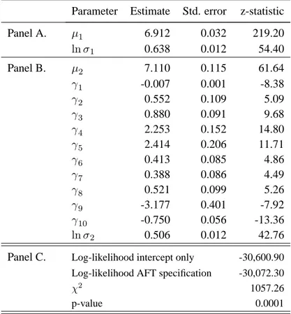
This section presents the estimation results for our specification of time to efficiency, using the maximum likelihood approach described in section 2.3.4. The estimation is first performed using an intercept-only specification (without covariates) in order to infer the general pattern of our sample times based on the shape and scale estimates of the underlying Weibull distribution. We then turn to the estimation of our accelerated-failure time specification using the whole set of covariates that we previously defined. The estimated parameters for the two specifications along with standard errors and z-statistics are reported in Table 215
[Table 2 about here.]
We first restrict our attention to the general pattern of survival times we obtain through the estimates from the intercept-only model. We then analyze the estimates from the AFT specification and detail the effect of our explanatory variables.
Using (16) to transform the ˆµ1 and ˆσ1 estimates back onto the original time scale gives the
corresponding ˆα = 0.528 and ˆλ = 0.026 values for the underlying Weibull distribution. From the former, it appears that the sample TTEs exhibit a decreasing hazard rate, so that the prob-ability of an arbitrage opportunity disappearing in the next instant is higher shortly after it has been detected than after a long time period has elapsed. Probably, this (unconditional) pattern simply reflects differences across arbitrage opportunities according to the arbitrage profit they give rise to. Large profit opportunities may trigger immediate reaction from market participants thus resulting in a very short time to efficiency. On the contrary, small profit opportunities may be kind of neglected by traders as the total cost, combined with the associated risk and the difficulties they face when building the arbitrage portfolio, could result in a net loss.
14Notice that the Parkinson estimator requires regularly-spaced price series, which is the case here since the
CAC 40 index value is disseminated every 30 seconds.
15An intercept-only specification is necessary here to estimate the shape and scale parameters of the underlying
distribution as the intercept in the AFT specification is contaminated by the effect of dummy variables on maturity and moneyness class.
Estimates associated with our explanatory variables somehow confirm this story while bring-ing additional interestbring-ing information. The first thbring-ing to note is that the variables we use have overall explanatory power as the likelihood ratio test leads to a 1057.26 value for the chi-square with an associated 0.0001 p-value. Second, variables are all significantly different from zero at conventional levels when considered individually. We know analyze them in turn.
The coefficient on variable ActivOpt is negative with z-statistic −8.38, indicating that the most active the options market, the shorter the time to efficiency. On the contrary, the coefficient on variable RatioOpt is significantly positive, which implies that the larger the trades imbalance between call and put options, the longer the time to efficiency. This is not surprising since difficulties to match, say a call option, with the corresponding put option will make things harder and longer for a given trader when she has to build the appropriate arbitrage portfolio. Overall, the results from the ActivOpt and RatioOpt variables suggest that the liquidity on the options market is a significant determinant for time to efficiency.
The coefficients on variables Mat2–Mat4, and MoneyClass2–MoneyClass4 are all positive and significantly different from zero. The positive coefficients we get on Mat2 to Mat4 are con-sistent with the liquidity argument since the nearest contracts are the most actively traded ones. By contrast, the coefficients on the moneyness dummy variables are more intriguing. In line with the liquidity argument, we would expect a negative coefficient on variables MoneyClass2 and MoneyClass3 since near at-the-money options are usually more frequently traded than other options. Remember however that from our definition of moneyness classes, options belonging to class 1 include both deeply out-of-the-money call options and deeply in-the-money put op-tions, with the latter being rather actively traded by investors who seek to protect their portfolio against downward market movements. In this view, the positive coefficients associated to the moneyness classes 2 to 4 reflect a lower liquidity for these options compared with the liquidity of the deeply out-of-the-money put options market.
We now turn to the determinants in connection with the underlying index. We find evidence of a significant negative relationship between volatility and time to efficiency. This is an inter-esting result since the direction of the effect was rather unpredictable. On the one hand, in line with Kamara and Miller (1995), volatility makes arbitrage riskier since it increases the prob-ability for a trader to face adverse price changes by the time she is in the process of building the arbitrage portfolio. This should result in a longer time to efficiency. On the other hand, a mechanistic effect is at work by which a greater volatility increases the probability for the index value to be consistent with the put-call parity relationship in the next instant. Notice that this situation should occur more frequently in presence of ‘small’ arbitrage opportunities, but overall the mechanistic effect appears to be the dominant one in our sample.
Finally the negative coefficient on the ETF variable indicates that the introduction of the CAC 40 ETF by January 21, 2001 resulted in a shorter time to efficiency, and thus in an im-proved efficiency. This result may be compared with the findings of Ackert and Tian (1998, 2001) who find that the introduction of ETFs did not contributed to reduce ex post profits, nei-ther on the Canadian market nor on the US market. However, it is consistent with the evidence in Kurov and Lasser (2002) who document a negative relationship between the existence of the QQQ ETF on Nasdaq and the size of arbitrage profits on the corresponding futures contracts. However, our results provide a somewhat different information: by making trades on the under-lying index easier, the ETF allows market participants to react in a shorter time interval once an arbitrage opportunity has been detected.
4.3
Checking model adequacy
To assess the appropriateness of our econometric specification, we performed a graphical (haz-ard plot) test of goodness-of-fit in the spirit of Lo, MacKinlay and Zhang (2002). Graphical tests are informal tests as “they serve as a means of rejecting clearly inappropriate models, not to ‘prove’ that a particular model is correct” (Klein and Moschberger, 2003). The underlying principle is to check whether the distribution of times-to-event, conditional on a set of covari-ates, follows the postulated distribution. In our case, this amounts to testing whether TTEs, conditional on our explanatory variables, follow a Weibull distribution.
To do so, we proceed in the following way. We first compute the set of standardized residuals {ˆui} as: ˆ ui = ln Ti − ˆµ2− γ0Zi ˆ σ2 (22)
If the Weibull specification holds, then, according to (19), the {ˆui} should behave like a
cen-sored sample from a standard extreme value distribution. To check this point, we compute the Kaplan-Meier16 estimator ˆS({ˆu
i}) of the survival curve from the {ˆui}. Taking minus the log,
this yields the integrated hazard ˆΛ({ˆui}). Using (20), the expression for the integrated hazard
of a standard extreme value distribution is found to be:
ΛU(u) = exp(u) (23)
Hence, if our Weibull specification holds, a plot of {ˆui} against {ln[ˆΛ(ˆui)]} should be a straight
16The Kaplan-Meier estimator is a non-parametric technique which allows to compute the empirical survival
function from a sample including censored observations. Interested readers may refer to the original article, Kaplan-Meier (1958), or to Lo, MacKinlay and Zhang (2002).
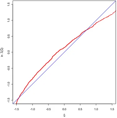
line with intercept 0 and slope 1. The result from the plot is reported in Figure 3. Although we observe some departures from the expected straight line, these are sufficiently small to consider that our model reasonably fit the data17.
[Figure 3 about here.]
4.4
Implications for time to efficiency
Having tested the appropriateness of our specification and with parameter estimates in hands, we are now interested in computing the implications of our model for the survival of arbitrage opportunities through a sensitivity analysis. In order to study to which extent initial market conditions (Zi) impact the time to efficiency, we compute the corresponding survival function
SW[t exp(−γ0Zi)], using the Weibull specification (see eq. 12) for the baseline survival function
SW. The analysis is performed for each of the determinants we identified by allowing the
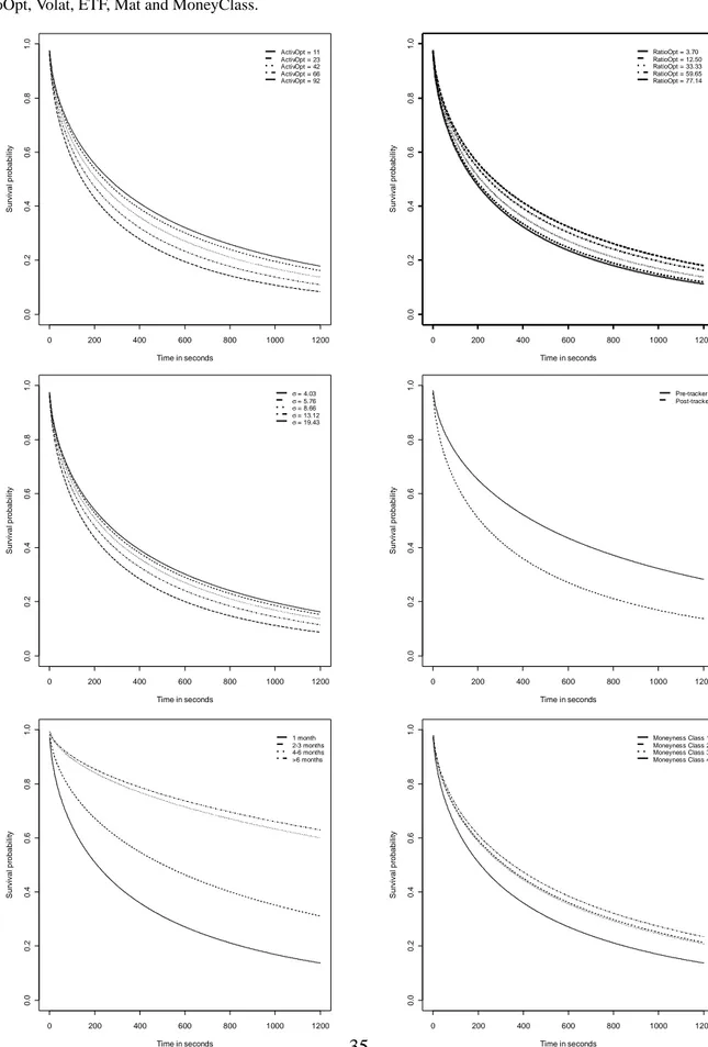
explanatory variable of interest to take its 10%, 25%, 50%, 75% and 90% percentile values while all other explanatory variables are held fixed at their sample median value18. The results
are reported in figure 4.
[Figure 4 about here.]
Figure 4 shows, as expected, that the higher the volatility, the higher is the probability the arbitrage opportunity has disappeared over any given time interval. However, the differences in estimated survival curves are not so important. If we consider for example the situation that prevails 20 minutes after an arbitrage opportunity has been detected, the probability for the market to remain in a state of profitable arbitrage is 8.73% for the highest 10% volatilities versus 16.27% for the lowest 10%. This conclusion remains valid for the ActivOpt and the RatioOpt variables. If we refer to the former, it appears that the estimated survival probability after a 20-minute interval is 8.33% for the highest 10% ActivOpt values versus 17.81% for the lowest 10%. Regarding the RatioOpt variable, the difference is only 6.81% between the top and the bottom decile (18.00% versus 11.20% respectively).
17We also performed hazard plot tests using other specifications for the underlying distribution of times, namely
exponential, log-logistic and log-normal. The hazard plots we obtained clearly reject the exponential specification, whereas the other two distribution yield clearly inferior, though acceptable fit compared with the Weibull specifi-cation. We also tried to fit the data using a generalized gamma specification, but were unable to get converging result when performing the likelihood maximization. All results are available upon request.
18When fixed, dummy variables are assigned the following values: ETF = 1, Mat2 = 0, Mat3 = 0, Mat4 = 0,
MoneyClass2 = 0, MoneyClass3 = 0, MoneyClass4 = 0, so that computations are performed in presence of the
Variables referring to maturity, moneyness and the existence of the ETF yield more distinct patterns across the different values we use for the underlying determinant. The most dramatic differences are observed with respect to the maturity class. For the longest maturities, the estimated probability an arbitrage opportunity has survived after 20 minutes is 62.98%, with a corresponding 13.76% probability for the shortest maturities. It takes only 3:29 minutes for half of the opportunities to disappear for the shortest maturities whereas 85.12% of them are still alive at the same time if the underlying options is to expire after six months. The same conclusion apply to the dummy variables associated with the moneyness classes. 23.49% of the moneyness class 4 arbitrage opportunities are still alive after 20 minutes, but this figure drops to 13.76% for the moneyness class 1 options. Moreover, there are only slight differences across options belonging to the moneyness classes 2 to 4. Overall, these results stress the importance of the intrinsic liquidity and options characteristics for the profitability of arbitrage-based strategies and the efficiency of the options market. Also, an implication of these results is that arbitrageurs tend to concentrate their actions on the options series which, by their very nature, are likely to be the most active.
We finally turn to the ETF variable. As stated before, the existence of an ETF on the under-lying CAC 40 index resulted in a shorter time to efficiency. More precisely, results associated with the estimated survival curves show that we get an estimated 28.32% probability for an arbitrage opportunity to be still alive by 20 minutes prior the ETF was introduced, a figure that drops to 13.76% after the introduction.
4.5
Additional analysis
4.5.1 Nearby maturity
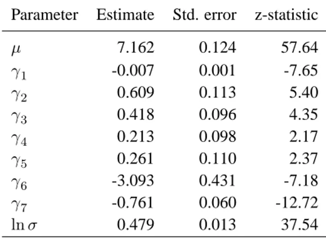
So far our estimates have been computed over the whole sample of arbitrage opportunities we identified. As stated before however, most of the arbitrageurs’ activity tends to concentrate on the nearby options contracts. As a consequence, it would be interesting to study to which extent our results are affected when computations are performed on this particular subset of 3,380 matching pairs.
Parameter estimates reported in Table 3 bring several interesting results. First of all, the coefficient on the activity of the options market is smaller than in the full-sample case. This is a fairly intuitive result since we now focus on the most liquid options so that the possibility to eas-ily trade a given option is somehow guaranteed. The same argument applies to the moneyClass variables which exhibit smaller coefficients (with the exception of the moneyClass2 variable). On the contrary, the RatioOpt variable gains in importance. We explain it as follows: since the
1-month contracts are the most liquid, arbitrageurs are less concerned with the possibility to trade a given option whereas they focus on the possibility to build the arbitrage portfolio, so that differential liquidity between call and put options now becomes a major determinant of an arbitrage opportunity persisting over time.
[Table 3 about here.]
Variables related to the underlying asset also provide valuable information. The coefficient on the volatility is now -3.093 versus -3.177 for the full sample analysis, so that the TTE appears to be less sensitive to the index volatility for the nearby contracts compared with longer matu-rities. This result is consistent with the mechanistic argument we developed in section 4.2. As the nearby contracts are the ones for which the arbitrageurs’ activity is most pronounced, prices returning to compatible levels in this case are more likely to result from efficiency-creating actions by arbitrageurs rather than random fluctuations from the underlying index. Finally the coefficient on the ETF variable exhibits no significant change.
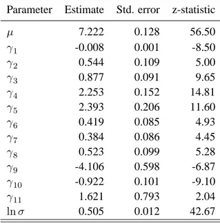
4.5.2 Interaction between volatility and ETF
A final question we want to address is whether the existence of an ETF tracking the underlying index has an incidence on the way the underlying volatility impacts the time to efficiency. Mo-tivation for this question arises from the potential ambiguous role of volatility we mentioned above. On the one hand, previous estimates yield to the conclusion that there exists a nega-tive relationship between volatility and time to efficiency, a result we attributed to the so-called mechanistic effect of volatility on prices. On the other hand we suggested that higher volatil-ity might result in higher risk for arbitrageurs due to adverse price movements, thus leading to longer time to efficiency.
To explore more thoroughly this relationship, we proceed to a new estimation of our AFT specification using a model that incorporates an additional Interact term which we define as:
Interact ≡ V olat × ET F
Parameter estimates for the whole 4,271 sample matchings are reported in Table 4.
[Table 4 about here.]
The results help reconciling the conflicting views we previously mentioned. First of all, the coefficient associated with volatility becomes larger in magnitude suggesting that volatility per
se actually tends to reduce the time to efficiency through the mechanistic effect. The same result is observed for the existence of the ETF, so that the possibility to trade the underlying index through an ETF on a continuous market makes arbitrage easier. Finally, the coefficient on the Interact variable is positive but only weekly significant with z-statistic 2.04 and an associated p-value of 0.041. Overall, these results suggest that the risk of adverse movements is more pronounced in illiquid market for the underlying asset as the joint incidence of ETF and Volat, after removing the effect the ETF variable, is negligible.
5
Conclusion
Using the concept of TTE, this article sheds light on the determinants which govern the speed at which an index options market converges to a state of efficiency after an arbitrage opportunity has been detected. To achieve this goal, we make use of a statistical technique called survival analysis. We find that the Weibull distribution along with an accelerated failure time specifica-tion provides a sensible fit to the data and that the TTE is quite sensitive to several explanatory variables. The activity on the options markets as well as the possibility to easily match a given call option with the corresponding put option significantly influence the TTE. We also docu-ment that differences in options characteristics (namely moneyness and distance to maturity) lead to important changes in the probability for an arbitrage opportunity to survive over a given time-interval. Regarding the underlying asset, we find that survival times are shorter when the index volatility is high. Finally, the introduction of an ETF replicating the underlying index re-sults in shorter TTEs, even after controlling for market conditions, thus underlying the positive effect this new instrument has on index derivatives markets efficiency.
References
ACKERT, L. F.,ANDY. S. TIAN(1998): “The Introduction of Toronto Index Participation Units
and Arbitrage Opportunities in the Toronto 35 Index Option Market,” Journal of Derivatives, 5(4), 44–53.
(2001): “Efficiency in Index Options Markets and Trading in Stock Baskets,” Journal of Banking and Finance, 25(9), 1607–1634.
BHARADWAJ, A., ANDJ. B. WIGGINS (2001): “Box Spread and Put-Call Parity Tests for the
S&P 500 Index LEAPS Market,” Journal of Derivatives, 8(4), 62–71.
BILLINGSLEY, R. S., AND D. M. CHANCE(1985): “Options Markets Efficiency and the Box
Spread Strategy,” Financial Review, 20(4), 287–301.
BISIÈRE, C., AND T. KAMIONKA(2000): “Timing of Orders, Orders Aggressiveness and the
Order Book at the Paris Bourse,” Annales d’Économie et de Statistiques, (60), 43–72.
CAPELLE-BLANCARD, G., AND M. CHAUDHURY (2001): “Efficiency Tests of the French
Index (CAC 40) Options Market,” Working paper, McGill University.
CASSESE, G., AND M. GUIDOLIN (2001): “Pricing and Informational Efficiency of the
MIB30 Index Options Market,” Working paper, University of Southern Switzerland, http://www.lu.unisi.ch/istfin/papers/gianluca.pdf.
CAVALLO, L., AND P. MAMMOLA(2000): “Empirical Tests of Efficiency of the Italian Index
Options Market,” Journal of Empirical Finance, 7, 173–193.
CHANCE, D. M. (1987): “Parity Tests of Index Options,” Advances in Futures and Options
Research, 2, 47–64.
CHESNEY, M., R. GIBSON,AND H. LOUBERGÉ(1995): “Arbitrage Trading and Index Option
Pricing at SOFFEX: An Empirical Study Using Daily and Intradaily Data,” Finanzmarkt und Portfolio Management, 9(1), 35–60.
CHORDIA, T., R. ROLL, AND A. SUBRAHMANYAM (2004): “Evidence on the speed of
con-vergence to market efficiency,” Forthcoming in the Journal of Financial Economics.
DEVILLE, L. (2004): “Time to Efficiency on Options Markets and the Introduction of ETFs:
Evidence from the French CAC 40 Index,” Working Paper, Paris Dauphine University.
EVNINE, J.,ANDA. RUDD(1985): “Index Options: The Early Evidence,” Journal of Finance,
40(3), 743–756.
FINUCANE, T. J. (1991): “Put-Call Parity and Expected Returns,” Journal of Financial and
GALAI, D. (1977): “Tests of Market Efficiency of the Chicago Board Options Exchange,”
Journal of Business, 50(2), 167–197.
GOULD, J., ANDD. GALAI(1974): “Transaction Costs and the Relationship between Put and Call Prices,” Journal of Financial Economics, 1, 105–129.
GREENE, W. H. (2002): Econometric Analysis. Prentice Hall, Englewood Cliffs, NJ, 4 edn.
KAMARA, A., AND T. W. MILLER (1995): “Daily and Intradaily Tests of Put-Call Parity,”
Journal of Financial and Quantitative Analysis, 30(4), 519–539.
KAPLAN, E. L., AND P. MEIER(1958): “Nonparametric Estimation from Incomplete
Obser-vations,” Journal of the American Statistical Association, 53, 457–481.
KIEFER, N. (1988): “Economic Duration Data and Hazard Functions,” Journal of Economic
Litterature, 26, 646–679.
KLEIN, J., ANDM. MOESCHBERGER (2003): Survival analysis: techniques for censored and
truncated data, Statistics for biology and health. Springer, 2nd edn.
KLEMKOSKY, R. C., AND B. G. RESNICK (1979): “Put-Call Parity and Market Efficiency,”
Journal of Finance, 34(5), 1141–1155.
(1980): “An Ex-Ante Analysis of Put-Call Parity,” Journal of Financial Economics, 8, 363–378.
KUROV, A. A., AND D. J. LASSER (2002): “The Effect of the Introduction of Cubes on the
Nasdaq-100 Index Spot-Futures Pricing Relationship,” Journal of Futures Markets, 22(3), 197–218.
LO, A., C. MACKINLAY, ANDJ. ZHANG (2002): “Econometric models of limit-order
execu-tions,” Journal of Financial Economics, 65, 31–71.
MERTON, R. C. (1973): “The Relationship between Put and Call Prices: Comment,” Journal
of Finance, 28(1), 183–184.
MITTNIK, S., AND S. RIEKEN (2000): “Put-Call Parity and the Informational Efficiency of
the German DAX-Index Options Market,” International Review of Financial Analysis, 9, 259–279.
PARKINSON, M. (1980): “The Extreme Value Method for Estimating the Variance of the Rate
of Return,” Journal of Business, 53, 61–65.
PUTTONEN, V. (1993): “Boundary Conditions for Index Options: Evidence from the Finnish
Market,” Journal of Futures Markets, 13(5), 545–562.
STOLL, H. R. (1969): “The Relationship between Put and Call Option Prices,” Journal of
WAGNER, D., D. M. ELLIS, AND D. A. DUBOFSKY (1996): “The Factors Behind Put-Call
Table 1: Time to efficiency statistics
This Table reports descriptive statistics of our sample of put-call parity matching pairs (upper part of the Table) by time to maturity, and of the calculated times to censoring (Sample A) and times to efficiency (Sample B) both for the whole period and for the periods preceding (August 1, 2000 to January 21, 2001) and following (January 22,
2001 to July 31, 2001) the introduction of the CAC 40 Master Unit ETF. Asterisks∗∗∗denotes the rejection of the
equality between pre- and post-ETF central values at the 1% level in unilateral tests.
Full Before After
Sample Introduction Introduction
Observations 4,279 1,733 2,546
by time to maturity
less than 1 month 3,380 1,420 1,960
2-3 months 567 208 359
4-6 months 209 48 161
7-12 months 115 53 62
Sample A: no reversion to efficient prices before the market close
number 432 178 254
proportion 10.10 10.27 9.98
Time to censoring (minutes)
mean 106.27 147.17 77.06
median 31.83 68.77 13.88
Sample B: reversion to efficient prices before the market close
number 3,847 1,555 2,292
proportion 89.90 89.73 90.02
Time to efficiency (minutes)
mean 19.22 27.00 13.93
t-test 7.91∗∗∗
median 3.60 4.90 3.32
Table 2: Parameter estimates
This Table reports the maximum likelihood parameter estimation for the 4,271 sample matchings. Results in Panel A are for the intercept-only specification
ln T = µ1+ σ1u1
Results in Panel B are for the accelerated-failure-time specification
ln T = µ2+ γ1ActivOpt + γ2RatioOpt + γ3Mat2 + γ4Mat3 + γ5Mat4 +γ6MoneyClass2 + γ7MoneyClass3 + γ8MoneyClass4
+γ9Volat + γ10ETF + σ2u2
where u1and u2are error terms which follow a standard extreme value distribution.
Parameter Estimate Std. error z-statistic
Panel A. µ1 6.912 0.032 219.20 ln σ1 0.638 0.012 54.40 Panel B. µ2 7.110 0.115 61.64 γ1 -0.007 0.001 -8.38 γ2 0.552 0.109 5.09 γ3 0.880 0.091 9.68 γ4 2.253 0.152 14.80 γ5 2.414 0.206 11.71 γ6 0.413 0.085 4.86 γ7 0.388 0.086 4.49 γ8 0.521 0.099 5.26 γ9 -3.177 0.401 -7.92 γ10 -0.750 0.056 -13.36 ln σ2 0.506 0.012 42.76
Panel C. Log-likelihood intercept only -30,600.90
Log-likelihood AFT specification -30,072.30
χ2 1057.26
Table 3: Parameter estimates for the nearby contracts
This Table reports the maximum likelihood parameter estimates for the nearby contracts 3,380 sample matchings using the accelerated-failure-time specification
ln T = µ + γ1ActivOpt + γ2RatioOpt
+γ3MoneyClass2 + γ4MoneyClass3 + γ5MoneyClass4 +γ6Volat + γ7ETF + σu
where u is an error term which follows a standard extreme value distribution.
Parameter Estimate Std. error z-statistic
µ 7.162 0.124 57.64 γ1 -0.007 0.001 -7.65 γ2 0.609 0.113 5.40 γ3 0.418 0.096 4.35 γ4 0.213 0.098 2.17 γ5 0.261 0.110 2.37 γ6 -3.093 0.431 -7.18 γ7 -0.761 0.060 -12.72 ln σ 0.479 0.013 37.54
Table 4: Interaction between volatility and ETF
This Table reports the maximum likelihood parameter estimates for the 4,271 sample matchings using the accelerated-failure-time specification
ln T = µ + γ1ActivOpt + γ2RatioOpt + γ3Mat2 + γ4Mat3 + γ5Mat4 +γ6MoneyClass2 + γ7MoneyClass3 + γ8MoneyClass4
+γ9Volat + γ10ETF + γ11Interact + σu
where u is an error term which follows a standard extreme value distribution.
Parameter Estimate Std. error z-statistic
µ 7.222 0.128 56.50 γ1 -0.008 0.001 -8.50 γ2 0.544 0.109 5.00 γ3 0.877 0.091 9.65 γ4 2.253 0.152 14.81 γ5 2.393 0.206 11.60 γ6 0.419 0.085 4.93 γ7 0.384 0.086 4.45 γ8 0.523 0.099 5.28 γ9 -4.106 0.598 -6.87 γ10 -0.922 0.101 -9.10 γ11 1.621 0.793 2.04 ln σ 0.505 0.012 42.67
Figure 1: Intradaily distributions of call transactions, put transactions and put-call parity syn-chronous pairings
Figure 2: Empirical densities of times to censoring (left figure, 432 observations) and times to efficiency (right figure, 3,847 observations)
Time to efficiency Time in seconds D e n s it y 0 5000 10000 15000 20000 0.0000 0.0005 0.0010 Time to censoring Time in seconds D e n s it y 0 10000 20000 30000 0.00000 0.00005 0.00010 0.00015
Figure 3: Test of Goodness-of-fit
The graph plots the log of the integrated hazard of the standardized residuals based on the Kaplan-Meier estimator of their empirical survival curve (ln[ ˆΛ(ˆu)]), against the standardized residuals (ˆu). Standard-ized residuals are computed using (22). Under appropriate specification for the model, the graph should coincide with the plotted straight line.
-1.5 -1.0 -0.5 0.0 0.5 1.0 1.5 -1 .5 -1 .0 -0 .5 0 .0 0 .5 1 .0 1 .5 u ^ ln Λ ^( u^ )
Figure 4: Sensitivity analysis
Those figures plot the estimated survival functions for different levels of the explanatory variables ActivOpt, Ra-tioOpt, Volat, ETF, Mat and MoneyClass.
0 200 400 600 800 1000 1200 0 .0 0 .2 0 .4 0 .6 0 .8 1 .0 Time in seconds S u rv iv a l p ro b a b il it y ActivOpt = 11 ActivOpt = 23 ActivOpt = 42 ActivOpt = 66 ActivOpt = 92 0 200 400 600 800 1000 1200 0 .0 0 .2 0 .4 0 .6 0 .8 1 .0 Time in seconds S u rv iv a l p ro b a b il it y RatioOpt = 3.70 RatioOpt = 12.50 RatioOpt = 33.33 RatioOpt = 59.65 RatioOpt = 77.14 0 200 400 600 800 1000 1200 0 .0 0 .2 0 .4 0 .6 0 .8 1 .0 Time in seconds S u rv iv a l p ro b a b il it y σ = 4.03 σ = 5.76 σ = 8.66 σ = 13.12 σ = 19.43 0 200 400 600 800 1000 1200 0 .0 0 .2 0 .4 0 .6 0 .8 1 .0 Time in seconds S u rv iv a l p ro b a b il it y Pre-tracker Post-tracker 0 .2 0 .4 0 .6 0 .8 1 .0 S u rv iv a l p ro b a b il it y 1 month 2-3 months 4-6 months >6 months 0 .2 0 .4 0 .6 0 .8 1 .0 S u rv iv a l p ro b a b il it y Moneyness Class 1 Moneyness Class 2 Moneyness Class 3 Moneyness Class 4