Symmetry and symmetry breaking:
rigidity and flows in elliptic PDEs
Jean Dolbeault, Maria J. Esteban, and Michael Loss
Abstract
The issue of symmetry and symmetry breaking is fundamental in all areas of science. Symmetry is often assimilated to order and beauty while symmetry breaking is the source of many interesting phenomena such as phase transi-tions, instabilities, segregation, self-organization, etc. In this contribution we review a series of sharp results of symmetry of nonnegative solutions of non-linear elliptic differential equation associated with minimization problems on Euclidean spaces or manifolds. Nonnegative solutions of those equations are unique, a property that can also be interpreted as a rigidity result. The method relies on linear and nonlinear flows which reveal deep and robust properties of a large class of variational problems. Local results on linear instability leading to symmetry breaking and the bifurcation of non-symmetric branches of solu-tions are reinterpreted in a larger, global, variational picture in which our flows characterize directions of descent.
1. INTRODUCTION
Symmetries are fundamental properties of the laws of Physics. They impose
con-straints on modeling phenomena and, at a more basic level, they serve as criteria of classification. Inspired by his work in crystallography, Pierre Curie made an early attempt (in 1894) to investigate the consequences of symmetries. Since then, sym-metry has been an important preoccupation for many scientists.
More intriguing than symmetry is the phenomenon of symmetry breaking, which asserts that the state of a system may have less symmetries than the underlying physical laws. Among various considerations on the causes of the symmetries and what these symmetries mean in physics, P. Curie wrote in [12] that
C’est la dissymétrie qui crée le phénomène.
In mathematical terms, “dissymétrie” shifts the attention to solutions which may have less symmetries than the problem they solve. Symmetry breaking, especially Keywords: Symmetry; symmetry breaking; interpolation inequalities;
Caffarelli-Kohn-Niren-berg inequalities; optimal constants; rigidity results; fast diffusion equation; carré du champ; bifurcation; instability. – MSC (2010): 35J20; 49K30, 53C21.
Acknowledgements: Partially supported by the projects Kibord and EFI (J.D.) of the French
spontaneous symmetry breaking, has been an incredibly fruitful concept over the last century. It appears in mechanics (buckling instabilities), in particle physics, in the description of phase transitions or complex dynamics, etc. One of the ba-sic mechanisms is the bifurcation phenomenon in nonlinear systems, which has to do with the stability analysis of symmetric states.
Symmetry has attracted the attention of mathematicians for diverse reasons which range from assertions like “symmetry is beautiful” to practical motivations: symme-try simplifies the search of solutions and makes their computation more tractable from a numerical point of view by reducing the number of degrees of freedom.
Entropy methods have a long history in various fields of Science and in particular
of Mathematics. The notion of entropy that we shall consider here is inspired by re-sults in the theory of nonlinear PDEs and especially nonlinear diffusion equations. It borrows tools from Kinetic Theory and from Information Theory. Other major sources of inspiration are the carré du champ method used in the study of Semi-groups and Markov processes as well as the rigidity (uniqueness) techniques in the Theory of Nonlinear Elliptic Equations. In addition to the application to symmetry issues, one of our contributions was to rephrase these two approaches in a common framework of parabolic equations and to emphasize the role of the nonlinear diffu-sions in the search for optimal ranges and optimal constants in related interpolation inequalities.
It is definitely out of reach to give even a partial account of all mathematical issues of symmetry and symmetry breaking in this paper, so we shall focus on PDEs with two main examples: the first one is the equation
−div¡|x|−β∇w¢ = |x|−γ¡w2p−1− wp¢
in Rd\ {0},
which has an interesting feature: there is a competition between nonlinearities and weights. The solutions can be interpreted as critical points of an energy functional. Without weights, solutions are radially symmetric (up to translations). With weights and in some regime of the parameters β, γ and p, non-radial solutions are energet-ically more favorable. Since we are interested in energy minimizers, as a particular sub-problem, understanding who wins in the competition is a central question.
Alternatively, we shall consider the equation −∆ϕ + Λϕ = ϕp−1 on M ,
where M is a sphere, a compact manifold or a cylinder. In that case, the geometric properties of the manifold replace the weight and compete with the scale induced by the parameter Λ. If there is enough space, in a precise sense that can be measured, then solutions with less symmetry may have a lower energy.
These two equations, although very simple because the nonlinearities (and also the weights in the case of the first equation) obey power laws, are not purely aca-demic. For one, the solutions (and the associated functional inequalities) are of direct interest for instance in some models of fluid mechanics. More important is the fact that power laws appear in many problems when scalings or blow-up meth-ods are used to extract an asymptotic behavior. Hence, we expect that our model equations lie at the core of many nonlinear or weighted problems. Finally, models
involving power laws have the advantage that they can be treated by using
nonlin-ear flows and entropy methods. Indeed we are able to give sharp results of rigidity
for the equation, and symmetry results for the optimal functions associated with related interpolation inequalities.
Because of the confluence of various branches of analysis such as non-linear dif-fusion and the calculus of variations, and the fundamental nature of the above equa-tions, we believe that it is worth studying them in great detail, with sharp stability results and sharp constants in the functional inequalities. Note that this amounts to establishing the exact range of the parameters for which extremal functions are sym-metric. Variational issues of the symmetry and symmetry breaking will be detailed below.
Let us fix some notations and conventions. Throughout this paper, we shall use the notation 2∗:= 2d
d −2if d ≥ 3, and 2∗:= ∞ if d = 1 or 2. We shall say that a function is an extremal function for an optimal functional inequality if equality holds in the inequality. To simplify notations, parameters will be omitted whenever they are not essential for the understanding of the strategy of proof. This paper is a review of various results which were published in several papers (references will appear in the text) and are collected together for the first time. The reader is invited to pay attention that some notations have been redefined compared to the original papers.
2. INTERPOLATION INEQUALITIES AND FLOWS ON COMPACT MANIFOLDS 2.1. Interpolation inequalities on Sd. Let us consider the inequality
k∇uk2L2(Sd)+ d p − 2kuk 2 L2(Sd)≥ d p − 2kuk 2 Lp(Sd) ∀u ∈ H 1(Sd,dµ) (1)
where dµ is the uniform probability measure induced by the Lebesgue measure on Sd⊂ Rd +1. Here the exponent p is such that 1 ≤ p < 2 or 2 < p < 2∗, or p = 2∗if
d ≥ 3. The case p = 2∗corresponds to the usual Sobolev inequality on Sdor, using the stereographic projection, to the Sobolev inequality in Rd. In the limit case as
p → 2, we recover the logarithmic Sobolev inequality
k∇uk2L2(Sd)≥ d 2 ˆ Sd|u| 2log à |u|2 kuk2L2(Sd) ! d µ ∀u ∈ H1(Sd,dµ) \ {0}. (2) In (1) and (2), equality is achieved by any constant non-zero function. The value of the optimal constants, d/(p − 2) and d/2 is obtained by linearization: if ϕ is an eigenfunction associated with the first positive eigenvalue of the Laplace-Beltrami operator on Sd, the infimum of
(p − 2)k∇uk2L2(Sd) kuk2Lp(Sd)− kuk 2 L2(Sd) and 2k∇uk 2 L2(Sd) ´ Sd|u|2log ³ |u|2 kuk2L2(Sd ) ´ d µ ,
Inequality (1) has been established in [8] by rigidity methods, in [6] by tech-niques of harmonic analysis, and using the carré du champ method in [7,5,14], for any p > 2. The case p = 2 was studied in [39]. In [1,2,3], D. Bakry and M. Emery proved the inequalities under the restriction
2 < p ≤ 2#:=2d 2+ 1 (d − 1)2.
Their method relies on a linear heat flow method which is presented below, as well as a nonlinear flow which allow us to get rid of this restriction.
2.2. Flows and carré du champ methods on Sd. We start by the linear heat flow method of [3]. For any function ρ > 0 we define a generalized entropy functional Ep and a generalized Fisher information functional Ipby
Ep[ρ] := 1 p − 2 " µˆ Sdρ d µ ¶2 p − ˆ Sdρ 2 pd µ # and E2[ρ] :=1 2 ˆ Sdρ log à ρ kρkL1(Sd) ! d µ if p 6= 2 or p = 2, respectively, and Ip[ρ] := ˆ Sd|∇ρ 1 p|2d µ .
With this notation, (1) and (2) amount to Ip[ρ] ≥ d Ep[ρ] as can be checked using
ρ = |u|p. Let us consider the heat flow
∂ρ
∂t = ∆ρ (3)
where ∆ denotes the Laplace-Beltrami operator on Sd, and compute
d
d tEp[ρ] = −2Ip[ρ] and d
d tIp[ρ] ≤ −2d Ip[ρ]
where the differential inequality holds if p ≤ 2#. Under this condition, we obtain that
d d t ³ Ip[ρ] − d Ep[ρ] ´ ≤ 0.
On the other hand, ρ(t,·) converges as t → ∞ to a constant, namely´
Sdρ d µ since
d µ is a probability measure and´Sdρ d µ is conserved by (3). As a consequence, limt →∞¡Ip[ρ] − d Ep[ρ]¢ = 0, which proves that Ip[ρ(t,·)] −d Ep[ρ(t,·)] is nonneg-ative for any t ≥ 0 and completes the proof. See [3] for details. One may wonder whether the monotonicity property is also true for some p > 2#. The following result contains a negative answer to this question.
Proposition 1. [27] For any p ∈ (2#,2∗) or p = 2∗if d ≥ 3, there exists a function ρ0
such that, if ρ is a solution of (3) with initial datum ρ0, then
d d t ³ Ip[ρ] − d Ep[ρ] ´ |t=0> 0.
The function ρ0is explicitly constructed in [27].
To overcome the limitation p ≤ 2#, one can consider a nonlinear diffusion of fast diffusion or porous medium type
∂ρ ∂t = ∆ρ
m. (4)
With this flow, we no longer have d
d tEp[ρ] = −Ip[ρ] but we can still prove that
d d t
³
Ip[ρ] − d Ep[ρ]´≤ 0,
for any p ∈ [1,2∗]. Proofs of the latter have been given in [14,24]. We also refer to [21,22] for results which are more specific to the case of the sphere, and further references therein. Except for p = 1 and p = 2∗with d ≥ 3, there is some flexibility in the choice of m, which can be used to build deficit functionals and improved inequalities: see [14,22]. Notice that ρ0in Proposition1is a function related with the nonlinear diffusion equation (4).
The case of Sd highlights the limitations of linear flows and shows the flexibil-ity and strength of nonlinear flows. At least for p < 2∗, the optimal constant in (1) and (2) is established by proving that the minimum of Ip[ρ] − d Ep[ρ] is 0. Earlier results in [8,5,6] can be reinterpreted as a purely elliptic method, which goes as fol-lows. A positive minimizer actually exists by standard compactness arguments and any solution ρ satisfies an Euler-Lagrange equation. By testing the equation with ∆ρm, we observe that the solution is a constant and, as a consequence, that ρ ≡ 1 because of the normalization. We will rely on a similar observation in the next two sections and refer to this method as the elliptic method.
The method applies not only to minimizers, but also to any positive solution of the Euler-Lagrange equations. What we prove is a uniqueness result. Since constant functions are solutions, this proves that there are no non-constant solutions. This is why it is called a rigidity result.
Compared to [8,5,6], our approach provides a unified framework for p > 2 and
p < 2 (which is not covered in the above mentioned results). However, the main
advantage of the method is that it explains why a local result (the best constant is given by the linearization around the constant functions) is actually global: Ip[ρ] −
d Ep[ρ] is strictly monotone decreasing under the action of the flow, unless the so-lution has reached the unique, trivial stationary state.
2.3. Inequalities on compact manifolds. The nonlinear diffusion flow method ap-plies not only to spheres, but also to general compact manifolds. Without entering in the details, let us state a result of [24]. Earlier important references are: [35,8,38,14], among many other contributions which are listed in [24].
Let us assume that (M , g ) is a smooth compact connected Riemannian mani-fold of dimension d ≥ 1, without boundary. We denote by dvgthe volume element, by ∆ the Laplace-Beltrami operator on M , by Ric the Ricci tensor and assume for
simplicity that volg(M ) = 1. Let λ1be the lowest positive eigenvalue of −∆ and λ⋆:= inf u∈H2(M ) ˆ M h (1 − θ)(∆u)2+d −1θ d Ric(∇u,∇u)id vg ´ M|∇u|2d vg , θ = (d − 1) 2(p − 1) d (d + 2) + p − 1. Theorem 2. With the above notations, if 0 < λ < λ⋆, then for any p ∈ (1,2) ∪ (2,2∗),
the equation
−∆v + λ
p − 2¡v − v
p−1¢ = 0
has a unique positive solution in C2(M ), which is constant and equal to 1.
It has been shown in [24] that nonlinear diffusion flows provide a unified frame-work for elliptic rigidity and carré du champ methods. The computations heavily rely on the Bochner-Lichnerowicz-Weitzenböck formula
1
2∆ (|∇f |2) = kHessf k2+ ∇ · (∆f ) · ∇f + Ric(∇f ,∇f ).
More general results can be established using the so-called C D(ρ, N) condition (see [4] and references therein), but they are formal in most of the cases covered only by nonlinear flows. In dimension d = 2, the Moser-Trudinger-Onofri inequality re-places in a certain sense Sobolev’s inequality, and it is possible to extend the method described above to cover this case: see [20]. Bounded convex domains in Rd have also been considered in [31] in relation with the Lin-Ni conjecture (homogeneous Neumann boundary conditions). Concerning unbounded domains, subcritical Ga-gliardo-Nirenberg have been established in the case of the line in [23] while Rényi entropy powers, which will be essential in Section4, can be used in Rd to get sharp interpolation inequalities: see [40,41,33].
3. RIGIDITY ON CYLINDERS AND SHARP SYMMETRY RESULTS IN CRITICAL CAFFARELLI-KOHN-NIRENBERG INEQUALITIES
In this section we use a nonlinear flow to prove rigidity results for nonlinear ellip-tic problems on non-compact manifolds: cylinders and weigthed Euclidean spaces. All results of this section, and their proofs, can be found in [26].
3.1. Three equivalent rigidity results. Let us consider the spherical cylinder C := R× Sd −1 and denote by s ∈ R and ω ∈ Sd −1 the coordinates. Let ∆ω denote the Laplace-Beltrami operator on Sd −1.
Theorem 3. Let d ≥ 2. For all p ∈ (2,2∗) and 0 < Λ ≤ ΛFS:= 4pd −12−4, any positive solution ϕ ∈ H1(C ) of
− ∂2sϕ − ∆ωϕ + Λϕ = ϕp−1 in C (5)
is, up to a translation in the s-direction, equal to ϕΛ(s) :=¡p 2Λ ¢p−21 ³ cosh³p−22 pΛ s ´´− 2 p−2 ∀ s ∈ R.
A similar rigidity result holds for non-spherical cylinders R ×MwhereMis a
compact manifold, but in this case we cannot characterize the optimal set of pa-rameters Λ with our method: see [26].
Let ac:=d − 2 2 and bFS(a) := d (ac− a) 2p(ac− a)2+ d − 1 + a − ac. By using the Emden-Fowler transformation
v(r, ω) = ra−acϕ(s, ω) with r = |x|, s = −logr and ω =x
r, (6)
Theorem3is equivalent to the following result.
Theorem 4. Assume that d ≥ 2, a < ac and min{a, bFS(a)} < b ≤ a + 1. Then any
nonnegative solution v of
− ∇ ·¡|x|−2 a∇v¢ = |x|−b p|v|p−2v in Rd\ {0} (7)
which satisfies´
Rd |v| p
|x|b p,d x < ∞, is, up to a scaling, equal to
v⋆(x) =¡1 + |x|(p−2)(ac−a) ¢−p−22
∀ x ∈ Rd.
If a < 0 and a < b < bFS(a), there are also positive solutions which do not depend only
on |x|.
Let us define αFS:= q
d −1
n−1and pick n and α such that
n =d − b p α = d − 2 a − 2 α + 2 = 2 p p − 2,
so that we also have p = 2n/(n − 2). Next we consider the diffusion operator Lw := α2 µ w′′+n − 1 r w ′ ¶ − 1 r2∆ωw .
Then, with the change of variables
v(r, ω) = w(rα,ω) ∀(r,ω) ∈ R+× Sd −1, Theorem4is equivalent to
Theorem 5. Assume that n > d ≥ 2 and p = 2n/(n − 2). If 0 < α ≤ αFS, then any
nonnegative solution w(x) = w(r,ω) with r ∈ R+and ω ∈ Sd −1of
− L w = wp−1 in Rd\ {0} (8) which satisfies´ Rd|x|n−d|w|pd x < ∞, is equal, up to a scaling, to w⋆(x) =¡1 + |x|2 ¢−n−22 ∀ x ∈ Rd.
Let us complement these results with some remarks:
(i) If n is an integer, then (8) is the Euler-Lagrange equation associated with the stan-dard Sobolev inequality
−α2∆w= wn+2n−2 in Rn,
where ∆ denotes the Laplacian operator in Rn, but in the class of functions which depend only on the first d − 1 angular variables.
(ii) The conditions on the parameters in Theorems3,4and5are equivalent: 0 < Λ ≤ ΛFS⇐⇒ b−1FS(b) ≤ a < ac ⇐⇒ 0 < α ≤ αFS.
(iii) Solutions of (3), (7) and (8) are stable (in a sense defined below) among non-symmetric solutions, i.e., solutions which explicitly depend on ω, if and only if the above condition on the parameters is satisfied. Such a condition has been intro-duced in [11], but the sharp condition was established by V. Felli and M. Schneider in [34], and this is why we use the notation ΛFS, bFSand αFS(see Section5). Notice that stability is a local property while our uniqueness (rigidity) results are global. 3.2. Optimal symmetry range in critical Caffarelli-Kohn-Nirenberg inequalities.
The Caffarelli-Kohn-Nirenberg inequalities µˆ Rd |v|p |x|b pd x ¶2/p ≤Ca,b ˆ Rd |∇v|2 |x|2 a d x ∀ v ∈ Da,b (9) appear in [10], under the conditions that a ≤ b ≤ a + 1 if d ≥ 3, a < b ≤ a + 1 if d = 2,
a + 1/2 < b ≤ a + 1 if d = 1, and a < acwhere the exponent
p = 2d
d − 2 + 2(b − a)
is determined by the invariance of the inequality under scalings. HereCa,bdenotes the optimal constant in (9) and the space Da,bis defined by
Da,b:= n
v ∈ Lp¡Rd,|x|−bd x¢ : |x|−a|∇v| ∈ L2¡Rd,d x¢o .
These inequalities were apparently introduced first by V.P. Il’in in [36] but are more known as Caffarelli-Kohn-Nirenberg inequalities, according to [10]. Up to a scaling and a multiplication by a constant, any extremal function for the above inequality is a nonnegative solution of (7). It is therefore natural to ask whether v⋆realizes the equality case in (9). Let
C⋆a,b:= ³ ´ Rd |v⋆| p |x|b pd x ´2/p ´ Rd |∇v⋆| 2 |x|2 a d x =p2|Sd −1|1− 2 p(a − a c)1+ 2 p 2pπ Γ¡ p p−2 ¢ (p − 2)Γ¡3 p−2 2(p−2) ¢ p−2 p . It was proved in [34] that whenever a < 0 and b < bFS(a), the solutions of (7) are not radially symmetric: this is a symmetry breaking result, based on the linear instability of F [v] :=C⋆ a,b ´ Rd |∇v| 2 |x|2 ad x − ¡´ Rd |v| p |x|b pd x ¢2/p
at v = v⋆. The main symmetry result of [26] is
Corollary 6. Assume that d ≥ 2, a < ac, and bFS(a) ≤ b ≤ a + 1 if a < 0. ThenCa,b=
C⋆a,band equality in (9) is achieved by a function v ∈ Da,bif and only if, up to a scaling
and a multiplication by a constant, v = v⋆.
In other words, whenever F [v] is linearly stable at v = v⋆, then v⋆is a global extremal function for (9).
3.3. Sketch of the proof of Theorem5. The case d = 2 requires some specific esti-mates so we shall assume that d ≥ 3 for simplicity. Let
u12−1n= w ⇐⇒ u = wp with p = 2n
n − 2. (10)
Up to a multiplicative constant, the right hand side in (9) is transformed into a generalized Fisher information functional
I[u] :=
ˆ
Rdu |Dp|
2d µ where p= m
1 − mum−1. (11) Here dµ = |x|n−dd x,pis the pressure function,D p:=¡α∂p
∂r,r1∇ωp¢, andp′=∂∂rpand ∇ωprespectively denote the radial and the angular derivatives ofp. The left hand side in (9) is now proportional to a mass integral,´
Rdu d µ. In this section we con-sider the critical case and make the choice m = 1 − 1/n.
After these preliminaries, let us introduce the fast diffusion flow
∂u ∂t = L u
m
, m = 1 −1
n, (12)
where the operator L , which has been considered in Theorem5, is such that L w := −D∗Dw . The flow associated with (12) preserves the mass. At formal level, the key idea is to prove that I [u(t,·)] is decreasing w.r.t. t if u solves (12), and that the limit is I [w⋆p]. A long computation indeed shows that, if u is a smooth solution of (12) with the appropriate behavior as x → 0 and as |x| → +∞, then
d
d tI[u(t,·)] ≤ −2
ˆ
Rd
K[p(t,·)]u(t,·)md µ where, with r = |x|, we have
K[p] = α4 µ 1 −1 n ¶ · p′′−p ′ r − ∆ωp α2(n − 1)r2 ¸2 + 2α2 1 r2 ¯ ¯ ¯ ¯∇ωp ′−∇ωp r ¯ ¯ ¯ ¯ 2 + (n − 2)¡α2FS− α2 ¢|∇ωp|2 r4 + ζ⋆(n − d) |∇ωp|4 r4 (13)
for some positive constant ζ⋆. Hence, if α ≤ αFS, then I [u(t,·)] is nonincreasing along the flow of (12). However, regularity and decay estimates needed to justify such computations are not known yet and this parabolic approach is therefore for-mal. As in Section2, we can instead rely on an elliptic method, which can be justified as follows.
If u0is a nonnegative critical point of I under mass constraint, then 0 = I′[u 0] · L u0m=d I [u(t , ·)]d t |t=0≤ −2 ˆ Rd K[p0]u1−n0 d µ
if u solves (12) with initial datum u0. Here I′[u0] denotes the differential of I at u0. Withp0=p(0,·), this proves that ∇ωp0= 0: p0 is radially symmetric. By solving
p′′
0−p′0/r = 0, we obtain thatp0(x) = a + b |x|2for some constants a, b ∈ R+. The conclusion easily follows.
Proposition 7. Let w be a nonnegative solution of (8) andp= (n − 1) w−n−22 . Under
the assumptions of Theorem5, if α ≤ αFS, thenK[p] = 0.
In practice, we prove that any solution of (5) on C has good decay properties as s → ±∞, by delicate elliptic estimates, which rely on the fact that p = 2n/(n − 2) < 2d/(d − 2) is a subcritical exponent on the d-dimensional manifold C . This is enough to justify all integrations by parts and prove as a consequence that a non-negative solution of (8) satisfiesK[p] = 0: the conclusion follows as above. Notice that this amounts to test (8) by L w2(n−1)/(n−2).
4. RIGIDITY AND SHARP SYMMETRY RESULTS IN SUBCRITICAL CAFFARELLI-KOHN-NIRENBERG INEQUALITIES
In this section we consider a class of subcritical Caffarelli-Khon-Nirenberg in-equalities and extend the results obtained for the critical case. Most results of this section have been published in [28], a joint paper of the authors with M. Muratori. 4.1. Subcritical Caffarelli-Kohn-Nirenberg inequalities. With the notation
kwkLq,γ(Rd):= µˆ Rd|w| q |x|−γd x ¶1/q , kwkLq(Rd):= kwkLq,0(Rd), we define Lq,γ(Rd) as the space {w ∈ L1
loc(Rd\{0}) : kwkLq,γ(Rd)< ∞}. We shall work in the space Hpβ,γ(Rd) of functions w ∈ Lp+1,γ(Rd) such that ∇w ∈ L2,β(Rd), which can also be defined as the completion of D(Rd\ {0}) with respect to the norm
kwk2:= (p⋆− p)kwk2Lp+1,γ(Rd)+ k∇wk2L2,β(Rd).
Let us consider the family of subcritical Caffarelli-Kohn-Nirenberg interpolation
in-equalities that can be found in [10] and which is given by
kwkL2p,γ(Rd)≤ Cβ,γ,pk∇wkϑL2,β(Rd)kwk1−ϑLp+1,γ(Rd) ∀ w ∈ H p β,γ(R
d). (14)
Here the parameters β, γ and p are subject to the restrictions
d ≥ 2, γ − 2 < β <d − 2 d γ , γ ∈ (−∞,d), p ∈¡1, p⋆ ¤ (15) with p⋆:= d − γ d − β − 2 and ϑ = (d − γ)(p − 1) p¡d + β + 2 − 2γ − p (d − β − 2)¢.
The critical case p = p⋆determines ϑ = 1 and has been dealt with in Section3, so we shall focus on the subcritical case p < p⋆. Here by critical we simply mean that kwkL2p,γ(Rd)scales like k∇wkL2,β(Rd)and Cβ,γ,pdenotes the optimal constant in (14). The limit case β = γ − 2 and p = 1, which is an endpoint for (15), corresponds to Hardy-type inequalities: optimality is achieved among radial functions but there is no extremal function: see [29]. The other endpoint is β = (d − 2)γ/d, in which case p⋆= d/(d − 2): according to [11] (also see Section5), either γ ≥ 0, symmetry holds and there exists a symmetric extremal function, or γ < 0, and then symmetry is broken but there is no extremal function. in all other cases, the existence of an extremal function for (14) follows from standard methods: see [11,16,32] for related results.
When β = γ = 0, (14) is a Gagliardo-Nirenberg interpolation inequality which is well known to be related to the fast diffusion equation∂u
∂t = ∆u
min Rd, not only for
m = 1 − 1/d but also for any m ∈ [1 − 1/d,1). Here we generalize this observation to
the weighted spaces.
Symmetry in (14) means that the equality case is achieved by Aubin-Talenti type functions
w⋆(x) = ³
1 + |x|2+β−γ´−1/(p−1) ∀ x ∈ Rd.
On the contrary, there is symmetry breaking if this is not the case, because the equal-ity case is then achieved by a non-radial extremal function. It has been proved in [9] that symmetry breaking holds in (14) if
γ < 0 and βFS(γ) < β <d − 2 d γ (16) where βFS(γ) := d − 2 − q (γ − d)2− 4(d − 1).
Under Condition (15), symmetry holds in the complement of the set defined by (16).
Theorem 8. Assume that (15) holds and that
β ≤ βFS(γ) if γ < 0. (17)
Then the extremal functions for (14) are radially symmetric and, up to a scaling and
a multiplication by a constant, equal tow⋆.
This means that (16) is the sharp condition for symmetry breaking.
4.2. A rigidity result. Up to a scaling and a multiplication by a constant, the Euler-Lagrange equation
− div¡|x|−β∇w¢ = |x|−γ¡w2p−1− wp¢ in Rd\ {0} (18) is satisfied by any extremal function for (14). In the range of parameters given by (15) and (17), our method establishes the symmetry of all positive solutions.
Theorem 9. Assume that (15) and (17) hold. Then all positive solutions to (18) in Hpβ,γ(Rd) are radially symmetric and, up to a scaling, equal to w
This is again a rigidity result. Nonnegative solutions to (18) are actually positive by the standard Strong Maximum principle. Theorem8is therefore a consequence of Theorem9.
4.3. Sketch of the proof of Theorem9. Let us give an outline of the strategy of [28]. As in the critical case, Inequality (14) for a function w can be transformed by the change of variables
w (x) = v(rα,ω), where r = |x| 6= 0 and ω = x/r , in the new inequality
µˆ Rd|v| 2pd µ¶ 1 2p ≤ Kα,n,p µˆ Rd|Dv| 2d µ¶ ϑ 2µˆ Rd|v| p+1d µ ¶1−ϑp+1 (19) with Kα,n,p= α−ζCβ,γ,p, ζ =ϑ2+1−ϑp+1−2 p1 and dµ = |x|n−dd x. The condition for the change of variables is
n =d − β − 2 α + 2 =
d − γ α ,
which reflects the fact that the weights are all the same in (19). It is solved by
α = 1 +β − γ2 and n = 2 d − γ
β + 2 − γ.
Inequality (19) is a Caffarelli-Kohn-Nirenberg inequality with weight |x|n−d in all terms, andDv :=¡α∂v
∂s, 1
s∇ωv¢. Notice that p⋆= n
n−2, so that 2 p⋆is the critical Sobolev exponent associated with the fractional dimension n considered in (10).
With a generalized Fisher information I and the pressure functionpdefined by (11), we consider the subcritical range m1:= 1 − 1/n < m < 1. If u is smooth solution of (12) with sufficient decay properties, we obtain that I evolves according to d d tI[u(t,·)] = −2 ˆ Rd R[p(t,·)]u(t,·)md µ with R[p] :=K[p] + (m − m1)¡Lp¢2, whereKis given by (13). We recover the result of the critical case of Section3by taking the limit as m → m1.
Inspired by tools of Information Theory and [40,41,33], we introduce the gener-alized Rényi entropy power functional
F[u] := µˆ Rdu m d µ ¶σ with σ =2 n 1 1 − m− 1 > 1 and observe that F′′has the sign of −H [u(t,·)] where
H[u] := (m − m1) ˆ Rd ¯ ¯ ¯ ¯ ¯ Lp− ´ Rdu |Dp|2umd µ ´ Rdumd µ ¯ ¯ ¯ ¯ ¯ 2 d µ + ˆ Rd R[p]umd µ .
Here F′denotes the derivative with respect to t of F [u(t,·)]. The computation re-quires many integrations by parts. The fact that boundary terms do not contribute
can be justified if u is a nonnegative critical point, i.e., a minimizer of F′under mass constraint. Indeed, the minimization of
µˆ Rdv p+1d µ ¶σ−1ˆ Rd| Dv|2d µ with v = um−1/2
under the constraint that´
Rdu d µ =
´
Rdv2pd µ takes a given positive value is equiv-alent to the Caffarelli-Kohn-Nirenberg interpolation inequalities (14).
To make the argument rigorous, we can argue as in Section3by taking u as initial datum and performing the computation of F′′at t = 0 only. In other words, we are simply testing the Euler-Lagrange equation satisfied by u with L um. By elliptic regularity (the estimates are as delicate as in the critical case and we refer to [28] for details), we have enough estimates to prove that H [u] = 0 and deduce thatp(x) =
a+b|x|2for some real constantsaandb.
4.4. Considerations on the optimality of the method. The symmetry breaking con-dition in (9) and (14) has been established by proving the linear instability of radial critical points, in [34] and [9] respectively. This amounts to a spectral gap condition in a Hardy-Poincaré inequality: see [9] for details. It is remarkable that the sym-metry holds whenever radial critical points are linearly stable and this deserves an explanation. The solution of (12) is attracted by self-similar Barenblatt functions as
t → +∞. Since these Barenblatt functions are precisely the radial critical points of
our variational problem, the asymptotic rate of convergence is determined by the previous spectral gap, in self-similar variables. It can be checked that the condi-tion that appears in the carré du champ method, which amounts to prove that a quadratic form has a sign, is the same in the asymptotic regime as t → +∞ as the quadratic form which is used to check symmetry breaking. Hence either symmetry breaking occurs, or the carré du champ method shows that the Rényi entropy power functional is monotone non-increasing, at least in the asymptotic regime: see [25] for details. To conclude in the critical case, it is enough to observe that all terms in the expression ofK[p] in (13) are quadratic, except the last one, which has a sign and is negligible compared to the others in the asymptotic regime: the sign condition for
K[p] away from the asymptotic regime is the same as when t → +∞. This explains why our method for proving symmetry gives the optimal range in the critical case. In the subcritical regime, a similar observation can also be done.
5. BIFURCATIONS AND SYMMETRY BREAKING The results of this section are taken mostly from [15,17,18].
5.1. Rigidity and bifurcations. Let us come back to the critical Caffarelli-Kohn-Nirenberg inequality and consider the Emden-Fowler transformation (6). As noted in [11], Inequality (9) is transformed into the Gagliardo-Nirenberg-Sobolev inequal-ity
k∇ϕk2L2(C )+ Λkϕk2L2(C )≥ µ(Λ)kϕk2Lp(C ) ∀ϕ ∈ H1(C ) where µ(Λ) =C−1a,b¯¯Sd −1
¯
¯1−2/p. Here C := R × Sd −1is a cylinder and, as in Section2, we adopt the convention that the measure on the sphere is the uniform probability
measure. The extremal functions are, up to multiplication by a constant, and dila-tion, solutions of (5).
If we restrict the study to symmetric functions, that is, v(r ) = ra−acϕ(−logr ) with r = |x|, then the inequality degenerates into the simple Gagliardo-Nirenberg-Sobolev inequality k∇ϕk2L2(R)+ Λkϕk2L2(R)≥ µ⋆(Λ)kϕk2Lp(R) ∀ϕ ∈ H1(R). Here we denote by µ⋆(Λ) = µ⋆(1)Λ p+2 2 p
the optimal constant and notice that ϕ⋆(s) =¡1
2p Λ cosh ¡p−2
2 p
Λ s¢−2¢1/(p−2)is an optimal function, which is the unique solution of −ϕ′′+ Λϕ = |ϕ|p−2ϕ on R, up to translations. With this notation, we have µ⋆(Λ) = kϕ⋆kLp−2p(R). If we linearize
k∇ϕk2L2(C )+ Λkϕk2L2(C )− µ⋆(Λ)kϕk2Lp(C )
around ϕ = ϕ⋆, V. Felli and M. Schneider found in [34] that the lowest eigenvalue of the quadratic form, that is, the lowest positive eigenvalue of the Pöschl-Teller oper-ator −d2 d s2+ Λ + d − 1 − (p − 1)ϕ p−2 ⋆ , is given by λ1(Λ) = − 1 4(p2− 4)(Λ − ΛFS), so that λ1(ΛFS) < 0 if and only if Λ> ΛFS:= 4 d − 1 p2− 4.
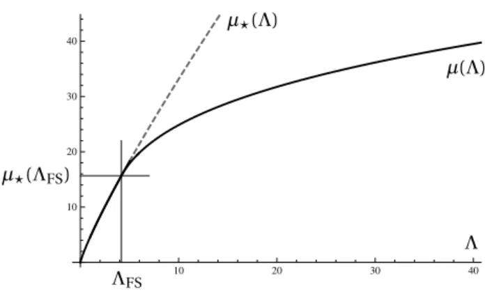
See [37, p. 74] for details. This condition is the symmetry breaking condition of The-orem3. The branch of non-radial solutions bifurcating from Λ = ΛFShas been com-puted numerically in [17] and an example is shown in Fig.1. By construction, we know that Λ 7→ µ(Λ) is increasing, concave, and we read from Theorem3that the non-symmetric branch bifurcates from Λ = ΛFS, and is such that µ(Λ) < µ⋆(Λ) if Λ> ΛFS. This simple scenario explains the symmetry and symmetry breaking prop-erties in (9), but is not generic as we shall see next in the case of more complicated interpolation inequalities.
5.2. Bifurcations, reparametrization and turning points. Let us consider the inter-polation inequality µˆ Rd |u|p |x|bpd x ¶p2 ≤Ca,b,θ µˆ Rd |∇u|2 |x|2a d x ¶θµˆ Rd |u|2 |x|2(a+1)d x ¶1−θ (20) with d ≥ 1, p ∈ (2,2∗) or p = 2∗if d ≥ 3, and θ ∈ (ϑ(p),1] with ϑ(p) := dp−2
2 p . The scaling invariance imposes p = 2d/¡d − 2 + 2(b − a)¢. As proved in [10], the above inequalities hold with a finite constantCa,b,θif a < ac= (d −2)/2, and b ∈ (a+1/2, a+ 1] when d = 1, b ∈ (a,a +1] when d = 2 and b ∈ [a,a +1] when d ≥ 3. Moreover, there exist extremal functions for the inequalities (20) for any p ∈ (2,2∗) and θ ∈ (ϑ(p),1) or θ = ϑ(p) and d ≥ 2, with ac− a > 0 not too large. On the contrary equality is never achieved for p = 2, or a < 0, p = 2∗and d ≥ 3, or d = 1 and θ = ϑ(p,1). The existence of extremal functions has been studied in [16]. We may notice that
0 ≤ ϑ(p) ≤ θ < 1 ⇐⇒ 2 ≤ p ≤ p∗(d,θ) := 2d
d − 2θ< 2
10 20 30 40 10 20 30 40 Λ µ(Λ) µ⋆(Λ) ΛFS µ⋆(ΛFS)
Figure 1:Branches for p = 2.8, d = 5, θ = 1.
With the same conventions as in the previous subsection, the Emden-Fowler change of variables (6) transforms (20) into the Gagliardo-Nirenberg-Sobolev inequality
³ k∇ϕk2L2(C )+ Λkϕk2L2(C ) ´θ kϕk2(1−θ)L2(C ) ≥ µ(θ,Λ)kϕk2Lp(C ) ∀ϕ ∈ H1(C ) (21) on C := R × Sd −1, with Λ = (a − a c)2and µ(θ,Λ) =C−1a,b,θ ¯ ¯Sd −1 ¯ ¯1−2/p. Of course, the case θ = 1 corresponds to the critical case and, consistently, we write µ(1,Λ) = µ(Λ).
For θ < 1, the Euler-Lagrange equation of an extremal function on C is − ∆ϕ +1 θ Ã (1 − θ)k∇ϕk 2 L2(C ) kϕk2L2(C ) + Λ ! ϕ −k∇ϕk 2 L2(C )+ Λkϕk2L2(C ) θ kϕkpLp(C ) ϕp−1= 0. (22) Up to the reparametrization Λ7→ λ =1 θ h (1 − θ)t[ϕ] + Λi where t[ϕ] :=k∇ϕk 2 L2(C ) kϕk2L2(C )
and a multiplication by a constant, an extremal function ϕ for (21) solves (5). In other words, we can use the set of solutions in the critical case θ = 1 to parametrize the solutions corresponding to θ < 1.
Let us start with the symmetric functions. With an evident notation, we define
µ⋆(θ,Λ) as the optimal constant in the inequality corresponding to (21) restricted to symmetric functions, i.e., functions depending only on s ∈ R. If we denote by ϕ⋆,λ the function ϕ⋆,λ(s) = µ1 2p λ cosh ¡p−2 2 p λ s¢−2 ¶p−21
for any λ > 0, then t[ϕ⋆,λ] is explicit and we can parametrize the set©¡Λ,µ⋆(θ,Λ)¢ : Λ> 0ª by ©¡θ λ − (1 − θ)t[ϕ⋆,λ],µ⋆(λ)¢ : λ > 0ª. It turns out that the equation Λ =
θ λ − (1 − θ) t[ϕ⋆,λ] can be inverted, which allows us to obtain λ = Λθ∗(Λ) and get an explicit expression for
µ⋆(θ,Λ) = µ⋆¡Λθ∗(Λ)¢ = µ⋆¡Λθ∗(1)¢ Λθ− p−2
2 p .
According to [13], a Taylor expansion around ϕ⋆,ΛFS shows that for any Λ > ΛθFS,
where
ΛθFS:= θ µFS− (1 − θ) t[uFS], the function ϕ⋆,λwith λ = Λθ
∗(Λ) is linearly unstable, so that µ(θ,Λ) < µ⋆(θ,Λ). The case of non-symmetric functions is more subtle because we do not know the exact multiplicity of the solutions of (5) in the symmetry breaking range. There is a branch of non-symmetric solutions of (22) which bifurcates from the branch of symmetric solutions at Λ = Λθ
FS. This branch has been computed numerically in [17] and a formal asymptotic expansion was performed in a neighborhood of the bifurcation point in [18]. Because of the reparametrization of the solutions of (22) by the solutions of (5), we can use the branch λ 7→ ϕλof non-symmetric extremal functions for λ > ΛFSto get an upper bound of µ(θ,Λ):
µ(θ, Λ) ≤ µ(λ) for any λ > ΛFSsuch that Λ = θ λ − (1 − θ)t[ϕλ].
Actually, we deduce from the branch λ 7→ ϕλof non-symmetric extremal functions an entire branch of non-symmetric solutions of (22) which is parametrized by λ and deduce a parametric curve B :=©¡Λ(λ) := θ λ − (1 − θ)t[ϕλ],µ(λ)¢ : λ > ΛFSª which can be used to bound µ(θ,Λ) from above. If (Λ,µ) ∈ B, we have no proof that ϕλis optimal if µ(λ) < µ⋆(θ,Λ), but at least we know that
µ(λ) =
³
k∇ϕλk2L2(C )+ Λ(λ)kϕλk2L2(C )
´θ
kϕλk2(1−θ)L2(C ) kϕλk−2Lp(C ). Some numerical results are shown in Fig.2.
The formal asymptotic expansion of [18] suggests that there are only two possi-ble generic scenarii:
(i) Either the curve B bifurcates to the right, that is, B is included in the region Λ≥ ΛθFS, and Λ 7→ µ(θ,Λ) is qualitatively expected to be as in Fig.1. We know that this is what happens for θ = 1 and expect a similar behavior for any θ close enough to 1. In this case, the region of symmetry breaking is characterized by the linear instability of the symmetric optimal functions.
(ii) Or the curve B bifurcates to the left. For λ − ΛFS> 0, small enough, the curve
λ 7→¡Λ(λ),µ(λ)¢ satisfies Λ(λ) < Λθ
FSand µ(λ) > µ⋆(θ,Λ(λ)). In that case, the region of symmetry breaking does not seem to be characterized by the linear instability of the symmetric optimal functions and we numerically observe a turning point as in Fig.2(right).
In [19], a priori estimates for branches with θ < 1 were deduced from the known symmetry results (later improved in [26]). This further constrains B and the sym-metry breaking region and determines a lower bound for the value of Λ correspond-ing to a turncorrespond-ing point of the branch. There are many open questions concerncorrespond-ing B
0.5 1.0 1.5 2.0 2.5 3.0 3.5 2 4 6 8 10 2.73 2.74 2.75 2.77 2.78 2.79 2.80 7.82 7.86 7.88 7.90 Λ µ(θ, Λ) µ⋆(θ,Λ) ΛθFS µ⋆(θ,ΛθFS) B B B ΛθFS µ⋆(θ,ΛθFS)
Figure 2:Branches for p = 2.8, d = 5, θ = 0.718. Left: the bifurcation point (Λθ
FS,µ⋆(θ,ΛθFS) is
at the intersection of the horizontal and vertical lines. The area enclosed in the small ellipse is enlarged in the right plot: the branch has a turning point and µ(θ,Λθ
FS) < µ⋆(θ,ΛθFS).
and the set of extremal functions when θ < 1, but at least we can prove that the sym-metry breaking range does not always coincide with the region of linear instability of symmetric optimal functions.
5.3. Symmetry breaking and energy considerations. The exponent ϑ(p) is the ex-ponent which appears in the Gagliardo-Nirenberg inequality
k∇uk2ϑ(p)L2(Rd)kuk 2(1−ϑ(p)) L2(Rd) ≥CGN(p)kuk 2 Lp(Rd) ∀u ∈ H 1(Rd). (23) By considering an extremal function for this inequality and translations, for any p ∈ (2,2∗), one can check that
µ(ϑ(p), Λ) ≤CGN(p) ∀Λ > 0.
Lemma 10. Let d ≥ 2. For any p ∈ (2,2∗), ifCGN(p) < µ⋆(ϑ(p),Λ ϑ(p)
FS ), there exists Λs∈ (0,Λϑ(p)FS ) such that µ(ϑ(p),Λ) = µ⋆(ϑ(p),Λ) if and only if Λ ∈ (0,Λs].
The fact that the symmetry range is an interval of the form (0,Λs] can be de-duced from a scaling argument: see [30,15] for details. The result is otherwise straightforward but difficult to use because the value of CGN(p) is not known ex-plicitly. From a numerical point of view, it gives a simple criterion, which has been implemented in [15]. Moreover, in [18], it has been observed numerically that the conditionCGN(p) < µ⋆(ϑ(p),Λ
ϑ(p)
FS ) is equivalent to a bifurcation to the left as in Fig.2.
For θ and p−2 small enough, the assumption of Lemma10holds. Let us consider the Gaussian test functiong(x) := (2π)−d/4exp(−|x|2/4) in (20) and consider
h(p) :=k∇ gk2θL2(Rd)kgk2(1−θ)L2(Rd) kgk2Lp(Rd) 1 µ⋆(θ,ΛθFS) with θ = ϑ(p).
A computation shows that limp→2+h(p) = 1 and limp→2+
d h
d p(p) < 0. For p − 2 > 0, small enough, we obtain that
CGN(p) ≤ h(p) < µ⋆(θ,ΛθFS).
A perturbation argument has been used in [15] to establish the following result.
Theorem 11. Let d ≥ 2. There exists η > 0 such that for any p ∈ (2,2 + η), µ(θ, Λ) < µ⋆(θ,Λ) if ΛθFS− η < Λ < ΛθFS and ϑ(p) < θ < ϑ(p) + η. 5.4. An open question. The criterion considered in Lemma10is based on energy considerations and provides only a sufficient condition for symmetry breaking. It is difficult to check it in practice, except in asymptotic regimes of the parameters. The formal expansions of the branch near the bifurcation points are based on a purely local analysis, and suggest another criterion: either the branch bifurcates to the right and the symmetry breaking range is characterized by the linear instability of the symmetric optimal functions, or the branch bifurcates to the left, and this is not anymore the case. Is such an observation, which has been made numerically only for some specific values of p, true in general? This seems to be true when θ is close enough to ϑ(p) and at least in this regime we can conjecture that the symmetry
breaking range is not characterized by the linear instability of the symmetric optimal functions if and only if the branch bifurcates to the left.
An additional question, which corresponds to a limiting case, goes as follows. If
θ = ϑ(p), is the range of symmetry determined exactly by the value of the optimal
constant in (23), when it is below µ⋆(θ,Λθ
FS)? Numerically, this is supported by the fact that, in this case, the curve B is monotone increasing as a function of Λ.
In the study of the symmetry issue in (9) and (14), the key tool is the nonlinear flow, which extends a local result (linear stability) to a global result (rigidity). A sim-ilar tool would be needed to answer the conjecture. In the case θ = ϑ(p), it would be crucial to obtain a variational characterization of the non-symmetric solutions in the curve of non-symmetric functions B and a uniqueness result for any given Λ.
REFERENCES
[1] D. BAKRY ANDM. ÉMERY, Hypercontractivité de semi-groupes de diffusion, C. R. Acad. Sci. Paris Sér. I Math., 299 (1984), pp. 775–778.
[2] , Diffusions hypercontractives, in Séminaire de probabilités, XIX, 1983/84, vol. 1123 of Lecture Notes in Math., Springer, Berlin, 1985, pp. 177–206.
[3] , Inégalités de Sobolev pour un semi-groupe symétrique, C. R. Acad. Sci. Paris Sér. I Math., 301 (1985), pp. 411–413.
[4] D. BAKRY, I. GENTIL,ANDM. LEDOUX, Analysis and geometry of Markov diffusion
oper-ators, vol. 348 of Grundlehren der Mathematischen Wissenschaften [Fundamental
Prin-ciples of Mathematical Sciences], Springer, Cham, 2014.
[5] D. BAKRY ANDM. LEDOUX, Sobolev inequalities and Myers’s diameter theorem for an
ab-stract Markov generator, Duke Math. J., 85 (1996), pp. 253–270.
[6] W. BECKNER, Sharp Sobolev inequalities on the sphere and the Moser-Trudinger
[7] A. BENTALEB, Inégalité de Sobolev pour l’opérateur ultrasphérique, C. R. Acad. Sci. Paris Sér. I Math., 317 (1993), pp. 187–190.
[8] M.-F. BIDAUT-VÉRON ANDL. VÉRON, Nonlinear elliptic equations on compact
Rieman-nian manifolds and asymptotics of Emden equations, Invent. Math., 106 (1991), pp. 489–
539.
[9] M. BONFORTE, J. DOLBEAULT, M. MURATORI,ANDB. NAZARET, Weighted fast diffusion
equations (Part I): Sharp asymptotic rates without symmetry and symmetry breaking in Caffarelli-Kohn-Nirenberg inequalities, Kinetic and Related Models, 10 (2017), pp. 33–59.
[10] L. CAFFARELLI, R. KOHN,ANDL. NIRENBERG, First order interpolation inequalities with
weights, Compositio Math., 53 (1984), pp. 259–275.
[11] F. CATRINA ANDZ.-Q. WANG, On the Caffarelli-Kohn-Nirenberg inequalities: sharp
con-stants, existence (and nonexistence), and symmetry of extremal functions, Comm. Pure
Appl. Math., 54 (2001), pp. 229–258.
[12] P. CURIE, Sur la symétrie dans les phénomènes physiques, symétrie d’un champ électrique
et d’un champ magnétique, J. Phys. Theor. Appl., 3 (1894), pp. 393–415.
[13] M. DELPINO, J. DOLBEAULT, S. FILIPPAS, ANDA. TERTIKAS, A logarithmic Hardy
in-equality, Journal of Functional Analysis, 259 (2010), pp. 2045 – 2072.
[14] J. DEMANGE, Improved Gagliardo-Nirenberg-Sobolev inequalities on manifolds with
pos-itive curvature, J. Funct. Anal., 254 (2008), pp. 593–611.
[15] J. DOLBEAULT, M. ESTEBAN, G. TARANTELLO,ANDA. TERTIKAS, Radial symmetry and
symmetry breaking for some interpolation inequalities, Calculus of Variations and Partial
Differential Equations, 42 (2011), pp. 461–485.
[16] J. DOLBEAULT ANDM. J. ESTEBAN, Extremal functions for Caffarelli-Kohn-Nirenberg and logarithmic Hardy inequalities, Proceedings of the Royal Society of Edinburgh, Section:
A Mathematics, 142 (2012), pp. 745–767.
[17] J. DOLBEAULT ANDM. J. ESTEBAN, A scenario for symmetry breaking in
Caffarelli-Kohn-Nirenberg inequalities, Journal of Numerical Mathematics, 20 (2013), pp. 233—249.
[18] , Branches of non-symmetric critical points and symmetry breaking in nonlinear
elliptic partial differential equations, Nonlinearity, 27 (2014), p. 435.
[19] J. DOLBEAULT, M. J. ESTEBAN, S. FILIPPAS, ANDA. TERTIKAS, Rigidity results with
ap-plications to best constants and symmetry of Caffarelli-Kohn-Nirenberg and logarithmic Hardy inequalities, Calc. Var. Partial Differential Equations, 54 (2015), pp. 2465–2481.
[20] J. DOLBEAULT, M. J. ESTEBAN,ANDG. JANKOWIAK, Onofri inequalities and rigidity
re-sults, Discrete and Continuous Dynamical Systems, 37 (2017), pp. 3059–3078.
[21] J. DOLBEAULT, M. J. ESTEBAN, M. KOWALCZYK,ANDM. LOSS, Sharp interpolation in-equalities on the sphere: New methods and consequences, Chinese Annals of
Mathemat-ics, Series B, 34 (2013), pp. 99–112.
[22] , Improved interpolation inequalities on the sphere, Discrete and Continuous Dy-namical Systems Series S (DCDS-S), 7 (2014), pp. 695–724.
[23] J. DOLBEAULT, M. J. ESTEBAN, A. LAPTEV,ANDM. LOSS, One-dimensional Gagliardo–
Nirenberg–Sobolev inequalities: remarks on duality and flows, Journal of the London
Mathematical Society, 90 (2014), pp. 525–550.
[24] J. DOLBEAULT, M. J. ESTEBAN,ANDM. LOSS, Nonlinear flows and rigidity results on com-pact manifolds, Journal of Functional Analysis, 267 (2014), pp. 1338 – 1363.
[25] , Interpolation inequalities, nonlinear flows, boundary terms, optimality and
lin-earization, Journal of elliptic and parabolic equations, 2 (2016), pp. 267–295.
[26] , Rigidity versus symmetry breaking via nonlinear flows on cylinders and Euclidean
[27] , Interpolation inequalities on the sphere: linear vs. nonlinear flows (inégalités
d’interpolation sur la sphère : flots non-linéaires vs. flots linéaires), Annales de la faculté
des sciences de Toulouse Sér. 6, 26 (2017), pp. 351–379.
[28] J. DOLBEAULT, M. J. ESTEBAN, M. LOSS,ANDM. MURATORI, Symmetry for extremal func-tions in subcritical Caffarelli–Kohn–Nirenberg inequalities, Comptes Rendus
Mathéma-tique, 355 (2017), pp. 133 – 154.
[29] J. DOLBEAULT, M. J. ESTEBAN, M. LOSS,ANDG. TARANTELLO, On the symmetry of
ex-tremals for the Caffarelli-Kohn-Nirenberg inequalities, Advanced Nonlinear Studies, 9
(2009), pp. 713–727.
[30] , On the symmetry of extremals for the Caffarelli-Kohn-Nirenberg inequalities, Adv. Nonlinear Stud., 9 (2009), pp. 713–726.
[31] J. DOLBEAULT ANDM. KOWALCZYK, Uniqueness and rigidity in nonlinear elliptic
equa-tions, interpolation inequalities, and spectral estimates. To appear in Annales de la
Fac-ulté de Sciences de Toulouse, Mathématiques, 2017.
[32] J. DOLBEAULT, M. MURATORI,ANDB. NAZARET, Weighted interpolation inequalities: a
perturbation approach, Mathematische Annalen, (2016), pp. 1–34.
[33] J. DOLBEAULT ANDG. TOSCANI, Nonlinear diffusions: Extremal properties of Barenblatt
profiles, best matching and delays, Nonlinear Analysis: Theory, Methods & Applications,
(2016), p. to appear.
[34] V. FELLI ANDM. SCHNEIDER, Perturbation results of critical elliptic equations of
Caffa-relli-Kohn-Nirenberg type, J. Differential Equations, 191 (2003), pp. 121–142.
[35] B. GIDAS ANDJ. SPRUCK, Global and local behavior of positive solutions of nonlinear
elliptic equations, Comm. Pure Appl. Math., 34 (1981), pp. 525–598.
[36] V. P. IL’IN, Some integral inequalities and their applications in the theory of differentiable
functions of several variables, Mat. Sb. (N.S.), 54 (96) (1961), pp. 331–380.
[37] L. D. LANDAU ANDE. LIFSCHITZ, Physique théorique. Tome III: Mécanique quantique.
Théorie non relativiste. (French), Deuxième édition. Translated from russian by E.
Gloukhian. Éditions Mir, Moscow, 1967.
[38] J. R. LICOIS ANDL. VÉRON, A class of nonlinear conservative elliptic equations in
cylin-ders, Ann. Scuola Norm. Sup. Pisa Cl. Sci. (4), 26 (1998), pp. 249–283.
[39] C. E. MUELLER ANDF. B. WEISSLER, Hypercontractivity for the heat semigroup for
ultra-spherical polynomials and on the n-sphere, J. Funct. Anal., 48 (1982), pp. 252–283.
[40] G. SAVARÉ ANDG. TOSCANI, The concavity of Rényi entropy power, IEEE Trans. Inform. Theory, 60 (2014), pp. 2687–2693.
[41] G. TOSCANI, Rényi Entropies and Nonlinear Diffusion Equations, Acta Appl. Math., 132 (2014), pp. 595–604.
J. DOLBEAULT& M.J. ESTEBAN: CEREMADE, CNRS, UMR 7534, Université Paris-Dauphine, PSL Research University, Place de Lattre de Tassigny, F-75016 Paris, France.
E-mail:[email protected],[email protected]
M. LOSS: School of Mathematics, Skiles Building, Georgia Institute of Technology, Atlanta GA 30332-0160, USA.E-mail:[email protected]