HAL Id: pastel-00822242
https://pastel.archives-ouvertes.fr/pastel-00822242
Submitted on 14 May 2013
HAL is a multi-disciplinary open access archive for the deposit and dissemination of sci-entific research documents, whether they are pub-lished or not. The documents may come from teaching and research institutions in France or abroad, or from public or private research centers.
L’archive ouverte pluridisciplinaire HAL, est destinée au dépôt et à la diffusion de documents scientifiques de niveau recherche, publiés ou non, émanant des établissements d’enseignement et de recherche français ou étrangers, des laboratoires publics ou privés.
A window on stochastic processes and gamma-ray
cosmology through spectral and temporal studies of
AGN observed with H.E.S.S.
Jonathan Biteau
To cite this version:
Jonathan Biteau. A window on stochastic processes and gamma-ray cosmology through spectral and temporal studies of AGN observed with H.E.S.S.. High Energy Astrophysical Phenomena [astro-ph.HE]. Ecole Polytechnique X, 2013. English. �pastel-00822242�
A window on stochastic processes
and γ-ray cosmology through
spectral and temporal studies
of AGN observed with H.E.S.S.
Jonathan Biteau
Soutenue le 22 f´evrier 2013, devant le jury compos´e de : Martin Lemoine, Pr´esident
Fr´ederic Daigne, Rapporteur
John Quinn, Rapporteur
R´egis Terrier, Examinateur
Christian Stegmann, Examinateur Berrie Giebels, Directeur de th`ese
Preamble 1
Pr´eambule 3
Acronyms list 7
Chapter 1. Very high energy blazars 11
1.1. Quasars, AGN and blazars 11
1.1.1. Half a century of quasar astronomy 11
1.1.2. The components of an AGN 19
1.2. Jetted emission of blazars 27
1.2.1. Transferring the jet energy to particles 27 1.2.2. Radiation of the accelerated particles 33 1.3. Observing blazars at high and very high energies 42 1.3.1. γ-ray astronomy in space and on Earth 42
1.3.2. Universe transparency to γ rays 49
Bibliography 57
Chapter 2. AGN targeted with H.E.S.S. 63
2.1. Targeting AGN with H.E.S.S. 63
2.1.1. The H.E.S.S. experiment 63
2.1.2. Observation strategy 70
2.2. AGN observed at VHE 77
2.2.1. Detected AGN 77
2.2.2. Signals compatible with background fluctuations 81 2.3. The blazars 1ES 1312-423 and SHBL J001355.9-185406 88
2.3.1. H.E.S.S. data 89
2.3.2. Broad band SEDs 96
Bibliography 105
Chapter 3. Spectral studies: first EBL measurement at VHE 111
3.1. Spectral modelling and datasets 111
3.1.1. Intrinsic spectrum 111
3.1.2. EBL absorption 113
3.1.3. Datasets 116
3.2. Analysis and discussion 118
3.2.1. Spectral analysis 118
3.2.2. Discussion of the detection 129
3.3. Intrinsic spectra of H.E.S.S. blazars 134
3.3.1. Spectral analysis 134
3.3.2. Multi-wavelength overview 137
Bibliography 141
Chapter 4. Variability - minijets-in-a-jet statistical model 143 4.1. The dramatic outbursts of PKS 2155-304 144
4.1.1. Temporal properties 145
4.1.2. Statistical properties 147
4.1.3. Spectral variability 150
4.1.4. Fourier properties 152
4.2. Modelling of the outbursts 157
4.2.1. The additive/multiplicative dilemma 158
4.2.2. The minijets-in-a-jet statistical model 164 4.2.3. Telegraph process and spectral assumption 171
Bibliography 181
Chapter 5. Perspectives 185
5.1. Short-term and mid-term instrumental prospects 185 5.1.1. The low-energy threshold of H.E.S.S. II 185
5.1.2. The large effective area of CTA 188
5.1.3. AGN science with current and next generation IACT 194
5.2. EBL-dependent prospects 198
5.2.1. Measuring redshifts: toward cosmological constraints 199
5.2.2. Refining the EBL measurement 200
5.3. Variability studies 203
5.3.1. Below the minute time-scale? 203
5.3.2. Long-term monitoring 208
Conclusion 217 ´
Epilogue 221
Appendix A. Reliability of the reconstruction at large offset 227
A.1. Selection of the runs 227
A.2. Reconstruction of the spectrum 229
Appendix B. Appendix of the EBL study 233
B.1. Cross checks and systematic uncertainties 233
B.1.1. Analysis chain 233
B.1.2. Intrinsic model 236
B.1.3. Energy scale and EBL model 238
B.1.4. Energy range covered 239
B.1.5. A glimpse at the wiggle 241
B.2. Intrinsic spectral parameters 244
B.3. Lists of runs 246
Appendix. Bibliography 251
Appendix C. Instrumental uncertainty on the PSD 253
C.1. Estimating the PSD of one realization 253
C.2. “Naive” propagation of the uncertainties 254
C.3. Using a Gaussian field 255
C.4. Simulation check 258
Appendix. Bibliography 261
The second half of the twentieth century saw tremendous techni-cal and technologitechni-cal developments led by world-wide collaborations of scientists and engineers. The scientific horizon expanded with, among others, the birth of the first large accelerators, the opening up of the sky from radio wavelengths to γ rays, and the advent of computing facilities. The greatest achievements of modern physics induced by these developments probably concern our understanding of the Uni-verse, which, under the current state of the art, evolved from a primor-dial hot and dense plasma of elementary particles to form the stars and the galaxies, surrounded by dark matter and dark energy.
Among the most important of the fields that emerged is high-energy astrophysics, which aims at applying the laws of physics to the extreme and violent Universe in order to constrain its constituents and discover new laws. High-energy astrophysics is based on the measurements per-formed in X-ray astronomy, γ-ray astronomy, as well as on the studies of neutrinos, cosmic rays and gravitational waves. These observations make possible research on properties of matter under physical condi-tions that cannot be achieved in the laboratory and on distances and time-scales that by far exceed the human limitations. The questions raised by this field are at the cross-roads of astrophysics, cosmology, particle physics and fundamental physics, focussing on:
· the origin and nature of (extra)galactic cosmic rays, · the search for dark matter particle candidates, · the search for Lorentz invariance violation,
· the environment of black holes, neutron stars, supernovae, · the particle acceleration in these astrophysical environments, · the search for astrophysical neutrinos and gravitational waves, · the nature of enigmatic transients (gamma-ray bursts, flares),
· the cosmological backgrounds and magnetic fields.
Parts of these vast questions are elucidated by experiments led by international collaborations. French institutes are particularly involved in experiments such as the γ-ray satellite Fermi, the ground based γ-ray telescope H.E.S.S. and the future array CTA. Other messengers than photons are under study, with neutrinos for ANTARES, cosmic-rays for AUGER and CODALEMA, and gravitational waves for VIRGO and the planned LISA. Research on the content and constituents of the Universe is carried out by AMS-02 for anti-matter, Edelweiss for dark matter particle candidates, as well as SCP, SNLS, SNFactory, Planck and the planned Snap and EUCLID for the density of dark matter and dark energy.
The studies developed in this manuscript exploit the results of Fermi and primarily of H.E.S.S. on phenomena occurring in the vicin-ity of the most massive black holes known in the Universe, hosted in active galactic nuclei. I purposely focus on these objects, called AGN, quasars or blazars as appropriate, and do not mention the other cosmic accelerators, which are now sufficiently numerous at high energy (tens of MeV up to hundreds of GeV) and very high energies (hundreds of GeV up to tens of TeV) to deserve a dedicated discussion. I describe in the first chapter the present state of the scientific knowledge regarding AGN. I then expose the characteristics of H.E.S.S. and explain how they can be used to discover new sources, such as the faint blazars 1ES 1312-423 and SHBL J001355.9-185406, detections which I have directly contributed to. The third chapter develops an important step in the advent of γ-ray cosmology, with the first detection of a cosmo-logical background using very high energy γ rays from blazars. I study in chapter 4 one of the most striking property of blazars, their extreme variability, and I develop a model based on relativistic beaming and the generalized central limit theorem to explain their flux as a stochastic process. Based on these results and models, I finally summarize the sci-entific perspectives of the future ground-based instruments H.E.S.S. II and CTA.
La seconde moiti´e du vingti`eme si`ecle a connu des d´eveloppements techniques et technologiques extraordinaires, men´es de concert par des collaborations internationales de chercheurs et d’ing´enieurs. L’horizon de la science s’en est vu ´etendu, avec, entre autres, la naissance des premiers grands acc´el´erateurs, l’ouverture de nouvelles fenˆetres spec-trales sur le ciel de la radio jusqu’aux rayons γ et l’av`enement des grandes structures de calcul num´erique. Les plus grandes avanc´ees de la physique qui ont r´esult´e de ces progr`es concernent tr`es certainement notre compr´ehension de l’Univers. Ce dernier, en l’´etat actuel des con-naissances, a ´evolu´e depuis l’´etat de plasma dense et chaud de particules ´el´ementaires pour former par la suite les ´etoiles et les galaxies, dans un milieu essentiellement constitu´e de mati`ere noire et d’´energie noire.
L’astrophysique des hautes ´energies est un des principaux domaines ayant ´emerg´e. Elle tente d’appliquer les lois de la physique `a l’Univers violent, pour contraindre ses constituants et d´ecouvrir de nouvelles lois. Elle exploite les mesures r´ealis´ees en astronomie X et en astronomie γ, ainsi que les ´etudes de neutrinos, de rayons cosmiques et d’ondes grav-itationnelles. `A l’aide de ces observations, il devient possible d’´etudier les propri´et´es de la mati`ere dans des conditions inaccessibles sur Terre et sur des distances et des ´echelles de temps que l’Homme con¸coit dif-ficilement. Les questions que soul`eve ce domaine sont `a la crois´ee des chemins entre astrophysique, cosmologie, physique des particules et physique fondamentale. En particulier, sont ´etudi´es :
· l’origine et la nature des rayons cosmiques (extra)galactiques, · la recherche d’hypoth´etiques particules de mati`ere noire, · la recherche de violation d’invariance de Lorentz,
· l’environnement des trous noirs, des ´etoiles `a neutrons et des supernovae,
· l’acc´el´eration de particules en environnement astrophysique, · la recherche de neutrinos d’origine astrophysique et d’ondes
gravitationnelles,
· la nature des ´ev´enements transitoires tels que les sursauts gamma ou les ´eruptions astrophysiques,
· les fonds diffus et champs magn´etiques cosmologiques. Des ´el´ements de r´eponse `a ces vastes questions ne peuvent ˆetre trouv´es qu’`a l’´echelle de collaborations internationales. Les instituts fran¸cais s’impliquent tout particuli`erement dans des exp´eriences telles que le satellite γ Fermi, le t´elescope γ H.E.S.S. et le futur grand r´eseau de t´elescopes CTA. D’autres messagers que les photons pourraient aussi ˆetre mis `a profit, tels que les neutrinos d’ANTARES, les rayons cos-miques d’AUGER et de CODALEMA et les ondes gravitationnelles de VIRGO et du futur LISA. Une contribution `a l’´etude du contenu et des constituants de l’Univers est enfin apport´ee par la France dans des exp´erience telles qu’AMS-02 pour l’anti-mati`ere, Edelweiss pour les particules de mati`ere noire, mais aussi SCP, SNLS, SNFactory, Planck et les futurs Snap et EUCLID, pour l’´etude des densit´es de mati`ere et d’´energie noires.
Les travaux d´ecris dans ce manuscrit tirent profit des observations de Fermi et surtout de H.E.S.S. Ils portent sur les ph´enom`enes se d´eroulant au voisinage des trous noirs les plus massifs que l’on con-naisse dans l’Univers, qui sont lov´es au sein des noyaux actifs de galax-ies. Je me limite volontairement `a l’´etude de ces objets, qu’on appelle AGN, blazars ou quasars selon les cas, et je ne fais pas mention des autres acc´el´erateurs cosmiques. Ces derniers sont maintenant suffisam-ment nombreux `a haute ´energie (quelques dizaines de MeV jusqu’`a des centaines de GeV) et `a tr`es haute ´energie (quelques centaines de GeV jusqu’`a des dizaines de TeV) pour m´eriter une discussion sp´ecifique. Je d´ecris dans le premier chapitre l’´etat actuel des connaissances sur les AGN. J’expose ensuite les caract´eristiques de H.E.S.S. et montre comment elle peuvent servir la d´ecouverte de nouvelles sources, telles que les blazars de faible luminosit´e 1ES 1312-423 et SHBL J001355.9-185406, d´et´ections auxquelles j’ai directement contribu´e. Le troisi`eme chapitre expose une ´etape marquante dans l’av`enement de la cosmolo-gie γ : la premi`ere d´etection d’un fond diffus cosmologique `a l’aide
de rayons γ de tr`es haute ´energie provenant de blazars. J’´etudie au chapitre 4 une des propri´et´es les plus surprenantes des blazars : leur extrˆeme variabilit´e. Cela me permet de construire un mod`ele combi-nant focalisation relativiste et th´eor`eme de la limite centrale g´en´eralis´e, et d’identifier le flux des blazars `a un processus stochastique. `A l’aide de ces r´esultats et de ces mod`eles, j’envisage enfin quelques unes des per-spectives des prochaines g´en´erations de t´elescope γ, `a savoir H.E.S.S. II et CTA.
· ACD: Anti-coincidence dome · ADC: Analogic to digital convertor · AGN: Active galactic nucleus · ARS: Analogic ring sampler · BLR: Broad-line region
· BLRG: Broad-line radio galaxy · C.U.: Crab unit
· CIB: Cosmic infrared background · CLT: Central limit theorem
· CMB: Cosmic microwave background · COB: Cosmic optical background · DFT: Discrete Fourier transform · dof: number of degrees of freedom
· EBL: Extragalactic background light (the COB and the CIB in this manuscript)
· ECAL: Electromagnetic calorimeter · EDF: Electron distribution function
· ELP: Log parabola with an exponential cut off · EPWL: Power law with an exponential cut off · FFT: Fast Fourier transform
· FoV: field of view
· FR I, FR II: Fanaroff-Riley galaxy of type I and II
· FR08: EBL model of Franceschini et al., 2008 (baseline in this manuscript)
· FSRQ: Flat spectrum radio quasar · FT: Fourier transform
· GCLT: Generalized central limit theorem
· HDMVA: Multivariate analysis in Ohm et al., 2009 · HE: High energy (20 MeV < E < 100 GeV)
· HSP, HBL: High frequency synchrotron peaked blazars (resp. BL Lac objects)
· IACT: Imaging atmospheric Cherenkov telescope
· IBL, ISP: Intermediate frequency synchrotron peaked blazars (resp. BL Lac objects)
· LBL, LSP: Low frequency synchrotron peaked blazars (resp. BL Lac objects)
· LP: Log parabola
· LST: Large size telescope of CTA · MST: Medium size telescope of CTA · NLR: Narrow-line region
· NLRG: Narrow-line radio galaxy
· OVV: Optically violently variable (∼FSRQ) · pdf: Probability density function
· PM: Photo multiplier
· PMVA: Multivariate analysis in Becherini et al., 2011 · PSD: Power spectral density
· PSF: Point spread function · PWL: Power law
· QSO: Quasi stellar object (∼RQQ) · RLQ: Radio loud quasar
· RQQ: Radio quiet quasar
· SED: Spectral energy distribution
· SEPWL: Power law with a super-exponential cut off · SSC: Synchrotron self Compton
· SST: Small size telescope of CTA · Sy: Seyfert Galaxy
· TS: Test statistics
Very high energy blazars
1.1. Quasars, AGN and blazars
The year 1963 is one of the landmarks of extragalactic astronomy, with the discovery that quasi-stellar radio sources (quasars) are ex-tragalactic objects. This triggered the meeting of astronomers, as-trophysicists and physicists from general relativity in the first Texas Symposium, planting the seeds of the field of relativistic astrophysics. I adopt in the following an historical approach to describe the var-ious sub-classes of active galactic nuclei (AGN) and discuss the unifi-cation scheme that has emerged during the past fifty years. A more extensive discussion can be found in the excellent books of Kembhavi & Narlikar (1999) and Krolik (1999).
1.1.1. Half a century of quasar astronomy
Up to the end of the ’20s, astronomical observations were performed exclusively in the optical band. The existence of extragalactic sources was established in 1924, with the work of Edwin Hubble (among oth-ers). In the beginning of the ’40s, Carl Seyfert performed the first sys-tematic spectroscopic study of spiral galaxies with bright nuclei (Seyfert 1943), now called AGN. The ’40s also saw the pioneering work of Karl Jansky and Grote Reber, who performed the first observations of our galaxy in the radio band. In the ’50s, scientists and engineers who had worked on radars during World War II took up the work of Jansky and Reber and discovered the first radio galaxies, such as the nearby Centaurus A, M 87 or Cygnus A. The emission of these objects was found to be polarized, indicating the non-thermal synchrotron origin of the emission (cf. Sect. 1.2.2.1).
1.1.1.1. The year 1963: the birth of quasar astronomy and relativistic astrophysics
The first quasars were discovered at the end of the ’50s. Their name originates from the acronym QSRS, for quasi-stellar radio sources, be-cause these objects have a very small angular extension and thus appear point like, as would stars. The nature of their astrophysical counter-parts remained puzzling, but the collaboration of radio and optical astronomers created the breeding ground for the major discoveries of 1963. Quoting Maarteen Schmidt (Schmidt 1990):
“The puzzle was suddenly resolved in the afternoon of February 5, 1963, while I was writing a brief article about the optical spectrum of 3C 273. Cyril Hazard had written up the occultation results for publica-tion in Nature and suggested that the optical observapublica-tions be published in an adjacent article. While writing the manuscript, I took another look at the spectra. I noticed that four of the six lines in the photo-graphic spectra showed a pattern of decreasing strength and decreasing spacing from red to blue. For some reason, I decided to construct an energy-level diagram based on these lines. I must have made an error in the process which seemed to contradict the regular spacing pattern. Slightly irritated by that, I decided to check the regular spacing of the lines by taking the ratio of their wavelengths to that of the nearest line of the Balmer series. The first ratio, that of the 5630 line to H-β, was 1.16. The second ratio was also 1.16. When the third ratio was 1.16 again, it was clear that I was looking at a Balmer spectrum redshifted by 0.16.”
A redshift of 0.16 indicated the extragalactic origin of 3C 273 and with an optical magnitude of 13, the luminosity of the object had to be tremendous! When, a few minutes latter, Maarteen Schmidt talked in the hallway with J. Greenstein, who was working on the spectrum of 3C 48, they immediately realized that the spectrum of the latter object corresponds to a redshift of 0.37, a gigantic cosmological distance for the epoch. One should recall that the usual galaxies that were known by then ranged up to a redshift of∼ 0.2. The four consecutive articles about these two quasars that were published in Nature (Hazard et al. 1963; Schmidt 1963; Oke 1963; Greenstein 1963) immediately caught the eye of theoreticians.
Schucking (1989) describes how, a few months later, I. Robinson (mathematician) and himself (from general relativity) were sitting by
a pool on a hot day of July, near Dallas, Texas, talking about the dull summer. L. Marshall, head of the Office of Scientific Personnel in the centre of gravity in Austin, suggested: “Look you fellows. You’ve got a golden opportunity... a new division and new territory to branch into... Why don’t you organize a little conference?”. They passed the next days thinking about it until E. Schucking said: “You know, there are some new astronomical objects, observed by telescopes, and nobody knows quite what they are... Why don’t we hold a conference on the subject?”
The conference was held in December 1963 and a long series of “Texas Symposia” (originally financed by the university of Texas) was born, together with the field of relativistic astrophysics. Greenstein gave the main talk on 3C 273. Another major contribution to the conference was the newly discovered metric of R. Kerr (Kerr 1963), who studied the rotation of black holes, which happens to be one of the greatest energy reservoirs in the Universe. The self collapse of massive objects, which can lead to black hole formation as discussed in the following, was also pointed out a couple of months before by Hoyle & Fowler (1963), who realized that for large masses M , the thermonuclear energy∝ M must be dominated by the gravitational energy ∝ M2.
1.1.1.2. From quasars to the birth of blazars in 1978 The end of the ’60s saw the advent of X-ray astronomy with the detection of 3C 273, M 87 and Centaurus A (Friedman & Byram 1967; Bowyer et al. 1970), showing that quasars share properties in common with radio galaxies. In the beginning of the ’70s, the first very long baseline interferometry observations were performed, enabling angular resolution below the milli-arcsec. Observations of the quasars 3C 273 and 3C 279 revealed structures moving with apparent speeds larger than the speed of light by factors of at least 2 and 3 (Cohen et al. 1971) and even by a factor as large as 10 according to Whitney et al. (1971). This apparent superluminal speed had been predicted by Rees (1966) with simple geometrical arguments, given that the true speed of the object is larger than 0.71c (= c/√2) and that the motion is almost co-linear with the line of sight.
The idea of a high-velocity emitting region moving toward the ob-server was recycled in 1978 for a different class of radio sources during the Pittsburgh Conference on BL Lac objects (Wolfe 1978). These
sources are named after BL Lacertae, originally thought to be a vari-able star in the constellation of Lacerta and later associated with a radio source (Schmitt 1968). BL Lacs usually show faint lines with respect to their non-thermal emission, complicating the measurement of their redshifts. One of the conclusions of the conference was the great resemblance between BL Lacs and flat spectrum radio quasars (FSRQs, also called OVVs for optically violently variables), the two classes exhibiting polarized and highly variable emission. The differ-ence between these objects lies in the strong emission lines observed in FSRQs, with an equivalent width1 of EW > 5˚A. The after-dinner speaker of this conference, Ed Spiegel, created the name “blazar” to unite these two classes of object.
During this founding conference, Blandford & Rees (1978) explained that the continuum observed in blazars probably arose, as in radio galaxies, from synchrotron radiation. The fast variability, however, should imply a tiny emitting region invoking what is now known as the causality argument: the emission of a region of size R can not vary on time scales shorter than the time needed to cross the region at the speed of light, i.e. R/c. The high luminosity observed from such a small region would result in large synchrotron self absorption (see Sect. 1.2.2.1) and large electron scattering that would imply no polar-ization. The problem can be resolved by imposing a relativistic boost on the emitting region (see Sect. 1.1.2.1), which shortens the observed time scales and enhances the emission for a direction of motion in close alignment with the line of sight.
The late ’70s also saw the advent of charge coupled device (CCD) cameras, which enabled the resolution, in the optical band, of the cores of nearby elliptical radio galaxies such as M 87. The bright core emis-sion, as shown in Fig. 1, serves as a natural bridge with the nuclei of Seyfert galaxies, all of them belonging to the class of AGN.
Large X-ray surveys began in the ’80s, in particular with the Ein-stein observatory (HEAO-2, Giacconi et al. 1979). The common prop-erties of radio galaxies, Seyfert galaxies, quasars and blazars progres-sively led to the conclusion that they must host an AGN, powered 1The equivalent width (EW) of a line is defined as the integral under the curve |Fλ− F0|/F0, where F0is the flux of the continuous (non-thermal) emission and Fλ the total flux (line + continuum). This quantity thus highly depends on the state of a variable source (on F0), a high state reducing EW. FSRQs in high states have thus the same properties as BL Lac objects.
Figure 1. Luminosity profile of M87 showing that the emission is dominated by the bright active nucleus be-low a hundred light years. Extracted from Kembhavi & Narlikar (1999).
by gravitational energy, which can outshine the emission of the whole galaxy, be it spiral (for Seyferts) of elliptical (for the others).
1.1.1.3. The properties of AGN
In their classic book, Burbidge & Burbidge (1967) list the crite-ria (established by Maarten Schmidt) that an object must fulfil to be identified as a quasar. These criteria are compared in Table 1 with the “ingredients” that compose an AGN, taken from in the menu of Krolik (1999). Apart from radio emission, which is now known to character-ize a minority of AGN, the properties initially defining quasars largely describe the entire class of AGN. These are extragalactic sources (i.e. have what was considered a large redshift in the ’60s) and are point-like objects on optical photographic plates. They used to be selected
by their large UV flux that, being of non-thermal origin, differenti-ates them from stars. This technique has been successful for discov-ering quasars with a rather weak radio emission, so-called radio-quiet quasars (RQQ, also QSO), which distinguishes them from the radio-loud quasars (RLQ) that were originally discovered.
More generally, AGN have broad-band spectra that can extend from radio wavelengths up to γ rays for the most energetic objects. Their luminosity can range from 1% up to 104 times that of a typical galaxy2. Most of the AGN, but not all of them (e.g. BL Lac objects), have prominent emission lines, in contrast with stars or galaxies that usually exhibit weak absorption lines. The most common lines are the Ly α and the Balmer series of hydrogen (originally used for 3C 273), but also the doublet at 1549˚A of CIV, the line at 5007˚A of OIII and the Kα X-ray line of iron at 6.4 keV.
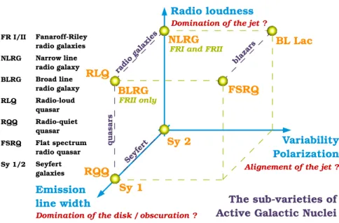
Unlike normal galaxies, AGN are variable sources. The usual vari-ation is on the order of ∼ 10% on the ∼year time scale and their emission is weakly polarized (linear polarization on the order of 1%), but strongly enough to distinguish them from stars or galaxies (typ-ically 0.5% linearly polarized). A minority are strongly variable and much more polarized (∼ 10% in linear polarization), most of these being bright blazars. Following the schematic arrangement of Krolik (1999), one can distinguish the sub-varieties of AGN as a function of their radio loudness, of the width of their emission lines and of their variability/polarization, as in Fig. 2.
I already mentioned BL Lacs and FSRQs, the two sub-classes of blazars, which are radio-loud, variable, polarized objects. They are distinguished by the widths of their emission lines with those of the BL Lacs usually being weak to non-existant and those of FSRQs being stronger and broader. Seyfert (Sy) galaxies, which are non-variable unpolarized radio-quiet objects, can also be divided into two classes based on the width of their emission lines with type 2 and type 1 objects having narrow and broad lines, respectively. Their radio-loud equivalents are the narrow and broad lines radio galaxies (NLRG and BLRG). Note that, while BLRG and Sy 1 have particularly bright optical emission, their optically faint equivalents are the so-called RLQ and RQQ.
1.1. QUASARS, A GN AND BLAZARS 17
for quasars (’60s) for AGN (’90s) in AGN
Large redshift Extragalactic All If measurable redshift
Star-like object Very small angular size Many Wavelength dependent
Large UV flux &Galactic luminosity Many Malmquist bias
Broad-band continuum Most
Broad emission lines Strong emission lines Most Sometimes narrow
Variable Variable, weakly polarized Most ∼ 1% linear polarization
Strongly variable, polarized Minority Usually radio and γ rays
Radio emission Radio emission Minority Mostly very weak
Sometimes extended Table 1. Comparison of the criteria of M. Schmidt to select quasars with the ingredients of J. Krolik that compose an AGN.
Figure 2. Principal sub-varieties of AGN, ordered as a function of their relative power in the radio band, of the width of their emission lines and of their variability and polarization. Adapted from Krolik (1999).
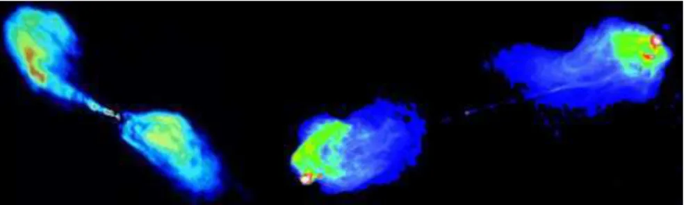
A common classification of radio galaxies was established by Fa-naroff & Riley (1974) and this is still widely used today. FR I galax-ies are characterized by a distance between their two brightest spots smaller than half the size of the whole structure and FR II have more distant brightest spots. As shown in Fig. 3 with Centaurus A and Cygnus A, FR II galaxies tend to have more collimated and fainter jets than FR Is and exhibit very bright terminal hot spots. This morpho-logical distinction is remarkably correlated with the radio luminosity of the object, FR IIs being brighter than FR Is. Ledlow & Owen (1996) showed that the radio luminosity that divides the two classes roughly goes as the square of the optical luminosity of the host, indicating an apparent link between the host and the giant jetted structures on Mpc
scales3. When resolved, the jets of FSRQs mostly exhibit FR II-like structures while those of BL Lacs can belong to either class (Ledlow & Owen 1996; Antonucci 2011).
Figure 3. Left: FR I radio galaxy Centaurus A. Right: FR II radio galaxy Cygnus A.
1.1.2. The components of an AGN
A global picture of the various ingredients necessary to understand the sub-classes of AGN emerged in the ’90s. I discuss these ingredients and the current unification scheme in the following sections.
1.1.2.1. The jetted emission
The large scale Mpc structures observed in radio galaxies such as Centaurus A and Cygnus A, and also the jet of the FR I M 87 in the optical band (reported since the ’20s) point back to their central source of power down to the smallest scales. Very long baseline interferometry has revealed since the ’70s the continuity of jets down to the kpc and pc scales, but the sub-pc scale, presumably where the most energetic radiation is emitted, usually remains un-resolved. Note however that, recently, the emission of M 87 has been resolved in the radio band down to 5 mpc (Doeleman et al. 2012).
The discovery of superluminal motion (introduced in Sect. 1.1.1.2) in the jets of the FSRQs 3C 273 and 3C 279 by Cohen et al. (1971) and Whitney et al. (1971), which had been theorized by Rees (1966), can be be explained by arguments that are purely geometric, as shown
Figure 4. Schematic view of the motion of an emit-ting region along a direction at angle θ from the line of sight. The signal emitted at ti,1 (resp. ti,2) travels for d1/c (resp. d2/c) before arriving at t1 (resp. t2). A displacement of L is observed between t1 and t2, for an effectively travelled distance of H.
in Fig. 4. The apparent velocity vapp is given by Eq. (1.1): (1.1) vapp = L t2− t1 = L (ti,2+dc2)− (ti,1+dc1) = L (ti,2− ti,1)−d1−dc 2 where the only hypothesis is that the signal travels at the speed of light c. The “true” velocity of the emitting region is vi = H/(ti,2−ti,1). Then using Eq. (1.1), the apparent velocity is:
(1.2) vapp = H sin θ H/vi− H cos θ/c = visin θ 1−vi c cos θ
Calling β = vi/c, and using t = tan θ/2, Eq. (1.1) can be re-written with standard trigonometry vapp/c = 2βt/£(1 − β) + (1 + β)t2¤, so that after a bit of algebra:
where γ = 1/p1 − β2 is the Lorentz factor of the region. The left hand term is positive and the equation in t admits at least one solution if β/k≥ 1/γ. Superluminal motion vapp≥ c (i.e. k ≥ 1) is then possible as long as γβ ≥ vapp/c. A direct consequence of the previous equa-tion is γ≥ vapp/c, which proves that, even for moderate superluminal motions, the true velocity is relativistic.
This relativistic motion yields anisotropic emission. It also en-hances the energy of the photons and the intensity of the radiation when the region is moving toward the observer. The textbook deriva-tion of this effect, called the relativistic Doppler effect, is based on the velocity transformation. I propose here a simple framework based on the transformation of the energy of an emitted photon. I assume isotropic emission at the energy Eiso in the emitting region frame (orange cloud in Fig. 4) and I call the associated four-momentum [Eiso, px, iso, py, iso, pz, iso]. The observer receives photons with an en-ergy E in his own rest frame. Since only the photons travelling along the line of sight are received, the observed four-momentum can be writ-ten [E, px = E, py = 0, pz = 0], where x is the direction of the line of sight (I adopt here the convention c = 1). These two four-momenta are related with a Lorentz boost γ of the emitting region and a rotation of θ from the direction of motion, i.e.:
E E 0 0 = 1 cos θ sin θ − sin θ cos θ 1 γ γβ γβ γ 1 1 Eiso px, iso py, iso pz, iso or inversely Eiso px, iso py, iso pz, iso = γ −γβ −γβ γ 1 1 1 cos θ − sin θ sin θ cos θ 1 E E 0 0 which reads: (1.4)
[Eiso, px, iso, py, iso, pz, iso] = [γE(1− β cos θ), γE(cos θ − β), E sin θ, 0] The time-like component can be used to define the Doppler factor δ as the ratio of the received and emitted energies:
(1.5) δ = E
Eiso
= 1
The Doppler factor is thus the quantity by which the energy is enhanced in the observer frame and its maximal value is δmax= 1/γ(1− β) ∼ 2γ (where ∼ corresponds to the ultra-relativistic limit β → 1). With the energy being enhanced by δ, so too is the frequency. Time, which is the inverse of frequency, is then contracted by a factor δ.
The Doppler factor also affects the beaming of the radiation. In-deed, following Eq. (1.4), px, iso ≥ 0 corresponds to cos θ ≥ β, i.e. 1−θ2/2≥ 1−γ−2/2 in the ultra-relativistic limit, which reads θ≤ 1/γ. Thus the front hemisphere of the emission is transformed into a cone of half-opening angle θ = 1/γ.
Finally, the effect on the specific intensity Iν per unit solid angle can be derived, as in Rybicki & Lightman (1979), using what could be called a relativistic Liouville’s theorem, i.e. the invariance of the number of particles per phase volume dN /d3xd3p under a Lorentz transformation. Since the energy density per unit solid angle uνdν is linked to the specific intensity via uνdν = Iνdν/c and can easily be expressed as a function of the previous Lorentz invariant, the specific intensity reads: (1.6) Iν c dν = uνdν = hν× dN d3xd3p × p 2dp
Using p = hν/c, the number of particles per phase volume is pro-portional to Iν/ν3, which consequently is a Lorentz invariant. Thus, even considering a flux intensity independent of the energy Iν ∝ ν0, the flux is enhanced by a factor δ3. The enhancement of the flux (×δ3) together with the shortening of the variation time scale (/δ), within an angle θ < 1/γ, explain the properties of the brightest and most rapidly variable objects among the jetted AGN: the blazars, which are thought to have a jet closely aligned with the line of sight.
1.1.2.2. The super-massive black hole and the accretion disk
The domination of gravitational energy for high-luminosity systems was first discussed by Hoyle & Fowler (1963), Salpeter (1964) and Zel’dovich (1964). Lynden-Bell (1969) reached a similar conclusion, with a reductio ad absurdum argument that is particularly enlighten-ing. What if we assume that the prime process feeding the giant lobes observed in radio galaxies is of nuclear origin and thus that the nuclear energy released by the system dominates over the gravitational binding
energy? Given that the total energy in the lobes can be estimated to an equivalent of 107M
oc2, where Mo is the mass of the sun (∼ 2 ×1033 g), and since the efficiency of nuclear processes is below the percent level (0.7% for hydrogen fusion), the engine powering these giant structures should have at least a mass M > 109 Mo. The typical time scales of variation of the optical flux observed by that time were on the order of ∼ 10 hours. This imposes a maximum size on the system on the order of R < 10 light hours and a lower limit on the gravitational energy in the system can then be computed as GM2/R > 3× 10⁸M
oc2. But the gravitational energy is then at least 30 times4 larger than the energy supposedly released by nuclear processes and gravitation should then have been able to power the observed structures. Lynden-Bell then concludes that such a system “will collapse and finally fall within its Schwarzschild radius and be lost from view”5.
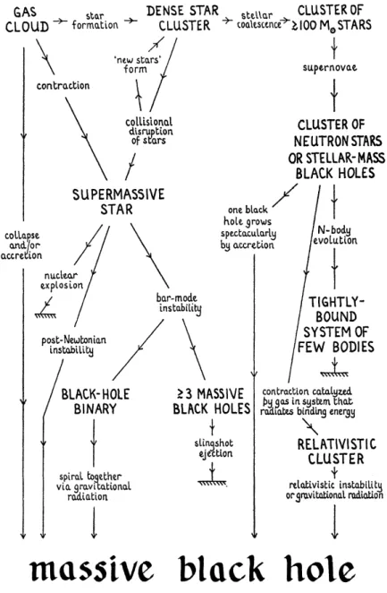
Gravitational collapse is one of the major processes considered in the formation of super-massive black holes (M & 106 Mo). These objects are believed to lie in the centres of the majority of galaxies, if not all. The most convincing argument has certainly been raised by Rees (1978) with his famous flow chart, reproduced in Fig. 5. The aim of this flow chart is to show that, given the high luminosity of AGN, a large amount of material must have been involved in their formation and “the almost inevitable endpoint [...] [is] the collapse of a large fraction of its total mass to a black hole” (Rees 1984).
It was realized at the end of the ’70s that gravitational energy could be quite efficiently converted around black holes. Considering the accretion by a non-rotating black hole, the binding energy of the last circular orbit for a test particle of mass m is √38mc2, a process extracting the remaining energy would have an efficiency of 1−√8
3 =
5.7%. For a maximally rotating black hole, the efficiency of conversion of the energy of the accreted matter energy goes up to 42%, sixty times larger than for hydrogen fusion. Blandford & Payne (1982) proposed a mechanism tapping this energy reservoir based on the magnetic field anchored in the disk, which can generate a magneto-hydrodynamic 4Even assuming that the observed variations come from a boosted region of Doppler factor δ, the gravitational energy can not be neglected unless δ À 30.
5The Schwarzschild radius R
S of a system of mass M is simply defined as the size for which the escape velocity equals the speed of light, vesc= c. For a test mass m with the simple classical argument1
2mv 2
Figure 5. Possible modes of formation of a super-massive black hole in an AGN. Extracted from Rees (1978).
wind along the rotation axis (Ferrari 1998). The power extracted from the accreted material would then be:
(1.7) LBP∼ Bd2R2disk r GM Rdisk ∼ 2 × 10 46 µ Bd 103G M 109M o ¶2 erg s−1 where the inner radius of the accretion disk is assumed to be Rdisk ∼ 5RS. Using Eq.(5.6) in Blandford & Payne (1982), the typical efficiency of the process is on the order of 12%.
One can compare this power to the Eddington luminosityLE, which is the maximal steady state luminosity of a spherical system powered by accretion. One assumes that the gravitational force exerted on electron-proton pairs in a fully ionized plasma is balanced by the radiation pressure of an inner shining object when the luminosity attains the critical valueLE. The radiation pressure mostly acts on the electrons, and is accounted for using the Thomson cross section σT, while the gravitational force mostly acts on the protons of mass mp ∼ 1800me and one assumes that the plasma remains locally neutral so that charges are not separated. The Eddington luminosity is then:
(1.8) LE = 2πmpc3 σT RS∼ 1.26 × 1047 µ M 109M o ¶ erg s−1
The power could also in principle be extracted from the black hole itself. The energy of a rotating black hole (Kerr 1963) of mass M has indeed two components: one due to its spin and an “irreducible” mass that goes down M/√2 for a maximal rotation. The rotation energy could be extracted by slowing down the black hole and the efficiency of such a process would be Espin/Etot = (M c2− Mc2/
√
2)/M c2 ∼ 29%. Nonetheless, it is not easy to build a realistic astrophysical scenario able to extract all of this energy. Blandford & Znajek (1977) proposed a scenario where the black hole is seen has a resistive sphere (though with a small surface resistivity on the order of∼ 100 Ω). In an ambient magnetic field B0, power can be extracted using a current flow between the equator and the poles, with a maximum value of:
(1.9) LBZ∼ B02 µ J Jmax ¶2 µ RS 2 ¶2 c∼ 3×1046 µ B0 104G M 109M o J 0.5Jmax ¶2 erg s−1
In this equation B0 is the magnetic field close to the black hole, which is assumed here to be ten times larger6 than the magnetic field at Rdisk, which is used in Eq. (1.7). By slowing down the black hole from a maximal spin J = Jmax to J = 0, a fraction of 9.2% of the rest energy can be extracted (Rees 1984). This scenario is based on a strong magnetic field and the most natural explanation for its origin would be the accretion disk that feeds the black hole with matter and “frozen-in” magnetic lines.
The mechanisms of Blandford & Znajek (1977) and Blandford & Payne (1982) do not exceed the limiting Eddington luminosity and both generate jetted outflows that are sufficiently powerful to explain the giant structures observed in radio or the emission at higher energies. They provide a direct link between the black hole and the jet or between the accretion disk and the jet, where rotating magnetic fields are a crucial ingredient, but distinctive signatures of these mechanisms are not yet clearly identified. A recent review of the various processes at play in the ejection and collimation of jets as well as the tremendous efforts of simulations and observations ongoing on this topic can be found in Pudritz et al. (2012).
1.1.2.3. The geometric unification scheme
AGN are thought to host a black hole, which is fed by an accretion disk. As discussed in Sect. 1.1.1.3, AGN are usually divided in radio-loud and radio-quiet objects, the latter not exhibiting jets. Both sub-classes can exhibit emission lines, believed to emerge from the photo-ionization of a small region of dense, fast moving clouds (the broad line region, BLR) and of a larger zone with slower moving clouds (the narrow line region, NLR).
NLRGs and radio-quiet Seyfert 2 do not exhibit broad lines. Rowan-Robinson (1977) assumed that, instead of being absent, BLR are hid-den, or obscured by dust. Observing the polarized light from the Seyfert 2 prototype NGC 1068, Antonucci & Miller (1985) found a spectrum very similar to a Seyfert 1. This is understood as light being scattered and polarized by electrons in the material above the nucleus (see e.g. the review of Shields 1999) and it confirms the “hidden” BLR hypothesis. An extra ingredient in the AGN unification scheme was 6The solutions studied by Blandford & Payne (1982) correspond to a self similar magnetic field B ∝ R−5/4.
added: a dusty torus or a wrapped disk obscuring the light of type 2 objects.
The unification scheme that has emerged combining these ingredi-ents (black hole, disk, jet, torus and clouds) is usually attributed to Antonucci (1993) and Urry & Padovani (1995). As shown in Fig. 6, it is based on orientation effects compared to the line of sight.
Figure 6. Unification scheme of AGN. The acronyms for the different sub-classes of AGN are given in Fig. 2. Adapted from Urry & Padovani (1995) .
1.2. Jetted emission of blazars 1.2.1. Transferring the jet energy to particles
The mechanisms launching the jet and the processes converting the jet energy into particle kinetic energy are thought to be related to the matter content of the jet. It is widely accepted that at least half of the electromagnetic spectrum of AGN is radiated by electrons, but for the plasma to remain neutral, they must have a positive counterpart: positrons (in which case one speaks of pair plasma) or ions/protons (referred to as protons or normal matter in the following).
1.2.1.1. The jet content
The matter content of the jet is usually thought to be linked to the mechanism responsible for the launch of the jet. Processes tapping the black hole rotational energy (e.g. Blandford-Znajek) are often assumed to yield pair plasma jets while the content of outflows originating from rotating disks (e.g. Blandford-Payne) is assumed to be extracted from the disk itself and should therefore be an electron-proton plasma.
But the variety of astrophysical scenarios is far more complex. As discussed before, the magnetic field embedding the black hole may be partly fed from the disk, conveying normal matter together with the lines (McKinney & Gammie 2004; De Villiers et al. 2005). The opposite can also happen if a very small amount of matter is loaded on the magnetic field lines anchored in the disk. In this case, the interaction of the disk emission with the magnetic field could produce a pair plasma (a possibility that has not been yet deeply investigated according to Spruit 2010).
Whatever the power source, either black hole rotation or accretion, and whatever one jet contains, either pair plasma or normal matter, an efficient process must convert the energy at the base of the jet into particle kinetic energy. Depending on the author, the energy at the base of the jet is referred to as “centrifugal” or “magnetic” and the use of “Poynting flux” is widespread. Spruit (2010) argues that these quan-tities are in general equivalent. If one considers the frame co-rotating with the power source, then the matter flow is parallel to the magnetic field lines and the Lorentz force ∝ v × B is null - only the centrifugal force drives the flow. In an inertial frame there is no centrifugal force but it is the azimuthal component of the magnetic field that drives the flow, hence the magnetic energy denomination. These two equivalent
forces can be seen as participating in the conversion of electromagnetic energy into kinetic energy. Indeed, in magneto hydrodynamics, as in simple vacuum electrodynamics, E = v× B, and the Poynting flux reads, in cgs:
(1.10) Π = c
4πE× B = v⊥ B2 4π
where v⊥ is the component of the flow velocity that is orthogonal to the magnetic field. Eq. (1.10) shows that the Poynting flux in magneto hydrodynamics is the flux of magnetic energy advected with the fluid in a direction orthogonal to the magnetic field. Spruit (2010) observes that the Poynting flux plays a role similar to a flux of enthalpy in regular hydrodynamics. In analogy with Bernoulli’s theorem, the sum of the enthalpy (∝ B2) and kinetic energy of the fluid (∝ v2) is conserved. The increasing particle energy along the jet is progressively extracted from the magnetic field.
The fraction of the magnetic energy going into kinetic energy is model dependent. Standard scenarios assume that the jet is axisym-metric (rotational symmetry around the jet axis) and the maximum bulk Lorentz factor achieved is Γ∞ ∼ σ1/3, where σ is the ratio of the magnetic and kinetic energy at the base of the jet (calling B0 and ρ0 the magnetic field and the particle density at the base of the jet, σ = B02
8π/12ρ0c2). If all the energy was converted, by definition of σ, one would get Γmax = σ. Defining the efficiency η of the process as the ratio between the achieved particle energy and the maximal one, one gets (1.11) η = Γ∞ρc 2 Γmaxρc2 ∼ σ −2/3= 1 Γ2 ∞
The conversion of Poynting flux to the flow of particles is then effi-cient for mildly relativistic flows and ineffieffi-cient for high velocity flows. This conclusion is drawn for axisymmetric, i.e. 2D flows. 3D modelling of the system including kinking modes/reconnection (cf. next subsec-tion) can be much more efficient, with values of up to 50% for Lorentz factors of∼ 20, being reached after a distance from the base of the jet of 102− 103 R
S (Giannios & Spruit 2006; Komissarov et al. 2007). Despite the high efficiency of the above-mentioned magnetic dissi-pation processes (see also Blandford 2002), the acceleration of particles
remains mostly attributed to shocks (Blandford & Rees 1974; Begel-man et al. 1984), the efficiency of which is still a matter of debate. The simulations of the latter tend to produce broad distributions of particle Lorentz factors while the former are still limited (potentially by numerical constraints).
To support the large energetics of giant radio lobes, there should be a fraction of protons in the jet. Sikora et al. (2005) argue that a scenario involving shocks favours such a proton domination of the energy flux. Authors, such as Marscher (2006), suggest an intermediate picture where reconnection-like scenarios, which are more likely linked to pairs and can be much more efficient, would occur in an initial phase and feed the shocks with already energized particles. The interested reader can also refer to the theoretical work of Petrosian (2012) and the simulations of Sironi & Spitkovsky (2009) where turbulence acts as the injector of particles in the shock.
1.2.1.2. Acceleration processes
An acceleration process extracts energy from the medium and feeds it to the particles. This can be done through a scattering of the particles off irregularities in the magnetic fields or simply through reflections on “magnetic walls”. The generic equation to study the evolution over time t of a distribution of particles’ energy, or equivalently of a Lorentz factor distribution N (γ), is the Fokker-Planck equation:
(1.12) ∂N ∂t (γ, t) + ∂ ∂γ [ ˙γN (γ, t)] = Q(γ, t)− N (γ, t) tesc
where the diffusion term is neglected. In Eq. (1.12), Q(γ, t) is the source term, tesc is the time needed for the particle to escape the region and ˙γ is the energy loss/gain term. The latter includes the acceleration of particles (positive contribution), characterized by a time scale tacc, as well as the various radiative losses (negative contributions) that I dis-cuss in Sect. 1.2.2.17. I assume here for the sake of simplicity that the loss processes are slow compared to the acceleration ones, so that there is only one contribution to the loss/gain term: ˙γ = γ/tacc. Assum-ing that no source injects particles when the steady state is reached, Eq. (1.12) reads, after a development of the derivative of the loss/gain 7For the sake of clarity, the acceleration and escape times are assumed inde-pendent of γ, but an integral solution can be derived in a more general context
term: (1.13) γdN (γ) dγ =−N(γ) × µ 1 +tacc tesc 
which is solved for a particle spectrum N (γ) ∝ 1/γ1+tacc/tesc, i.e. a
power law of index 1 + tacc/tesc. A process that accelerates particles at high energies (hard spectrum, i.e. small index) is thus a process for which the ratio tacc/tesc is as small as possible, i.e. a process that has a fast acceleration rate.
In the late ’40s, Enrico Fermi designed a mechanism which stochas-ticly accelerates charged particles through collisions with magnetized clouds of randomly oriented velocity U (Fermi 1949). Following Begel-man et al. (1984), for a relativistic particle of speed c, each bounce yields an energy change|∆γ/γ| ∝ U/c with an increase when the col-lision is head on and a decrease when the cloud is moving away. The head-on collisions are more frequent and the energy increase is favoured by an amount U/c, so that the acceleration time is ta∝ (c/U)2. Since the clouds are slower than the speed of light c/U < 1, this quadratic process (called the second order Fermi process) is quite slow. He then designed in the beginning of the ’50s (Fermi 1954), a first order process with ta ∝ c/U, where only head-on collisions occur in a “contracting magnetic bottle” (Petrosian 2012). The latter is faster and thus much more efficient.
Acceleration by shocks can be as efficient as a first-order Fermi pro-cess, in which case authors speak of diffusive shock acceleration (see e.g. Drury 1983), or as a second-order Fermi process, called stochastic shock acceleration (see e.g. Petrosian 2012, for a recent approach). Not until recently has magnetic reconnection been recognized as a first or-der Fermi process, as discussed in the following. Both mechanisms are triggered by an initial disturbance in the medium. If the disturbance travels faster than the speed of sound, a shock is formed and the par-ticles are accelerated as they cross the front. In a highly-magnetized plasma, the magnetic field lines are anchored with - “frozen in” - the matter and they become tangled as the flow advects them. If the re-sistivity of the plasma is not null, Joule dissipation locally causes a heating of the matter which conveys magnetic lines. Reconnection of opposite direction lines thus occurs, which can efficiently accelerate particles.
Figure 7. Schematic view of shock acceleration (left) and magnetic reconnection acceleration (right) in panels a). Panels b) show the reflections of the particle on inhomogeneities or on the magnetic “walls” with the dashed line. Panels c) show simplified views as box models. Adapted from Drury et al. (1999); Drury (2012).
I show in Fig. 7 a schematic view of the two acceleration processes. In the following, I adapt the “box model” approach and derive the acceleration and escape times in these two scenarios. A more detailed discussion and a more rigorous approach can be found in Drury et al. (1999); Drury (2012) and references therein. The escape rates are in both cases determined by the speed of the outflow and the typical scale involved (l for shocks, L for reconnection). The flow leaves the box from two sides for reconnection, hence the factor of 2 in the velocity (first line of Table 2).
The acceleration rate corresponds to the velocity change on each side of the box. Since only one direction of motion is accounted for and since the particles’ motion is assumed to be isotropic, only a third of the particles are effectively accelerated at this rate (the same classic
Shock acceleration Magnetic reconnection
Escape rate tesc1 = U2
l tesc1 = 2U2 L Acceleration rate t1 acc = 1 3|U 1−U2| l tacc1 = 1 3|2Ul1 −2UL2| Ratio tacc tesc = 3 |U1U2−1| tacc tesc = 3 |U1LU2l−1| Mass flux conservation ρ1U1A = ρ2U2A 2ρ1U1A1 = 2ρ2U2A2 Power law index 1 +tacc
tesc = 1 +
3
|r−1| 1 +ttaccesc = 1 +
3 |r−1| Table 2. Derivation of the index of the power-law dis-tribution of the accelerated particles for the “box mod-els” of the shock acceleration (second column) and mag-netic reconnection (third column). In both cases the compression ratio is defined as r = ρ2/ρ1.
argument as in the kinetic theory of gases). One can then simply compute the ratio of these rates and combine it with the conservation of mass flux, as in the third and fourth lines of Table 2, to obtain the index of the electron power law. The compression ratio r = ρ2/ρ1 is particularly useful, and in both cases:
(1.14) N (γ)∝ 1/γ1+|r−1|3
The compression ratio can be derived precisely in the case of a strong shock, for a perfect gas. Using the conservation of energy flux, the conservation of momentum flux and assuming a mono-atomic gas one gets r = 4, which yields a power law of index 2 for shocks. The case of magnetic reconnection is less constrained. Indeed the conservation of momentum flux is trivial since the total input and output momenta are null. With the sole constraint of the conservation of energy flux, one cannot derive r. Drury (2012) argues that, for reconnections, one expects a much denser output medium than the input one, yielding rÀ 1 and an index tending towards 1.
These very simple derivations of indices are in good agreement with particle-in-cells simulations, e.g. Zenitani & Hoshino (2001); Drake et al. (2006) for magnetic reconnection and Sironi & Spitkovsky (2009) for shock acceleration. In this simple approach, the energy dependency of the time scales is not explicitly taken into account and the maximum energy to which particles can be accelerated is determined by the escape time8, presumably decreasing with energy, and by the radiative losses, which are discussed in the following.
1.2.2. Radiation of the accelerated particles 1.2.2.1. From particles to photons
The processes that convert the energy of a particle into γ rays can be divided into two sub-classes: the matter-matter interactions and the matter-field interactions.
γ rays produced by matter-matter interactions in astrophysical en-vironments could come from hadronic processes, mostly from photo production of pions, i.e. interactions of protons with ambient pho-tons (from the jet itself or from its environment in the case of AGN): p + γ → p + π0. π0 have a life time of ∼ 10−16 s and decay, with a branching ratio of 99%, into two γ rays of ∼ 135 MeV/2 = 67.5 MeV in the particle rest frame. After integration over the pitch angle and af-ter Lorentz transformation, the γ-ray spectrum produced by hadronic interactions is almost identical to that of the parent population at the highest energies, i.e. above the bulk emission around 67.5 MeV that constitutes a smoking gun of these interactions. Another smoking gun would be the detection on Earth of neutrinos of astrophysical origin from an equivalent channel such as p + γ→ n + π+. Indeed a charged pion decays with probab 99.99% into a muon and the associated trino and the muon itself decays into an electron and associated neu-trinos: π+→ νµ+ µ+→ νµ+ ¯νµ+ νe+ e+.
The production of γ rays can also originate from matter-antimatter annihilation. The first channel to consider is the annihilation of positrons with electrons producing, in the centre-of-mass frame, two γ rays emit-ted back-to-back with energies mec2 = 511 keV. This emission line, broadened by relative motion, tracks the areas where the density of matter is large, such as the galactic plane, and can, for instance, be 8Note that the size of the magnetic reconnection region is a priori smaller than that of a shock, which should yield a smaller maximum energy.
studied with the INTEGRAL satellite (see e.g. Kn¨odlseder et al. 2005). The counterpart of this annihilation process is pair creation by two photons, which is responsible for the absorption of γ rays during their propagation, discussed in Sect. 1.3.2. Besides the annihilation of elec-trons, any particle-antiparticle pair can produce γ rays, each of them carrying half of the total energy in the centre-of-mass frame. Such annihilations can be exploited in the search for dark matter, which represents 23% of the energy content of the Universe. Weakly inter-acting massive particles (WIMPs) are one of the leading dark matter particle candidates and they could annihilate producing lines between 10 GeV and a few TeV (Drees & Gerbier 2012). An apparent excess around∼ 130 GeV (e.g. Su & Finkbeiner 2012; Weniger 2012) near the Galactic centre has recently triggered some excitement but has not yet been confirmed by the Fermi-LAT collaboration and could still be of systematic origin.
When considering the interaction of matter with an electromagnetic field, or equivalently with a photon, one must account for synchrotron losses for a magnetic field, Compton scattering for a collision with a photon and bremsstrahlung when the Coulomb field of a nucleus is involved. The latter, combined with pair creation in the field of a nu-cleus, explains the development of atmospheric showers, discussed in Sect. 1.3.1.1. Synchrotron emission of electrons is the most favoured process to explain the emission of AGN from radio to X rays. It has also been invoked for proton emission at higher energy (Aharonian 2000). Depending on the modelling (M¨ucke & Protheroe 2001), this process could even dominate over photo production of pions, elimi-nating the neutrino smoking gun for proton acceleration (but see also Cerruti et al. 2012, for a mixed model). The synchrotron emission has a counterpart, synchrotron self absorption, which occurs when the brightness of a synchrotron source becomes high enough to heat up the emitting population. Below a critical frequency, the emitting re-gion becomes opaque to its own radiation or “optically thick” and the emitted spectrum follows a power law EdNdE ∝ E5/2.
The most favoured process to explain the γ-ray emission of AGN is Compton scattering. In its usual formulation, it consists of the “col-lision” of a photon with an electron in a frame where the electron is at rest. The final state consists of a photon that has lost a fraction of its energy and an electron with a recoil energy. If the incoming
photon energy is negligible compared to the mass of the electron, the collision is almost elastic and the scattering occurs in the so-called Thomson regime where no direction is preferred. At higher photon energy, in the so-called Klein-Nishina regime, the recoil of the electron becomes non negligible, the angular distribution of the outgoing parti-cles is increasingly front sided and the interaction cross section drops. In astrophysics, one usually considers the frame where an energetic electron transfers its energy to a low-energy photon and the process is called inverse Compton. If the electron has a Lorentz factor γ and the photon has an energy hν in the observer frame, then the photon has an energy ∼ γhν in the electron frame. In the Thomson regime γhν ¿ mec2, the outgoing photon energy remains γhν while in the Klein-Nishina regime, the electron transfers almost all of its energy to the photon γhν = mec2. Back in the observer frame, the outgoing photon has then an energy γ2hν in the Thomson regime and an energy γmec2 in the Klein-Nishina limit. A natural origin of the Comptonized photon field is the synchrotron radiation of the electrons, in which case the emission scenario is called synchrotron self Compton (see Band & Grindlay 1985), which I discuss in the next subsection. When the pho-ton field does not come primarily from the electrons themselves, one speaks of external Compton. Though presumably less important in BL Lacs and potentially dominant in FSRQs, external photon fields, e.g. from the BLR or from the accretion disk (see e.g. Dermer & Schlickeiser 1993; Sikora et al. 1994), can also be scattered by the electrons.
1.2.2.2. The synchrotron self Compton model
I consider an electron of energy γmec2, moving at an angle θ with respect to the magnetic field of norm B. The particle loses energy via synchrotron processes and emits radiation at the frequency ν, or equivalently emits photons of energy hν. The synchrotron energy losses per frequency band and per unit solid angle for a Lorentz factor γ are defined as: dPsync dΩ (ν, γ, θ) = d dΩdν¡−mec 2˙γ sync¢ = d dΩdν µ −dE dt sync ¶ = 2σTcγ2× UB× f(ν) sin2θ 2π (1.15)
where UB = B2/8π is the magnetic energy density (in cgs) and σT = 8π 3 h e2 mec2 i2
is the Thomson cross section. I normalize the function f (ν) to unity so thatR∞ 0 f (ν)dν = 1 and: (1.16) f (ν) = 9 √ 3 8π 1 νC Fµ ν νC 
where the critical angular frequency is defined with 2πνC = 32meBecγ2sin θ. The function F is linked to the modified Bessel function K5/3 via F (x) = xR∞
x K5/3(t)dt and can be found in the GNU scientific library, for computational purposes. Assuming that the magnetic field is tan-gled with matter and that the emission of the synchrotron radiation is isotropic in the emitting region frame (sometimes called a “blob”), the total synchrotron energy losses are:
(1.17) Psync(ν, γ) = Z dΩdPsync dΩ (ν, γ, θ) = 4 3σTcγ 2× U B× f(ν) The other losses that I consider here come from the interaction of the electron with a field of photons through inverse Compton. Assum-ing an isotropic field of photons of energies hν0 = ²0mec2and averaging over the arrival direction of the electron:
(1.18) PIC(ν, γ) = 4 3σTcγ 2× m ec2 Z d²0n(²0)²0× g(ν, γ, ν0) where n(²0) is the density of photons per energy band, so that nph = R d²0n(²0) is the number of photons per unit volume and that the quantity Uph = mec2R d²0n(²0)²0 is the photon energy density. Like f (ν) for the synchrotron radiation, I normalize g(ν, γ, ν0) to unity, i.e. R∞
0 dνg(ν, γ, ν0) = 1. I simply define this function as g(ν, γ, ν0) = 6x2(1− x)/ν, with x = ν/ν0
4γ2 ∈ [0; 1], in the Thomson scattering limit
and for an ultra-relativistic electron (derived from Eq.(7.26b) in Ry-bicki & Lightman 1979). To account for the reduction of the cross section for non-facing collisions derived by Klein and Nishina, Jones (1968) computed an approximated expression that reads (with my def-inition of g and a bit of algebra):
(1.19) g(ν, γ, ν0) = 9x 2
ν [2κ ln κ + (1− κ) × (1 + 2κ + γ²0x)] where κ−1= x−1− 1 and κ ≥ 1/4γ2 for kinematic reasons.
Eq. (1.18) and Eq. (1.17) are remarkably similar. After integration over the frequency (f and g are normalized to unity), both losses are proportional to γ2B2 and the ratio of the total inverse Compton over synchrotron losses for a single particle is simply the ratio of the photon field over magnetic field energies Uph/UB.
Instead of a single electron, I now deal with a distribution, say e.g. a power law ne(γ)∝ γ−p, where ne is the number of electrons per unit volume. The spectral luminosity, in energy per unit time per frequency band, is derived by integrating over the volume of emission and over the electron distribution. For a spherical homogeneous emission region of radius R, assuming that its light crossing time is small with respect to the radiative time scales:
(1.20) Lsync(ν) = 4π 3 R 3×3 2 1−τ22 [1− e−τ(1 + τ )] τ Z dγne(γ)Psync(ν, γ) where the middle expression characterizes the synchrotron self absorp-tion and tends to one for a null optical depth. Using Gould (1979), the latter reads: (1.21) τ (ν) = 1 4π R× (c/ν)2 mec2 Z dγ ½ −γ2 d dγ · ne(γ) γ2 ¸¾ Psync(ν, γ) In the SSC model, the field of photons which is “Comptonized” by the electrons is the very field that they create through synchrotron losses. Since n(²0) varies in the emission region (Gould 1979), an av-erage corrective factor αcorr = 3/4 is applied (as in Kataoka 1999; Sanchez 2010), so that the photon field energy density and the syn-chrotron power are linked with:
(1.22) mec2n(²0)²0d²0 = αcorrR c × 1− eτ (ν0)2 τ (ν0) 2 × ·Z dγ′ne(γ′)Psync(ν0, γ′) ¸ dν0 The inverse Compton luminosity then reads:
LIC(ν) = 4 3πR 3×3 2 1−τ22 ee[1− e −τee(1 + τ ee)] τee × σT R Z dγne(γ)γ2 Z dν0 1− e−τ (ν0)2 τ (ν0) 2 g(ν, γ, ν0) Z dγ′ne(γ′)Psync(ν0, γ′) (1.23)
where the absorption factor takes into account the pair creation. Fol-lowing Coppi & Blandford (1990), the associated optical depth is well approximated by:
(1.24) τee(ν) = 0.2σTR× nµ me c2 hν
The observed flux F (νobs) (in energy per unit time per unit area per frequency band) accounts for the luminosity distance of the source DL, F (νobs) = Lobs(νobs)/4πDL2, and also for its redshift, dividing the frequency by 1 + z. The Doppler effect increases the frequency by a factor δ, νobs = δν/(1 + z), and enhances the flux normalization by a factor δ3, as in Sect. 1.1.2.19. The observed flux is, therefore:
(1.25) F (νobs) = δ3 1 4πD2L × Ltot µ (1 + z)νobs δ ¶ × e−τEBL(hνobs)
where Ltot = Lsync + LIC is the total SSC luminosity. The last term quantifies the transparency of the Universe to γ rays, discussed in Sect. 1.3.2.
1.2.2.3. The delta approximations and equipartition I discuss in the following the SSC modelling by imposing null opac-ities τ (ν) = τee(ν) = 0 and exploiting delta approximations. The first delta approximation is very common and is based on the fact that the function F (x) in Eq. (1.16) is maximum for x = 0.29. With my appro-priate normalization of f (ν), I thus assume that f (ν) = δ(ν− γ2νB), where δ is the Dirac function and νB = 0.29νC/γ2 ∝ B. Then from Eq. (1.17) and Eq. (1.20), the synchrotron luminosity Lδ
syncin the delta approximation reads: Lδsync(ν) = 4π 3 R 3×4 3σTc× UB× Z dγne(γ)γ2δ(ν− γ2νB) = 4π 3 R 3×4 3σTc× UB× Z dγne(γ)γ2δ(γ−pν/νB)× 1 2γνB = 4π 3 R 3×4 3σTc× UB 2νB × r ν νB neµr ν νB ¶ (1.26)
9I assume here that the angular size of the emitting region is smaller than the inverse of the jet Lorentz factor.
where the transition from the first to the second line exploits the transformation of the Dirac function under a change of variable, i.e. δ(x)dx = δ(h(x))h′(x)dx.
I can apply the same procedure to the inverse Compton, assuming a Dirac distribution for the function g (this is a less common delta approximation which I use for the sake of clarity and ease of com-prehension). Localizing analytically the maximum of g with its full expression in the Klein-Nishina regime is not straightforward and I use its simple expression in the Thomson regime, which peaks at 2γ2ν
0, so that g(ν, γ, ν0) = δ(ν − 2γ2ν0). Using Eq. (1.17) and Eq. (1.23), the inverse Compton luminosity in the delta approximation and assuming null optical depths is then:
LδIC(ν) = 4π 3 R 3× σ TR× 4 3σTc× UB× Z dγne(γ)γ2 Z dν0δ(2γ2ν0− ν)× Z dγ′ne(γ′)γ′2δ(γ′2νB− ν0) = 4π 3 R 3× σ TR× 4 3σTc× UB 4νB × Z dγne(γ) r ν 2γ2ν B ne µr ν 2γ2ν B ¶ = σTR 2 Z dγne(γ)Lδsync µ ν 2γ2 ¶ (1.27)
I show in Eq. (1.27) that assuming an electron distribution func-tion (EDF) peaking at ¯γ, ne(γ) = ne,0δ(γ− ¯γ), the inverse Compton luminosity is simply the synchrotron luminosity, scaled up by a factor ne,0σTR/2, and shifted to frequencies 2¯γ2 times larger.
As shown in Sect. 1.2.1.2, a power-law EDF is expected from accel-eration processes, which reads ne(γ) = ne,0γ−p for γ∈ [1; γmax]. Then from Eq. (1.26): Lδsync(ν) = 4π 3 R 3×4 3σTc× UB 2νB × ne,0× µ ν νB ¶−p−12 for ν ∈ [νB; γmax2 νB] ∝ ne,0× R3× B p+1 2 × ν− p−1 2 (1.28)