A numerical approach to variational problems
subject to convexity constraint
G. Carlier
∗, T. Lachand-Robert
†, B. Maury
†November 24, 1999
Abstract
We describe an algorithm to approximate the minimizer of an ellip-tic functional in the formRΩj(x, u, ∇u) on the set C of convex func-tions u in an appropriate functional space X. Such problems arise for instance in mathematical economics [4]. A special case gives the convex envelope u∗∗0 of a given function u0.
Let (Tn) be any quasiuniform sequence of meshes whose diameter
goes to zero, and In the corresponding affine interpolation operators.
We prove that the minimizer over C is the limit of the sequence (un),
where un minimizes the functional over In(C).
We give an implementable characterization of In(C). Then the
finite dimensional problem turns out to be a minimization problem with linear constraints.
1
Introduction
Let Ω be some bounded open convex subset ofR2, and
C := {u : Ω → R ; u is convex in Ω} .
We consider the variational problem subject to convexity constraint:
inf
u∈C∩KJ(u) with J(u) =
Z
Ωj(x, u(x), ∇u(x)) dx
(1)
∗Universite´ Paris IX Dauphine, Ceremade, [email protected].
†Universite´ Pierre et Marie Curie, Laboratoire d’Analyse Nume´ rique, 75252 Paris Cedex 05, France.
where K is a closed convex subset of a given space X = H1(Ω) or X = L2(Ω),
and j is a quadratic function of u and ∇u. We assume that C ∩ K is non-empty. If J is lower semicontinuous coercive and strictly convex on K, then existence and uniqueness of a minimizer of (1) directly follows from standard arguments. Throughout this paper, we shall always assume that J is such a functional.
A first example of such a functional is
Jf(u) = Z Ω · 1 2|∇u(x)| 2 + f (x)u(x) ¸ dx (2)
with f ∈ L2(Ω) given. Consider J = Jf, and K = X = H01(Ω), then (1)
is a classical projection problem in H1
0. Indeed it is equivalent to find the
projection of uf = ∆(−1)f onto C (the resolvent of the Laplace operator is
intended in H1
0, that is, with homogeneous Dirichlet boundary conditions),
as one can see from the identity
2Jf(u) = k∇(u − uf)k2L2(Ω)− k∇ufk2L2(Ω).
We can generalize to f ∈ H−1(Ω), writing hf, ui instead ofR f (x)u(x) dx. Another example is X = L2(Ω),
Ju0(u) = ku − u0k
2
L2(Ω) (3)
where u0 ∈ L2(Ω) is given, and
Ku0 = {u ∈ L
2
(Ω) ; u ≤ u0 a.e.} (4)
Then the solution of (1) with J = Ju0 and K = Ku0 is the convex envelope u∗∗0
of u0, that is the largest convex function in Ku0 [3], [5].
We will prove in Section 4 that the solutions of these two problems with u0 ∈ H01(Ω) and f = ∆u0 are, in general, different.
The aim of this paper is to give a numerical scheme to approximate so-lutions of (1).
1.1
Notations
In all the following we will use classical notations and assumptions from numerical analysis. Let (Tn)n∈N be a sequence of quasiuniform regular
trian-gulations of the domain Ω, Mn
i = (xni, yin) ∈ Ω, i = 1, . . . , kn, are the nodes
of Tn, and hn is the largest edge length of all triangles in Tn. We assume
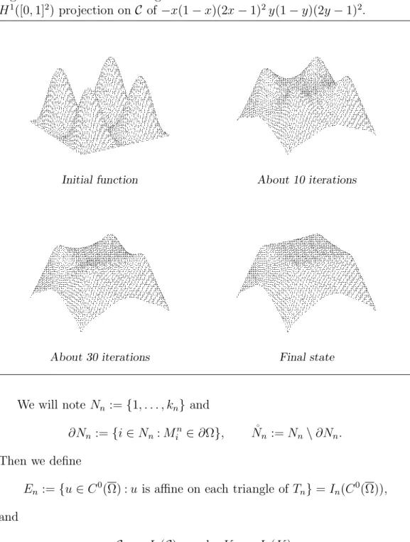
Figure 1: Iterations of the algorithm.
H1([0, 1]2) projection on C of −x(1 − x)(2x − 1)2y(1 − y)(2y − 1)2.
Initial function About 10 iterations
About 30 iterations Final state
We will note Nn := {1, . . . , kn} and
∂Nn := {i ∈ Nn: Min∈ ∂Ω}, N˚n:= Nn\ ∂Nn.
Then we define
En := {u ∈ C0(Ω) : u is affine on each triangle of Tn} = In(C0(Ω)),
and
Cn:= In(C) and Kn:= In(K),
where In is the affine Lagrange interpolate operator from C0(Ω) to En. One
can easily show that Cn is a finite dimensional closed convex cone with
1.2
Approach
Our basic idea is to approximate problem (1) by: min
u∈Cn∩Kn
J(u) (5)
and let n go to infinity.
This scheme is therefore based on external approximations of the cone of convex functions. As noted by P. Chone´ [2], there is very little hope that methods where C is internally approximated by C ∩Enshould converge to the
solution of (1). Indeed the affine Lagrange interpolate of a convex function need not be convex and the cone Cn is in some sense much bigger than C ∩En.
This somehow surprising fact is enlighted by the following example: consider Ω = (0, 1)2, with a mesh consisting of two triangles having their common
edge in {x1 = x2}. The function u(x1, x2) = (x1+ x2)2 is convex whereas its
interpolate is a concave function.
More precisely, we have the proposition:
Proposition 1 Assume that there are 2 directions h and k such that: (ν · h).(ν · k) ≥ 0
for every vector ν which is normal to an edge of every triangle of the trian-gulation Tn, for all n. Then if u is the limit in L∞loc of a sequence (un), with
un ∈ C ∩ En for all n, we have:
∂2u
∂h ∂k ≥ 0 (6)
in the sense of Radon measures.
For instance, in a structured mesh of the form , the normal vectors are v1 = (1, 0), ν2 = (0, 1) and ν3 = (1, −1). Hence, we can choose h = (1, 0),
k = (0, −1), and get
u = lim un in L∞loc, with un∈ C ∩ En =⇒
∂2u
∂x ∂y ≤ 0
in the sense of measures. This inequality obviously does not hold for all convex functions.
As a consequence, it appears that convex functions that do not satisfy the constraints (6) cannot be approximated (even in the sense of distributions) by convex functions of En. This is the very reason for which we chose an
Proof. This result is proved in [2] but we recall it here for sake of com-pleteness. Let u be in En, then u ∈ C if and only if, for every pair of adjacent
triangles 1 and 2 of Tn, we have:
(q2− q1) · ν12≥ 0,
where qi is the value of ∇u in triangle i = 1, 2, and ν12 is the normal unit
vector pointing from 1 to 2.
Assume now that h and k satisfy the assumption of the previous propo-sition and let ϕ be some nonnegative smooth function with compact support in Ω. Summing up Green’s Formula in every triangle of Tn yields:
¿ ∂2u ∂h∂k, ϕ À = − X T ∈Tn ¿ ∂u ∂h, ∂ϕ ∂k À =X e ((q2 − q1) · ν12)(ν12· h)(ν12· k) Z eϕ(s)ds ≥ 0
where the last summation is taken over all interior edges e of Tn.
A similar proposition can be given as a pointwise property:
Proposition 2 Let u ∈ C2(Ω) be a convex function which is limit, in C0(Ω),
of a sequence (un) ⊂ C ∩ En.
Let (Mn
in) be a convergent sequence of nodes of the triangulations, with
limit M ∈ Ω. Let, for all n, Mn
jn be a node adjacent to (M
n
in), and ν a cluster
point of the sequence Minn−Mjnn
|Mn in−Mjnn|
. Then
∂2u
∂ν ∂ν⊥(M ) ≥ 0
where ν⊥ is normal to ν and (ν, ν⊥) is direct.
Proof. Since un converges to u uniformly on any compact subset of Ω, and
all are convex functions, ∇un converges to ∇u a.e. in Ω.
The jump of ∇un on the edge [Minn, M
n
jn] is nonnegative by convexity;
passing to the limit for a subsequence, the property follows immediately.
2
Convergence
Let un (respectively u) denote the solution of (5) (respectively (1)). The
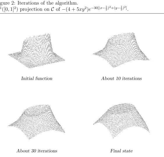
Figure 2: Iterations of the algorithm.
H1([0, 1]2) projection on C of −(4 + 5xy2)e−30[(x−21)2+(y−12)2].
Initial function About 10 iterations
About 30 iterations Final state
Theorem 1 The sequence (un) converges to u strongly in X and uniformly
on all compact subsets of Ω.
We will prove this theorem only in the case of the projection problem that is, J = Jf and K = X = H01(Ω). Other cases, with J strictly convex and
coercive, are similar. (In particular, the proof is even simpler for the gradient independent case since it does not require an estimate on the gradient.)
In order to prove this property, we first need the technical result: Lemma 1 There exists C > 0 such that, for all v ∈ W1,∞(Ω) ∩ C:
∀n ∈ N, k∇In(v)kL∞(Ω) ≤ C k∇vkL∞(Ω). (7)
and ∇In(v) → ∇v a.e. in Ω.
Step 1. Let T be an element of Tn, with vertices A, B, C. Writing e1 =
(B − A)/ |B − A|, we have
∇In(v) · e1 = v(B) − v(A)
|B − A| ≤ k∇vkL∞.
A similar relation holds for e2 := (C − A)/ |C − A|. Since the triangulations
are quasiuniform there exists C > 0 such that (7) is satisfied.
Step 2. Let D be the set of differentiability points of v which do not belong to any edge of the triangulations; D is clearly of full Lebesgue measure in Ω. For any M ∈ D, let ([An, Bn, Cn])n∈N be the sequence of triangles of Tn
containing M and whose vertices An, Bn, Cn converge to M . Define also the
unit vectors en1 := Bn− An |Bn− An| and en2 := Cn− An |Cn− An| .
Let pn, qn, rn be some subgradients of v respectively at An, Bn, Cn. By
mono-tonicity we have, for all n:
pn· en1 ≤ v(Bn) − v(An) |Bn− An| = ∇[In(v)](M ) · e n 1 ≤ qn· en1 pn· en2 ≤ v(Cn) − v(An) |Cn− An| = ∇[In(v)](M ) · e n 2 ≤ rn· en2.
Since v is differentiable at M , sequences pn, qn, rn all converge to ∇v(M)
(cf. [5]), and we get: ³
∇[In(v)](M ) − ∇v(M)
´
· eni −→ 0, i = 1, 2.
Since the triangulations are quasiuniform, it follows that ∇[In(v)(M )]
con-verges to ∇v(M).
This ends the proof of the lemma.
Proof of Theorem 1.
We recall that un is the projection of uf := ∆(−1)f onto Cn so that:
∀n ∈ N, k∇unkL2(Ω) ≤ k∇ufkL2(Ω) (8)
Since un is a minimizer in Cn, we have:
∀v ∈ C ∩ H1
Hence for all ε > 0, there exist vε ∈ W01,∞∩ C such that:
J (vε) ≤ J(u) + ε. (10)
From Lemma 1, there exists C > 0 such that:
k∇In(vε)kL∞ ≤ C k∇vεkL∞ and ∇In(vε) → ∇vε a.e.
Hence, by Lebesgue’s Dominated Convergence Theorem, we get: J(In(vε)) → J(vε).
Taking (9) and (10) into account, and since ε is arbitrary, we deduce: lim sup
n→∞
J (un) ≤ J(u). (11)
By (8), we may extract a subsequence, again labeled un and find some
u ∈ H1
0 such that un converges to u a.e. and strongly in L2(Ω) and ∇un
converges to ∇u weakly in L2(Ω).
We will prove that u is convex. By definition, for all n, un = In(vn), for
some vn∈ C. Let us fix now some convex set ω ⊂⊂ Ω.
Let us show first that (∇vn) is bounded in L∞(ω). If not, there would
exist xn ∈ ω such that, up to a subsequence, |∇vn(xn)| → +∞.
Up to subsequences, we may also assume that xn is converging and:
dn := ∇vn
(xn)
|∇vn(xn)| −→ d ∈ S 1.
Now, let x0 ∈ Ω be such that, for n large enough:
(x0− xn) · dn ≥
1
2|x0− xn|.
(Such a point exists since (xn) ⊂ ω ⊂⊂ Ω and dn converges.) Since vn is
convex, we get:
|∇vn(x0)| ≥
1
2|∇vn(xn)| −→ +∞.
Let en:= ∇vn(x0)/ |∇vn(x0)| and, extracting subsequences, assume that
it converges to e ∈ S1. Define Σ := ½ p ∈ S1: p · e ≥ 2 3 ¾ and Q := (x0+R+Σ) ∩ Ω.
If n is large enough, then for all p ∈ Σ, p · en≥ 12. Then, for any x ∈ Q (with
x = x0+ tp, t > 0, p ∈ Σ), the following holds:
|∇vn(x)| ≥ ∇vn(x) · p ≥ ∇vn(x0) · p ≥
1
2|∇vn(x0)| .
Since the rightmost member tends to infinity independently of x ∈ Q, it follows that k∇vnkL2(Q) → +∞. On the other hand, since the triangulations
are quasiuniform and vnis convex, this also implies k∇unkL2(Ω) → +∞ which
yields a contradiction with (8).
Hence, (∇vn) is bounded in L∞(ω). Standard interpolate estimate yields
that there exists a constant Cω such that:
kun− vnkL∞(ω)≤ Cωhnk∇vnkL∞(ω) −→ 0. (12)
This implies in particular that vn converges to u in L2(ω); hence u is convex
in ω. Since ω is arbitrary, u is convex in Ω.
From (11) and since u is convex, we deduce that u = u. Since (un) is
bounded in H1
0(Ω) and u is the only cluster point of (un) in the weak topology
of H1
0(Ω), we deduce that the whole sequence (un) converges weakly to u.
On the other hand, (11) yields:
k∇unkL2(Ω) −→ k∇ukL2(Ω)
and then (un) converges strongly to u.
It remains to show that un converges uniformly to u on compact subsets.
Let ω be any relatively compact open convex subset of Ω. We have kun− ukL∞(ω) ≤ kun− vnkL∞(ω)+ kvn− ukL∞(ω).
From (12), we just have to show that vn converges to u in L∞(ω). Since
we know that the sequence (vn) is uniformly Lipschitz, this is a relatively
compact sequence in C0(ω) from Ascoli theorem. Since v
n has the same
L2 limit than u
n from (12), that is u, the whole sequence converges to u
in C0(ω).
This ends the proof of the theorem.
3
Characterization of cones C
nand the finite
dimensional problems
In order to construct a numerical scheme for (5), we have to characterize more precisely the set Cn. We are mainly interested in characterization in the form
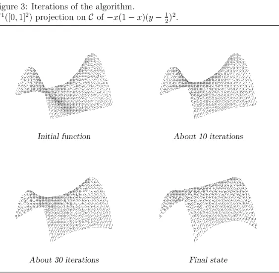
Figure 3: Iterations of the algorithm.
H1([0, 1]2) projection on C of −x(1 − x)(y − 1 2)2.
Initial function About 10 iterations
About 30 iterations Final state
of a finite number of affine constraints on the values zi = u(Min), since then
the functional can be expressed as a quadratic form of the (zi), using standard
relations in numerical analysis. The minimization of a quadratic functional in a set defined as the intersection of a finite number of hyperplanes is called ‘quadratic programming’, and is very classical in the literature.
In the following, we will use some useful notations for points in R2. We
note [A, B, C] := co{A, B, C} the closed triangle generated by three points. We recall that the area of this triangle is half the absolute value of
[A : B : C] := (B − A) ∧ (C − A)
= (xB− xA)(yC− yA) − (xC − xA)(yB− yA).
coordinates with respect to this triangle: α(M ) := ¯ ¯ ¯ ¯ [M : B : C] [A : B : C] ¯ ¯ ¯ ¯ , β(M) := ¯ ¯ ¯ ¯ [M : C : A] [A : B : C] ¯ ¯ ¯ ¯ , γ(M) := ¯ ¯ ¯ ¯ [M : A : B] [A : B : C] ¯ ¯ ¯ ¯ . They sum to 1 and
M = αA + βB + γC. (13) If [A : B : C] = 0, that is for instance B ∈ [A, C], we extend this defini-tion by setting for instance β = 0, α = AM/AC, γ = M C/AC, so that (13) remains valid. (The barycentric coordinates are not unique in this degenerate case.)
A first characterization of cone Cn is given by:
Theorem 2 Let u ∈ En and zi = u(Min). Then u ∈ Cn if and only if, for
all i, j, k, l ∈ (Nn)4 such that Min ∈ [Mjn, Mkn, Mln], we have
zi ≤ α(Min)zj + β(Min)zk+ γ(Min)zl (14)
where α, β, γ are the barycentric coordinates in [Mn
j, Mkn, Mln].
Note that even if the barycentric coordinates are not unique (for instance if k = l), they all give the same right member in (14).
Proof. If u = In(v), with v ∈ C, we have zi = v(Min). Since v is convex,
(14) follows immediately.
Let us prove that (14) implies that u ∈ Cn. Consider Pi := (xni, yni, zi) ∈
R3, Q
0 the convex hull of {Pi}i∈Nn inR
3 and
Q :=[
t≥0
(Q0+ te3)
where e3 := (0, 0, 1). It is easy to check that Q is a closed convex unbounded
subset ofR3 whose extremal points are included in {Pi}i∈Nn and having the
graph property: there exists a function v :R2 → R ∪ {+∞} such that
Q =©(x, y, z) ∈ R3 : z ≥ v(x, y)ª.
Notice that v is convex since its epigraph Q is convex. Moreover, if D ⊂ Ω is the projection of Q0 onto R2, we see that D is the union of all triangles
of Tn, and that v(M ) is finite if and only if M ∈ D. The restriction of v
(since Q0 is a polyhedron); hence, there exists a convex function w ∈ C such
that v ≡ w in D.
We claim that Pi ∈ ∂Q for all i. For if not, we can find i such that Pi is an
interior point of Q, that is zi > v(xni, yin). Since the point (xin, yni, v(xni, yni))
is in ∂Q, it belongs to a two-dimensional face of Q; from Caratheodory’s theorem, it belongs to a triangle of extremal points [Pj, Pk, Pl]; in particular
by projection, Mn
i ∈ [Mjn, Mkn, Mln]. Notice that we have v(xnj, yjn) = zj and
similar relations hold for k, l, since Pj, Pk, Pl are extremal. Let α, β, γ some
barycentric coordinates for Mn
i in [Mjn, Mkn, Mln]; we then have:
αzj + βzk+ γzl = v(xni, yin) < zi
and this contradicts (14).
Hence zi = v(Min) = w(Min) for all i. This implies that u = In(w) ∈ Cn
and the proof is complete.
As a consequence, problem (5) turns out to be finite dimensional quadra-tic programming problem for which the set of linear constraints is given by the previous proposition. Unfortunately, the number of constraints in (14) is of order O(k4
n), which is very large. But there are plenty of redundancies
in those relations:
Theorem 3 Under the same assumptions than in Theorem 2, u ∈ Cn if and
only if (14) is satisfied for all indices (i, j, k, l) such that Mn
i ∈ [Mjn, Mkn, Mln]
and
∀p /∈ {i, j, k, l}, Mpn ∈ [M/ jn, Mkn, Mln]. (15)
Moreover, this characterization is optimal in the following sense: if the indices (i0, j0, k0, l0) satisfy (15), there exists u0 ∈ En such that u0 ∈ C/ n, u0
satisfy (14) for all indices (i, j, k, l) 6= (i0, j0, k0, l0) satisfying (15).
We will give the proof below, but let us first give some consequences. We note that, if Mn
j, Mkn, Mln are non aligned, the additional condition (15)
expresses that Mn
i is the only vertex of Tn in the non-extremal points of the
triangle. Up to permutations, the only other case is k = l, and then (15) expresses that Mn
i is the only vertex in (Mjn, Mkn).
These conditions appear to be very simple for a structured mesh:
Corollary 4 Assume that for some n, Tn is a structured mesh, that is,
{Min}i∈Nn = Ω ∩ Z
2
u(α) = +∞ for all α ∈ Z2 \ M. Then u ∈ C
n if and only if, for all
α = (α1, α2) ∈ M we have:
∀(σ1, σ2) ∈ {−1, +1}2,
u(α) ≤ 1
3[u(α1+ σ1, α2) + u(α1, α2+ σ2) + u(α1− σ1, α2− σ2)]
(16)
and
u(α) ≤ 12[u(α + β) + u(α − β)] (17)
for all β ∈ Z2 such that either β = (0, 1), or β = (1, 0), or β = (±k, l) where
k ≥ 1, l ≥ 1 are integers satisfying k ∧ l = 1.
This follows from Theorem 3 by observing that, if three points of Z2 are
aligned, but their segment does not contain any other point ofZ2, then they
have the form α, α + β, α − β with β as described in the corollary. And if a triangle ofZ2 contains only α ∈ Z2 in its interior or boundary (except for
the vertices), it has the form [(α1 + σ1, α2), (α1, α2 + σ2), (α1− σ1, α2 − σ2)]
with (σ1, σ2) ∈ {−1, +1}2; in this case, the barycentric coordinates of α are
equal.
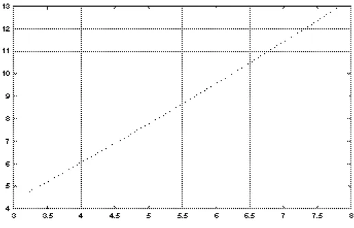
Hence, for a structured mesh with kn vertices, the number of constraints
is of order k1.8
n approximately (see Figure 4).
Proof of Theorem 3.
In this proof, n is constant; we drop upperscript n for simplicity. We note G :=n(i, j, k, l) ∈ N4: Mi ∈ [Mj, Mk, Ml] \ {Mj, Mk, Ml}
o .
We assume that (14) is satisfied for all indices (i, j, k, l) ∈ G such that (15) is satisfied. We would like to prove it for all other (i, j, k, l) ∈ G. The case k = l (corresponding to one-dimensional simplexes) is easy: the restriction of a convex function on a line has a monotone derivative, so the property (14) has just to be verified for three consecutive points on the same line.
Hence we just have to consider two-dimensional simplexes. In order to shorten notations, we will write
[i : j : k] := (Mj− Mi) ∧ (Mk− Mi).
We note for further reference the algebraic identity, valid for all (i, j, k, l, p): [i : p : j] [i : k : l] + [i : j : k] [p : l : i] = [i : k : p] [i : l : j]. (18)
Figure 4: Graph of the number of constraints C with respect to the total number of points N in the mesh, in log-log scale. A law in the form C ' N1.8
appears.
Let G0 ⊂ G be the set of indices (i, j, k, l) satisfying (14). If we assume
that G0 6= G, then we can find (i, j, k, l) ∈ G \ G0 such that [Mj, Mk, Ml] has
the smaller area. We then have (assuming that [Mj, Mk, Ml] is direct):
[j : k : l]zi > [i : k : l]zj + [i : l : j]zk+ [i : j : k]zl. (19)
By assumption, (15) is not satified for (i, j, k, l): hence, there exists p /∈ {i, j, k, l} such that Mp ∈ [Mj, Mk, Ml]. We can even assume that Mp ∈
[Mi, Mk, Ml] for instance, up to a permutation of the indices j, k, l. Since
the area of [Mi, Mk, Ml] is smaller than the area of [Mj, Mk, Ml], we have
(p, i, k, l) ∈ G0:
[i : k : l]zp ≤ [p : k : l]zi+ [p : l : i]zk+ [p : i : k]zl. (20)
Since Mp ∈ [Mi, Mk, Ml], and
Mi ∈ [Mj, Mk, Ml] = [Mp, Mk, Ml] ∪ [Mj, Mp, Ml] ∪ [Mj, Mk, Mp]
we must have Mi ∈ [Mj, Mp, Ml] or Mi ∈ [Mj, Mk, Mp]. We assume the
case it is positive), since if Mi, Mk, Mp are aligned, they must also be aligned
with Ml. And then this reduces to the case of one-dimensional simplexes.
Again, we must have (i, j, k, p) ∈ G0 since the area of [Mj, Mk, Mp] is
smaller than the area of [Mj, Mk, Ml]:
[p : j : k]zi ≤ [i : k : p]zj+ [i : p : j]zk+ [i : j : k]zp. (21)
Mutliplying this relation by [i : k : l] and using (20), we get [i : k : l] [p : j : k]zi ≤ [i : k : l] [i : k : p]zj + [i : k : l] [i : p : j]zk+
+ [i : j : k]³[p : k : l]zi+ [p : l : i]zk+ [p : i : k]zl
´
≤ [i : k : l] [i : k : p]zj + [i : k : p] [i : l : j]zk+
+ [i : j : k] [i : k : p]zl+ [i : j : k] [p : k : l]zi
taking (18) into account.
Exchanging k and i in (18), we get:
[p : j : k] [i : k : l] − [i : j : k] [p : k : l] = [i : k : p] [j : k : l] so that the preceding inequality can be rewritten:
[i : k : p] [j : k : l]zi ≤ [i : k : p]
³
[i : k : l]zj+ [i : l : j]zk+ [i : j : k]zl
´ . This contradicts (19) since [i : k : p] > 0. Hence, we have G0 = G and the
proof of the first part is complete.
We now prove our assertion on the optimality. If (i0, j0, k0, l0) ∈ G
satis-fies (15), we can find a compact convex set K such that K ∩ {Mi}i=1,...,kn = {Mi0, Mj0, Mk0, Ml0}
and Mi0 is an interior point of K. Let v be any convex function satisfying
v ≡ 0 in K and v > 0 in R2\ K.
For instance the function v(M ) = dist(M, K) is convenient. Since v is con-tinuous and K is compact,
min
p /∈{i0,j0,k0,l0}
v(Mp) > 0.
Hence there exists ε > 0 such that for all indices (j, k, l) 6= (j0, k0, l0) (up to
permutations) satisfying (i0, j, k, l) ∈ G, we have
where α, β, γ are the barycentric coordinates of Mi0 in [Mj, Mk, Ml] (indeed,
max(α, β, γ) is bounded from below as (j, k, l) changes, since Mi0 is an interior
point of K).
Consider the function u ∈ En satisfying u(Mp) = v(Mp) for all p 6= i0 and
u(Mi0) = ε. If (i, j, k, l) ∈ G, with i 6= i0, we have
u(Mi) = v(Mi) ≤ α(Mi)v(Mj) + β(Mi)v(Mk) + γ(Mi)v(Ml)
≤ α(Mi)u(Mj) + β(Mi)u(Mk) + γ(Mi)u(Ml)
using the convexity of v and u ≥ v at every node. Hence u satisfies (14) for these indices.
Also if (j, k, l) 6= (j0, k0, l0) (up to permutations) satisfies (i0, j, k, l) ∈ G,
then u satisfies (14) from the definition of ε in (22).
We conclude that u satisfies all constraints with indices (i, j, k, l) 6= (i0, j0, k0, l0), but it is not in Cn since
u(Mi0) = ε > 0 = α(Mi0)v(Mj0) + β(Mi0)v(Mk0) + γ(Mi0)v(Ml0).
This ends the proof of the proposition.
4
Convexification and projection
Let u0 be some function in H01(Ω) and f = ∆u0. We will prove in this section
that the solution ΠC(u0) of the minimization problem in K = H01(Ω) with
J = Jf (as defined in (2)) is, in general, different from u∗∗0 (which is the
minimizer of Ju0 defined in (3) on Ku0).
Theorem 5 We have u∗∗
0 = ΠC(u0) if and only if
h∆u∗∗0 , u0− u∗∗0 i = 0. (23)
As a consequence, in dimension 1, we always have u∗∗
0 = ΠC(u0) since (23) is
always satisfied. However, this is not true in higher dimensions (see remark hereafter).
Proof. Assume first that u∗∗
0 is a minimizer of Jf in H01(Ω). Then for all
convex v with v = 0 in ∂Ω, Jf0(u∗∗0 ), v − u∗∗0
®
≥ 0. Taking v = 0 here yields: h∆(u0− u∗∗0 ), u∗∗0 i = h∆u∗∗0 , u0− u∗∗0 i ≤ 0.
Conversely assume (23), then for all h ∈ H1
0(Ω) such that u∗∗0 + h is
convex, the following holds:
Jf(u∗∗0 + h) − Jf(u∗∗0 ) ≥ Jf0(u∗∗0 ), h® = Z Ω∇u ∗∗ 0 · ∇h + h∆u0 = h∆(u0− u∗∗0 ), hi writing h = v − u∗∗
0 with v ∈ H01(Ω) ∩ C in the latter and using (23) yields:
Jf(v) − Jf(u∗∗0 ) ≥ h∆(u0− u∗∗0 ), vi = h∆v, u0− u∗∗0 i ≥ 0
which proves that u∗∗
0 minimizes Jf over H01(Ω) ∩ C.
Remark. Condition (23) indicates that for almost every x ∈ Ω, we have either u0(x) = u∗∗0 (x) or ∇u∗∗0 ≡ const. in a neighborhood of x. For instance,
if Ω is the unit ball ofR2, and u
0(x) = |x|3−|x|, we have u∗∗0 = min(−3√23, u0)
and (23) is satisfied.
On the other hand, if u0(x) =
p |x| − 1, then u∗∗ 0 (x) = |x| − 1 and (23) is not satisfied.
5
Numerical solution
5.1
Algorithm
We consider a structured triangulation of the unit square [0, 1] × [0, 1] = Ω. Any function u ∈ Cn can be written
u =
kn
X
i=1
uiwi,
where (wi) is the standard basis of En (wi(Mj) = δij). In what follows, u
will represent both the function of En and the vector of its components in
this basis. The stiffness matrix A = (aij) is defined by
aij=
Z
Ω∇w
i· ∇wj.
Let m be the number of constraints. The set of feasible states (see corollary 4) can be written
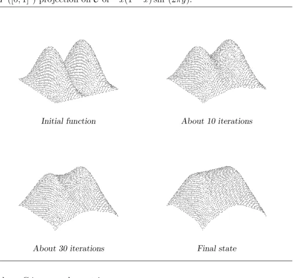
Figure 5: Iterations of the algorithm.
H1([0, 1]2) projection on C of −x(1 − x) sin2(2πy).
Initial function About 10 iterations
About 30 iterations Final state
where C is a m × kn matrix.
We finally end up with a classical quadratic programming problem: Find u ∈ Cn such that
J(u) = 1
2(Au, u) + (b, u) = minv∈Cn
J (v) (25) We propose to solve this problem by a Uzawa-like algorithm [1]. The initial problem is replaced by the following: Find a saddle point for the Lagrangian defined for (u, λ) ∈ Rkn × Rm
+ by
L(v, λ) = 1
2(Av, u) + (b, v) + (λ, Cv). (26) We denote by Π+ the projection ontoRm
+.
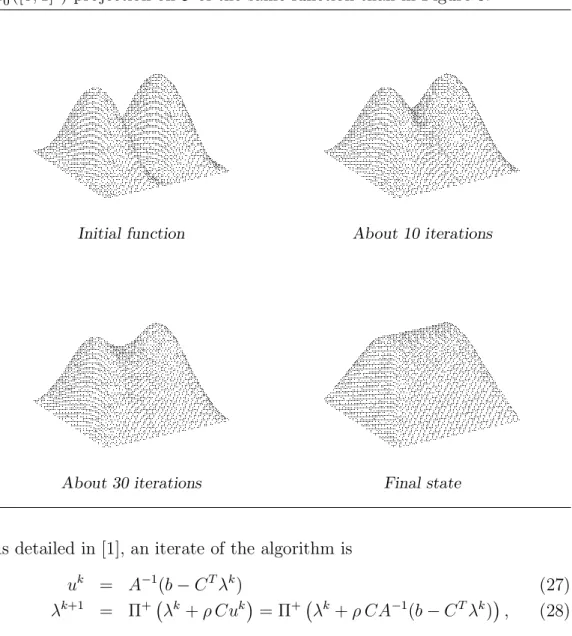
Figure 6: Iterations of the algorithm. H1
0([0, 1]2) projection on C of the same function than in Figure 5.
Initial function About 10 iterations
About 30 iterations Final state
As detailed in [1], an iterate of the algorithm is
uk = A−1(b − CTλk) (27) λk+1 = Π+¡λk+ ρ Cuk¢= Π+¡λk+ ρ CA−1(b − CTλk)¢, (28) where ρ > 0 is the step parameter (see next section).
5.2
Numerical parameters
Weighting of the constraints
From a theorical point of view, the initial problem remains the same if any constraint (row of C) is multiplied by any positive number, whereas the behaviour of the algorithm is likely to vary. Indeed, matrix C can be replaced by DC, where D is a diagonal m × m matrix with positive elements. Note
that, as problem (26) does not admit a unique solution in λ since m > kn, it
may change completely the behaviour of the sequence (λk).
The choice we propose here is based on the following heuristic: given a field u ∈ En, we would like the m-dimensional vector DCu to be related to
the distance between u and the set of convex functions. Using notations of corollary 4, we define δαβ(u) for any u ∈ En by
δαβ(u) = 2u(α) − u(α − β) − u(α + β)
2 |β|2 , (29)
where β = (β1, β2) ∈ Z2, |β|2 = β12+ β22, and
∆ασ(u) = 3u(α) − u(α1
+ σ1, α2) − u(α1, α2+ σ2) − u(α − σ)
4 , (30)
where σ = (σ1, σ2) ∈ {−1, +1}2, and we introduce the number
η(u) = max(0, max
α,β δαβ(u), maxα,σ ∆ασ(u)). (31)
We have the following proposition:
Proposition 3 A function u ∈ En is in Cn if and only if η(u) ≤ 0.
Furthermore, for any norm k k on En, there exists a constant K such that,
∀u ∈ En, dist(u, Cn) = inf
v∈Cnku − vk ≤ Kk
nη(u). (32)
Proof. The first part is a direct consequence of corollary 4: all constraints have been multiplied by a positive number.
Let h be the mesh size, which verifies h2 ' 1/k
n for n large. Let us now
define Λ ∈ Cn as the interpolate of the quadratic function (x, y) 7−→ x2+ y2.
A straightforward calculation shows that δαβ(u + η h2Λ) ≤ 0 ∀α, β, (33) and ∆ασ(u + η h2Λ) ≤ 0 ∀α, σ, (34) so that u + hη2Λ ∈ Cn. (Actually η
h2 is the smallest number τ such that
u + τ Λ ∈ Cn.) Therefore, dist(u, Cn) = inf v∈Cnku − vk ≤ ° ° °u − (u + hη2Λ) ° ° ° = hη2 kΛk , (35)
which ends the proof, with K = kΛk.
The matrix C we used in computations is the algebraic form of the scaled constraints δαβ(u) ≤ 0, ∆ασ(u) ≤ 0, for all α, β, and σ.
Choice of ρ
Let α be the smallest eigenvalue of A. It is shown in [1] that the algorithm converges for any ρ ∈ (0, ρ0
c), with ρ0c = 2α/kCk2. We propose a sharper
upperbound ρ1 c ≥ ρ0c,
ρ1c = 2
kCA−1CTk, (36)
for which convergence can be established as well. This critical value ρ1 c can
be estimated numerically, using the fact that CA−1CT is symmetric, so that
the 2-norm is the spectral radius.
It turns out to be much larger than ρ0
c, leading to a faster converging
algorithm. Furthermore, ρ1
c appears to be close to optimal, as the algorithm
diverges as soon as ρ ≥ 1.1 × ρ1 c.
Remark. The inequality ρ1
c À ρ0c is due to
kCA−1CTk ¿ kCk kA−1k kCTk, (37) which is closely related to the nature of the problem we solve. More precisely, as the rows of C correspond to second order derivatives, CTC is spectrally close to the discrete bilaplacian operator, which is basically A2. Let us denote
by 0 < α1 < · · · < αkn the eigenvalues of A. The smallest eigenvalue verifies
α1 ∼ 2π2h2, where h is the mesh size, and αkn is a O(1). Considering the
idealized situation CTC = A, one can check easily that the spectrum of
CA−1CT is the spectrum of A plus the eigenvalue 0 with multiplicity m − k n,
so that kCA−1CTk is O(1). Besides the right-hand side of (37) is α2 kn/α1,
which is a O(1/h2). We therefore have
ρ0c = O(h2) , ρ1c = O(1). (38) We checked numerically that these estimates hold for the actual matrices, and not only in the simplified situation CTC = A.
Some results of the computations are shown in Figures 1–3, 5–6. For the clearness of the pictures, the z-axis is directed downward in these figures.
References
[1] P. G. Ciarlet, Introduction a` l’analyse nume´rique matricielle et a` l’optimisation, Collection mathe´matiques applique´es pour la Maıˆtrise, Masson Paris (1982).
[2] P. Chone´, E´tude de quelques proble`mes variationnels intervenant en ge´ome´trie riemannienne et en e´conomie mathe´matique, PhD Thesis, Univ. Toulouse I (1999).
[3] I. Ekeland, R. Temam, Convex Analysis and Variational Problems, North-Holland (1972).
[4] J.-C. Rochet, P. Chone´, Ironing, Sweeping and Multidimensional screening, Econometrica 66 (1998), pp. 783–826.