Optimal Portfolio Liquidation with Limit Orders
Olivier Guéant, Charles-Albert Lehalle, Joaquin Fernandez Tapia
Les Cahiers de la Chaire / N°44
Optimal Portfolio Liquidation with Limit Orders
Olivier Gu´
eant
∗, Charles-Albert Lehalle
∗∗, Joaquin Fernandez Tapia
∗∗∗May 2011
Abstract
This paper addresses the optimal scheduling of the liquidation of a portfolio using a new angle. Instead of focusing only on the scheduling aspect like Almgren and Chriss in [2], or only on the liquidity-consuming orders like Obizhaeva and Wang in [31], we link the optimal trade-schedule to the price of the limit orders that have to be sent to the limit order book to optimally liquidate a portfolio. Most practitioners address these two issues separately: they compute an optimal trading curve and they then send orders to the markets to try to follow it. The results obtained here solve simultaneously the two problems. As in a previous paper that solved the “intra-day market making problem” [19], the interactions of limit orders with the market are modeled via a Poisson process pegged to a diffusive “fair price” and a Hamilton-Jacobi-Bellman equation is used to solve the trade-off between execution risk and price risk. Backtests are finally carried out to exemplify the use of our results.
Introduction
Optimal scheduling of large orders in order to control the overall trading costs with a trade-off between market impact (demanding to trade slow) and market risk (urging to trade fast) has been proposed in the litterature in the late nineties mainly by Bertsimas and Lo [8] and Almgren and Chriss [2]. If the original approach has been recently generalized in several directions (see for instance [3, 4, 13, 14, 15, 18, 26, 29, 34]), only few attempts have been made to drill down the model at the level of the interactions with the order books. The more noticeable proposal is the one by Obizhaeva and Wang [31], followed and sophisticated by Alfonsi, Fruth and Schied [1] or Predoiu, Shaikhet and Shreve [33]. This branch of the optimal trading literature1 focuses on the dynamics initiated by aggressive orders hitting a
martingale and resilient order-book2, ignoring then trading by passive orders.
Just recall that during the continuous auction processes implemented by most electronic trading pools, market participants send their open interests (i.e. buy or sell orders) to a queuing system where a “first in first out” queue stands at each possible price. If a buy (respectively sell) order reaches a queue of sell (resp. buy) orders, a transaction occurs (see for instance [28] for more explanations and modelings). Orders generating trades are said
The authors wish to acknowledge the helpful conversations with Vincent Fardeau (LSE), Jean-Michel Lasry (Universit´e Paris-Dauphine), Gilles Pag`es (Universit´e Pierre et Marie Curie), Nizar Touzi (Ecole Polytechnique).
∗UFR de Math´ematiques, Laboratoire Jacques-Louis Lions, Universit´e Paris-Diderot. 175, rue du Chevaleret,
75013 Paris, France. [email protected]
∗∗Head of Quantitative Research. Cr´edit Agricole Cheuvreux. 9, Quai du Pr´esident Paul Doumer, 92400
Courbevoie, France. [email protected]
∗∗∗PhD student, Universit´e Pierre et Marie Curie. 4 place Jussieu, 75005 Paris, France. 1see also [10, 20, 23, 24] for different approaches.
to be aggressive or liquidity-consuming ones; orders filling queues are said to be passive or liquidity-providing ones. In practice, most trading algorithms are as passive as possible (a typical balance for a scheduling algorithm is around 60% of passively obtained trades – see [27]).
The economic literature first explored and studied these interactions between orders sent to a continuous auction system by different actors from a global efficiency viewpoint3.
With the fragmentation of equity markets in the US and in Europe, the issue of linking optimal posting prices to the optimal liquidation of a portfolio is more and more important. A trading algorithm has to find an optimal scheduling or rhythm for its trading, but also to choose a sequel of prices and quantities of orders to send to the markets to follow this optimal rhythm as much as possible.
This paper answers this “optimal scheduling and posting” problem as a whole. Indeed, and in contrast with most of the preceding literature4, we propose a new approach which is liquidity-providing oriented: liquidation strategies involve limit orders and not only market orders. As a consequence, the classical trade-off of the literature between market impact, or execution costs, and price risk disappears in our setting since no execution cost is incurred. However, since the broker does not know when his orders are going to be executed – if at all –, a new risk is borne: (non-)execution risk. If a limit ask order is inserted in the order book, probability of execution and eventually time of execution will depend on the price of the order.
In our framework, the flow of the trades “hitting” a passive order at a distance δ from the “fair price” St (modeled by a Brownian Motion) follows an adapted Poisson process of
in-tensity A exp(−kδ). It means that the further away from the “fair price” an order is posted, the less transactions it will obtain. If the limit order price is far above the best ask price, the trading gain may be high but execution is not guaranteed and the broker is exposed to the risk of a price decrease. On the contrary, if the limit order price is near the best ask price, or even reduces the market bid-ask spread, gains will be small but the probability of execution will be higher, resulting in faster trading and less price risk.
Our modeling paradigm for optimal liquidation is in fact rooted to recent works in other areas of algorithmic trading. Market making models developed by Ho and Stoll [21] or more recently by Avellaneda and Stoikov [5] for “high frequency market making in an order-book” are instances of the use of limit orders in the financial literature. Our approach is more pre-cisely inspired from the resolution of the “market making” problem in a companion paper [19].
The main limitations of our models are twofold. First, our framework deals with one trading venue only. Hence we do not model a “smart order routing” (SOR) mechanism but it can be seen as the consolidation of all available trading venues, without taking directly into account the potential specificity of each of them5.
Second, market impact is not modeled in our framework, be it permanent or transient. In previous works on optimal trade scheduling, market impact was typically rendered by an explicit model because trading was done with liquidity-consuming orders. The same kind of assumptions could have been made on executed orders but, the introduction of limit orders in the literature on optimal trading being quite recent, there is still no model for the market impact of liquidity-providing orders.
3see [16] for a study of the effect of “smart order routing” on competitive trading venues, or [9] for a study of
the efficiency of order matching mechanisms.
4Kratz and Sch¨oneborn [25] proposed an approach with both market orders and access to dark pools.
5The actual models studying the SOR problem across several venues are more focused on routing across Dark
To the authors’ knowledge, it is indeed the first proposal to drill down to passive orders modeling to solve the optimal trade scheduling for large orders6. It is organized as follows:
in the first part, we present the setting of the model and the main hypotheses on execution. The second part is devoted to the resolution of the partial differential equations arising from the control problem. Part 3, deals with two special cases, namely the time-asymptotic case and the “no-volatility” benchmark that provide closed-form formulae. Then, in part 4, we carry out comparative statics and discuss the way optimal strategies depend on the model parameters. Part 5 generalizes the model to take account of different liquidation hypotheses and different sizes of orders. Finally, in part 6, we show how our approach can be used in practice for optimal liquidation.
1
Setup of the model
We consider a trader who has to liquidate a portfolio containing a large quantity q0 of a
given stock. We suppose that the reference price of the stock (that can be considered the mid-price or the best bid quote for example) moves as a brownian motion with a drift:
dSt= µdt + σdWt
The trader under consideration will continuously propose an ask quote denoted Staand will hence sell shares according to the rate of arrival of aggressive orders at the prices he quotes. His inventory q, that is the quantity he holds, is given by qt = q0 − Nta where Na is the
jump process giving the number of shares he sold. This jump process is supposed to be a Poisson process and to simplify the exposition we consider that jumps are of unitary size7. Arrival rates obviously depend on the price Sta quoted by the trader and we assume, in accordance with most datasets, that intensity λaassociated to Nais of the following form:
λa(sa, s) = A exp(−k(sa− s))
This means that the cheaper the order price, the faster it will be executed.
As a consequence of his trades, the trader has an amount of cash whose dynamics is given by:
dXt= StadNta
The trader has a time horizon T to liquidate the portfolio and his goal is to optimize the expected utility of his P&L at time T . We will focus on CARA utility functions and we suppose that the trader optimizes:
sup
Sa E [− exp (−γXT
) 1qT=0− ∞1qT̸=0]
where γ is the absolute risk aversion characterizing the trader, where XT is the amount of
cash at time T and where qT is the remaining quantity of shares in the inventory at time T .
This criterion forces the trader to use every endeavor to liquidate the portfolio. Less extreme criteria will be discussed in section 5.
6It recently came to our knowledge that a similar approach for liquidation with limit orders is being developed
independently by E. Bayraktar and M. Ludkovski [7]. Their approach uses the same framework as ours to describe the price process and the execution mechanism. However, they only consider risk-neutral traders and consequently they do not take account of risk, be it price risk, or execution risk.
7Alternatively, in part 5, we will consider that trades are of size δq. It’s important to notice that 1 share may
be understood as 1 bunch of shares, each bunch being of the same size, typically the average trade size (hereafter ATS) or a fraction of it.
2
Resolution
2.1
Hamilton-Jacobi-Bellman equation
The optimization problem set up in the preceding section can be solved using classical Bellman tools. To this purpose, we introduce a Bellman function u defined as:
u(t, x, q, s) = sup
Sa E [− exp (−γXT
) 1qT=0− ∞1qT>0| Xt= x, St= s, qt= q]
The Hamilton-Jacobi-Bellman equation associated to the optimization problem is then given by the following proposition:
Proposition 1 (HJB). The Hamilton-Jacobi-Bellman equation for u is:
(HJB) 0 = ∂tu(t, x, q, s) + µ∂su(t, x, q, s) + 1 2σ 2∂2 ssu(t, x, q, s) + sup sa λ a(sa, s) [u(t, x + sa, q− 1, s) − u(t, x, q, s)] with the final condition:
u(T, x, q, s) =− exp (−γx) 1q=0− ∞1q>0 and the boundary condition:
u(t, x, 0, s) =− exp (−γx)
To solve the Hamilton-Jacobi-Belmann equation, we will use a change of variables that transforms the PDEs in a system of linear ODEs.
Proposition 2 (A system of linear ODEs). Let’s consider a family of functions (wq)q∈N
solution of the linear system of ODEs (S) that follows:
∀q ∈ N, ˙wq(t) = (αq2− βq)wq(t)− ηwq−1(t)
with wq(T ) = 1q=0 and w0= 1, where α = k2γσ2, β = kµ and η = (1 +γk)−(1+ k γ).
Then u(t, x, q, s) =−A−γqk exp(−γ(x + qs))wq(t)− γ
k is solution of (HJB).
Now, using this system of ODEs, we end up with the optimal quotes:
Theorem 1 (Optimal quote). Let’s consider the solution w of the system (S) of Proposition
2. Then, the optimal ask quote can be expressed as:
sa∗(t, q, s) = s + ( 1 kln ( wq(t) wq−1(t) ) + 1 kln(A) + 1 γ ln ( 1 +γ k ))
Corollary 1 (Trading intensity). The trading intensity associated to the optimal strategy
does not depend on A.
Consequently if we define the trading curve as the average8 evolution of the inventory, i.e. V (t) :=E[qt], then t7→ V (t) does not depend on A.
8In our case indeed, since the execution process is not deterministic, the trading curve associated to the optimal
2.2
Numerical example
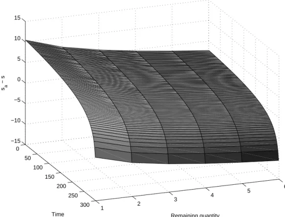
Proposition 2 and Theorem 1 provide a way to solve the Hamilton-Jacobi-Bellman equation and to derive the optimal quotes for a trader willing to liquidate a portfolio. To exemplify these results we compute the optimal quotes when a quantity of shares up to 6 times the ATS has to be sold within 5 minutes (Figure 1).
0 50 100 150 200 250 300 1 2 3 4 5 6 −15 −10 −5 0 5 10 15 Remaining quantity Time s a − s
Figure 1: Optimal strategy sa∗(t, q)− s (in Ticks) for an agent willing to sell a quantity of shares up to 6 times the ATS within 5 minutes (µ = 0 (Tick.s−1), σ = 0.3 (Tick.s−12), A = 0.1 (s−1), k = 0.3 (Tick−1)
and γ = 0.05 (Tick−1))
We clearly see that the optimal quotes depend on time and inventory in a monotonic way. Indeed, a trader with a lot of shares to get rid of wants to trade fast and will therefore propose a low price. On the contrary a trader with only a few shares in his portfolio may be willing to benefit from a trading opportunity and will send an order with a higher price because the risk he bears allows him to trade more slowly.
Now, coming to the time-dependence of the quotes, a trader with a given number of shares will, ceteris paribus, lower his quotes as the time horizon gets closer. At the limit when t is close to the time horizon T , the optimal quotes tends to −∞. In practice very negative values for the ask quotes have to be understood as market orders on the bid side.
Also, we see that optimal quotes have an asymptotic behavior as time horizon increases. The associated limiting case will be studied in depth in the next section.
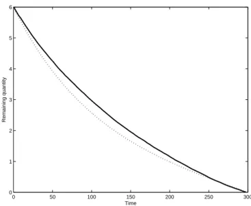
Finally, the trading curve associated to the above optimal quotes can be obtained by Monte-Carlo simulations as exemplified on Figure 2.
0 50 100 150 200 250 300 0 1 2 3 4 5 6 Time Remaining quantity
Figure 2: Solid line: Trading curve for an agent willing to sell a quantity of shares equal to 6 times the ATS within 5 minutes (µ = 0 (Tick.s−1), σ = 0.3 (Tick.s−12), A = 0.1 (s−1), k = 0.3 (Tick−1) and
γ = 0.05 (Tick−1)). Dotted line: Trading curve calculated using the Almgren-Chriss framework with the same parameters and the impact function f (v) = 20v1+34.
3
Special cases
The above equations can be solved explicitly for w and hence for the optimal quotes. How-ever, the resulting closed-form expressions are not really tractable and do not provide any intuition on the behavior of the optimal quotes. Two special cases are now considered for which simple closed-form formulae can be derived. We start first with the limiting behavior of the quotes, when the time horizon T tends to infinity. We then consider a benchmark case in which there is no volatility (σ = 0) as an approximation for low-volatility cases.
3.1
Asymptotic behavior as T
→ +∞
We have seen on Figure 1 that the optimal quotes seem to exhibit an asymptotic behavior. We are in fact going to prove that sa∗(0, q, s) tends to a limit as the time horizon T tends to infinity.
Proposition 3 (Asymptotic behavior of the optimal quotes). Let’s suppose that9 γσµ2 < 12.
Let’s consider the solution w of the system (S) of Proposition 2. Then:
lim T→+∞wq(0) = ηq q! q ∏ j=1 1 αj− β
The resulting asymptotic behavior for the optimal ask quote of Theorem 1 is:
lim T→+∞s a∗(0, q, s) = s + 1 kln ( A 1 +γk 1 αq2− βq )
3.2
The “no-volatility” benchmark
Though unrealistic, we now concentrate on a benchmark case in which there is no volatility (σ = 0). In that benchmark case, the trader bears no price risk and the only risk he faces is linked to the non-execution of his orders.
In this framework, we can derive tractable formulae for the optimal quotes. By analogy with the initial literature on optimal liquidation [2], we can also obtain analytical expressions for trading curves.
Proposition 4 (The “no-volatility” benchmark). Let’s first consider µ̸= 0.
wq(t) = η q q! ( eβ(T−t)−1 β )q
defines a solution of the system (S). The optimal quote is
sa∗(t, q, s) = s + ( 1 kln ( η q eβ(T−t)− 1 β ) +1 kln(A) + 1 γ ln ( 1 +γ k ))
that can also be written:
sa∗(t, q, s) = s +1 kln ( A 1 +γk 1 q eβ(T−t)− 1 β )
The associated trading curve is Vt= q0
(
1−e−β(T −t) 1−e−βT
)1+γk
.
In the absence of a drift (µ = 0, σ = 0), similar formulae can be obtained:
Corollary 2 (The “no-volatility” benchmark – no-drift case). In the limit case µ = 0,
wq(t) = η
q
q!(T − t)q defines a solution of the system (S). The optimal quote is
sa∗(t, q, s) = s + ( 1 kln ( η q(T − t) ) + 1 kln(A) + 1 γln ( 1 +γ k ))
that can also be written:
sa∗(t, q, s) = s +1 kln ( A 1 +γk T − t q )
The associated trading curve is V (t) = q0
(
1−Tt)1+
γ k.
4
Comparative statics
4.1
Intuition from the above cases
Before going to comparative statics in the general case, we focus on the particular cases for which tractable closed form formulae have just been derived. These closed-form formulae provide an approximation for the optimal quotes and trading curves respectively when t is far from T and when volatility is small. Hence, we can start to discuss the role played by the different parameters in these contexts.
Focusing first on the optimal quotes, we see both in the asymptotic case and in the “no-volatility” benchmark case that, quite naturally, the optimal ask quote is an increasing function of A. When trading intensity is high, many trades occur and a limit order inserted far above the reference price has indeed a large probability to be executed.
Risk aversion also plays an important role. Both in the asymptotic case and in the “no-volatility” benchmark case (also this last one misses part of the picture, ignoring price risk), a very risk-adverse agent will indeed be willing to reduce execution risk and will submit orders at low price.
Now, as far as k is concerned, the dependence of the optimal quote on k is ambiguous because the interpretation of k depends on the optimal quote itself. An increase in k corresponds
indeed to a decrease in the probability to be executed for prices above the reference price. However, due to the exponential form for execution intensity, the exact opposite is true for quotes below reference price, an increase in k implying an increase in the probability to be executed for quotes below reference price.
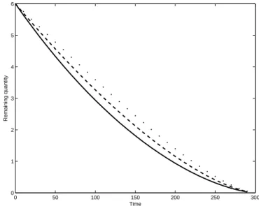
Now, turning to the trading curve in the “no-volatility” benchmark case, we see that the agent trades fast when risk aversion γ is large or when k is small. This is clearly instanced by Figure 3. 0 50 100 150 200 250 300 0 1 2 3 4 5 6 Time Remaining quantity
Figure 3: Trading curves of an agent willing to sell 6 times the ATS for different sets of parameters (in the no-drift case). Dots: risk neutral case γ = 0. Dotted line: k = 0.3 (Tick−1), γ = 0.05 (Tick−1). Solid line: k = 0.2 (Tick−1), γ = 0.1 (Tick−1)
Also, the agent trades faster when the price is expected to decrease to avoid selling at low price. This is clearly instanced by Figure 4.
0 50 100 150 200 250 300 0 1 2 3 4 5 6 Time Remaining quantity
Figure 4: Trading curves of an agent willing to sell 6 times the ATS for different values of the drift.
µ = 1/150 (Tick.s−1) (dots), µ = 0 (Tick.s−1) (dotted line), µ = −1/150 (Tick.s−1) (solid line) k = 0.2 (Tick−1), γ = 0.1 (Tick−1)
4.2
General case
Now, let’s turn to the general case to take account of volatility and thus of the price risk dimension of the problem.
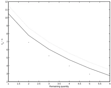
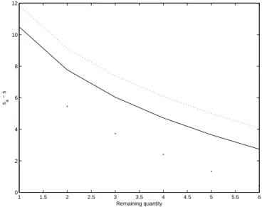
As far as the drift is concerned, quotes are naturally increasing with µ. If indeed the trader expects the price to move down, he is going to send orders at low prices to be executed fast and thus reduce the risk to suffer from the decrease in price. This is well exemplified in Figure 5. 1 1.5 2 2.5 3 3.5 4 4.5 5 5.5 6 2 3 4 5 6 7 8 9 10 11 12 Remaining quantity sa − s
Figure 5: Dependence on µ of sa∗(q)− s for an agent willing to sell a quantity of shares up to 6 times the ATS in the next 5 minutes. (µ = −1/150 (Tick.s−1) (dots), µ = 0 (Tick.s−1) (dotted line), µ = 1/150 (Tick.s−1) (solid line), σ = 0.3 (Tick.s−12), A = 0.1 (s−1), k = 0.3 (Tick−1) and γ = 0.05 (Tick−1))
Now, coming to volatility, the optimal quotes depend on σ in a monotonic way. If there is an increase in volatility, the price risk increases. In order to reduce this additional price risk the trader will send orders at cheaper price. This is what we observe numerically on Figure 6.
1 1.5 2 2.5 3 3.5 4 4.5 5 5.5 6 −2 0 2 4 6 8 10 12 Remaining quantity sa − s
Figure 6: Dependence on σ of sa∗(q)− s for an agent willing to sell a quantity of shares up to 6 times the ATS in the next 5 minutes. (µ = 0 (Tick.s−1), σ = 0 (Tick.s−12) (dots), σ = 0.3 (Tick.s−
1
2) (solid
Now, coming to A, we know that the optimal quotes are given by: sa∗(t, q, s) = s + ( 1 kln ( wq(t) wq−1(t) ) + 1 kln(A) + 1 γ ln ( 1 +γ k ))
Since w is independent of A, the optimal quotes increase with A as in the “no-volatility” benchmark case. Numerically, we indeed observe that the optimal quote is an increasing function of A (see Figure 7).
1 1.5 2 2.5 3 3.5 4 4.5 5 5.5 6 0 2 4 6 8 10 12 Remaining quantity sa − s
Figure 7: Dependence on A of sa∗(q)−s for an agent willing to sell a quantity of shares up to 6 times the ATS in the next 5 minutes. (µ = 0 (Tick.s−1), σ = 0.3 (Tick.s−12), A = 0.05 (s−1) (dots), A = 0.10 (s−1)
(solid line), A = 0.15 (s−1) (dotted line), k = 0.3 (Tick−1) and γ = 0.05 (Tick−1))
Then as far as the dependence of the optimal quotes on k is concerned, the above dis-cussion on the interpretation of k is still valid. Since high volatility may more often induce optimal quotes below the reference price, the dependence on k is not the same at all times and for all values of the inventory (Figure 8 and Figure 9).
1 1.5 2 2.5 3 3.5 4 4.5 5 5.5 6 0 2 4 6 8 10 12 14 16 Remaining quantity sa − s
Figure 8: Dependence on k of sa∗(q)− s for an agent willing to sell a quantity of shares up to 6 times the ATS in the next 5 minutes. (µ = 0 (Tick.s−1), σ = 0.3 (Tick.s−12), A = 0.10 (s−1), k = 0.2 (Tick−1)
1 1.5 2 2.5 3 3.5 4 4.5 5 5.5 6 −16 −14 −12 −10 −8 −6 −4 −2 0 2 4 Remaining quantity sa − s
Figure 9: Dependence on k of sa∗(q)− s for an agent willing to sell a quantity of shares up to 6 times the ATS in the next 5 minutes. (µ = 0 (Tick.s−1), σ = 3 (Tick.s−12), A = 0.10 (s−1), k = 0.2 (Tick−1)
(dots), k = 0.3 (Tick−1) (solid line), k = 0.4 (Tick−1) (dotted line) and γ = 0.05 (Tick−1))
Finally, turning to the risk aversion γ, two effects are at stake that go in the same direc-tion. The risk aversion is indeed common for both price risk and execution risk. Hence if risk aversion increases, the trader will try to reduce both price risk and execution risk, thus selling at cheaper price. We indeed see on Figure 10 that optimal quotes are decreasing in
γ. 1 1.5 2 2.5 3 3.5 4 4.5 5 5.5 6 0 2 4 6 8 10 12 Remaining quantity sa − s
Figure 10: Dependence on γ of sa∗(q)− s for an agent willing to sell a quantity of shares up to 6 times the ATS in the next 5 minutes. (µ = 0 (Tick.s−1), σ = 0.3 (Tick.s−12), A = 0.10 (s−1), k = 0.3 (Tick−1)
and γ = 0.01 (Tick−1) (dots), γ = 0.05 (Tick−1) (solid line), γ = 0.1 (Tick−1) (dotted line))
5
Different settings
5.1
Terminal condition
The above framework may seem quite extreme at first sight since a trader that does not liquidate his portfolio is supposed to incur a rather unrealistic infinite cost. However, our
model can be slightly changed to incorporate a less extreme penalization for not having liquidated one’s portfolio at time T .
Let’s consider indeed that the utility function of the agent is given by:
u(t, x, q, s) = sup
Sa E [− exp (−γ (XT
+ qTST − ϕ(qT)))| Xt= x, St= s, qt= q]
where ϕ : R → R is equal to +∞ for negative q’s (to avoid short selling) and is increasing for positive q’s with ϕ(0) = 0.
In this setting, the trader no longer incurs an infinite cost for not having liquidated his portfolio. Rather, we assume that he can sell the shares remaining at time T in his portfolio at a price below the reference price. The function ϕ(·) measures the liquidation discount with respect to the reference price.
In this new framework, we have results similar to those presented above. First, the Hamilton-Jacobi-Bellman equation associated to the optimization problem is given by the following proposition:
Proposition 5 (HJB). The Hamilton-Jacobi-Bellman equation for u is:
(HJB) 0 = ∂tu(t, x, q, s) + µ∂su(t, x, q, s) + 1 2σ 2∂2 ssu(t, x, q, s) + sup sa λ a(sa, s) [u(t, x + sa, q− 1, s) − u(t, x, q, s)] with the final condition:
u(T, x, q, s) =− exp (−γ (x + qs − ϕ(q))) and the boundary condition:
u(t, x, 0, s) =− exp (−γx)
We then use a similar change of variables to obtain the following proposition:
Proposition 6 (Change of variables and optimal quotes). Let’s consider a family of
func-tions (vq)q∈N solution of the linear system of ODEs (S) that follows: ∀q ∈ N, ˙vq(t) = (αq2− βq)vq(t)− ηAvq−1(t)
with vq(T ) = exp(−kϕ(q)) and v0= 1, where α = k2γσ2, β = kµ and η = (1 +γk)−(1+ k γ).
Then u(t, x, q, s) =− exp(−γ(x + qs))vq(t)−
γ
k is solution of (HJB).
Also, the optimal ask quote is:
sa∗(t, q, s) = s + ( 1 kln ( vq(t) vq−1(t) ) +1 γ ln ( 1 +γ k ))
It is noteworthy that, in this framework, we still have a simple closed-form formulae for the value function and for the quotes when µ = 0 and σ = 0:
Proposition 7. Assume µ = 0 and σ = 0.
Let’s define: vq(t) = q ∑ j=0 (ηA)j j! e −kϕ(q−j)(T − t)j
Then v defines a solution of the system (S) and the optimal quote is: sa∗(t, q, s) = s + 1 kln ∑q j=0 (ηA)j j! e−kϕ(q−j)(T − t) j ∑q−1 j=0 (ηA)j j! e−kϕ(q−1−j)(T − t)j + 1 γ ln ( 1 +γ k )
In particular, if ϕ(q) is infinite except for q = 0 we are back to the result of Corollary 2. If, on the contrary, we suppose that ϕ(q) = 0, ∀q ≥ 0, then the results of [7] appear as a special case of ours when γ tends to 0.
5.2
Size of trades
In the initial model, we supposed that shares were to be sold one by one. In fact, orders of size one must be understood as orders of a given size, considered unitary (equal to the ATS in the above examples). This order size issue can be dealt with easily, replacing orders of size 1 by orders of size δq in the model. However, the framework of the model imposes to trade with orders of constant size, an hypothesis that is an approximation of reality since orders may in practice be partially filled.
To well understand the way to deal with orders of size δq, let’s notice that the cash process ( ˜Xt)t, when trades are of size δq, satisfies:
d ˜Xt= δqStadNta= δq× dXt
where the jump process models the event of being hit by an aggressive order (of size δq). Then, if we consider that an order of size δq is a unitary order on a bunch of δq shares, we can write ˜qt= δq× qt and the optimization criterion becomes:
sup Sa E [ − exp(−γ ˜XT ) 1q˜T=0− ∞1q˜T>0 ] = sup Sa E [− exp (−γδqXT ) 1qT=0− ∞1qT>0]
Hence, we can solve the problem for orders of size δq using a modified risk aversion, namely solving the problem for unitary orders, with γ multiplied by δq.
6
Applications
Before using the above model in reality, we need to discuss some features of the model that need to be adapted before any backtest is possible.
First of all, the model is continuous in both time and space while the real control problem under scrutiny is intrinsically discrete in space, because of the tick size, and in time, because orders have a certain priority and changing position too often reduces the actual chance to be reached by a market order. Hence, the model has to be reinterpreted in a discrete way. In terms of prices, quotes must not be between two ticks and we decided to ceil or floor the optimal quotes with probabilities that depend on the respective proximity to the neighboring quotes. In terms of time, an order is sent to the market and is not canceled nor modified for a given period ∆t, unless a trade occurs and, though perhaps partially, fills the order. Now, when a trade occurs and changes the inventory or when an order stayed in the order book for longer than ∆t, then the optimal quote is updated and, if necessary, a new order is inserted.
Now, concerning the parameters, σ, A and k can be calibrated easily on trade-by-trade limit order book data while γ has to be chosen. However, it is well known by practitioners that A and k have to depend at least on the actual market bid-ask spread. Since we do
not explicitly take into account the underlying market, there is no market bid-ask spread in the model. Thus, we simply chose to calibrate A and k as functions of the market bid-ask spread, making then an off-model hypothesis.
Turning to the backtests, they were carried out with trade-by-trade data and we assumed that our orders were entirely filled when a trade occurred above the ask price quoted by the agent. Our goal here is just to provide examples in various situations and, to exemplify the practical use of this model, we carried out several backtests10 on the French stock AXA, either on very short periods (5 to 10 minutes) or on slightly longer periods of a few hours.
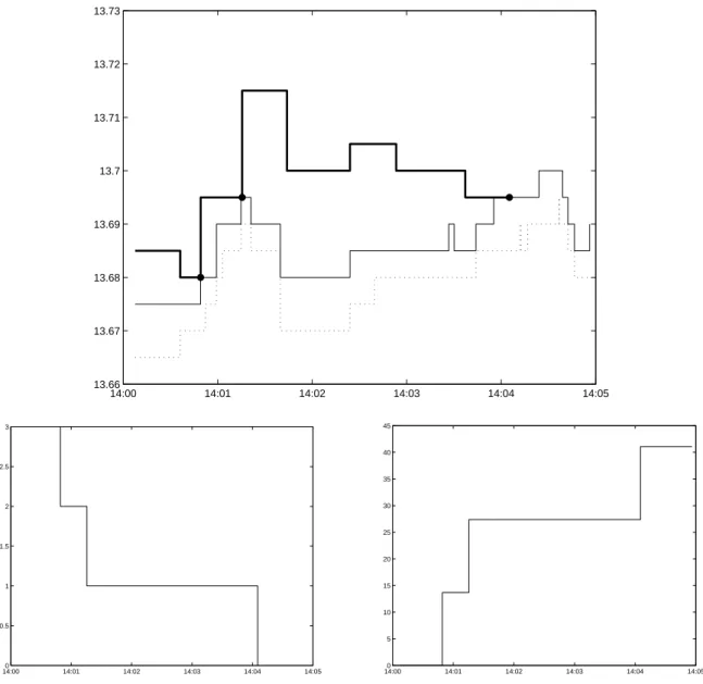
The first two examples (Figures 11 and 12) consist in getting rid of a quantity of shares equal to 3 times the ATS11. The periods have been chosen to capture the behavior in both bullish and bearish markets.
14:00 14:01 14:02 14:03 14:04 14:05 13.66 13.67 13.68 13.69 13.7 13.71 13.72 13.73 14:000 14:01 14:02 14:03 14:04 14:05 0.5 1 1.5 2 2.5 3 14:000 14:01 14:02 14:03 14:04 14:05 5 10 15 20 25 30 35 40 45
Figure 11: Backtest example on AXA (November 5th 2010). The strategy is used with γ = 10 (euro−1) to get rid of a quantity of shares equal to 3 times the ATS within 5 minutes. Top: quotes of the trader (bold line), market best bid and ask quotes (thin lines). Trades are represented by dots. Bottom left: evolution of the inventory. Bottom right: P&L.
10No drift in prices is assumed in the strategy used for backtesting.
11In the backtests we do not deal with quantity and priority issues in the order books and supposed that our
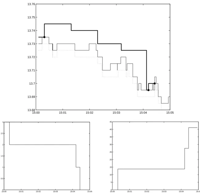
15:00 15:01 15:02 15:03 15:04 15:05 13.68 13.69 13.7 13.71 13.72 13.73 13.74 13.75 13.76 15:000 15:01 15:02 15:03 15:04 15:05 0.5 1 1.5 2 2.5 3 15:000 15:01 15:02 15:03 15:04 15:05 5 10 15 20 25 30 35 40 45
Figure 12: Backtest example on AXA (November 5th 2010). The strategy is used with γ = 10 (euro−1) to get rid of a quantity of shares equal to 3 times the ATS within 5 minutes. Top: quotes of the trader (bold line), market best bid and ask quotes (thin lines). Trades are represented by dots. Bottom left: evolution of the inventory. Bottom right: P&L.
On Figure 11, we see that the first order is executed after 50 seconds. Then, since the trader has only 2 times the ATS left in his inventory, he sends an order at a higher price. Since the market price moves up, the second order is executed in the next 30 seconds, in advance on the average schedule. This is the reason why the trader places a new order far above the best ask. Since this order is not executed within the time window ∆t, it is canceled and new orders are successively inserted with lower prices. The last trade happens less than 1 minute before the end of the period. Overall, on this example, the strategy works far better than a market order (even ignoring execution costs).
On Figure 12, we see the use of the strategy in a bearish period. The first order is executed rapidly and since the market price goes down, the trader’s last orders are only ex-ecuted at the end of the period when prices of orders are lowered substantially since selling becomes of utmost importance. Practically, this obviously raises the question of linking a trend detector to these optimal liquidation algorithms.
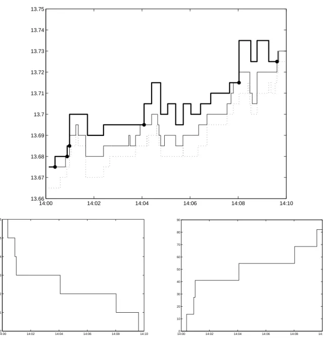
Now, another example is shown on Figure 13 where a trader wants to trade a quantity of shares equal to 6 times the ATS within 10 minutes. The analysis is similar to the preceding ones, the market being even more bullish than in the first example.
14:00 14:02 14:04 14:06 14:08 14:10 13.66 13.67 13.68 13.69 13.7 13.71 13.72 13.73 13.74 13.75 14:000 14:02 14:04 14:06 14:08 14:10 1 2 3 4 5 6 14:000 14:02 14:04 14:06 14:08 14:10 10 20 30 40 50 60 70 80 90
Figure 13: Backtest example on AXA (November 5th 2010). The strategy is used with γ = 10 (euro−1) to get rid of a quantity of shares equal to 6 times the ATS within 10 minutes. Top: quotes of the trader (bold line), market best bid and ask quotes (thin lines). Trades are represented by dots. Bottom left: evolution of the inventory. Bottom right: P&L.
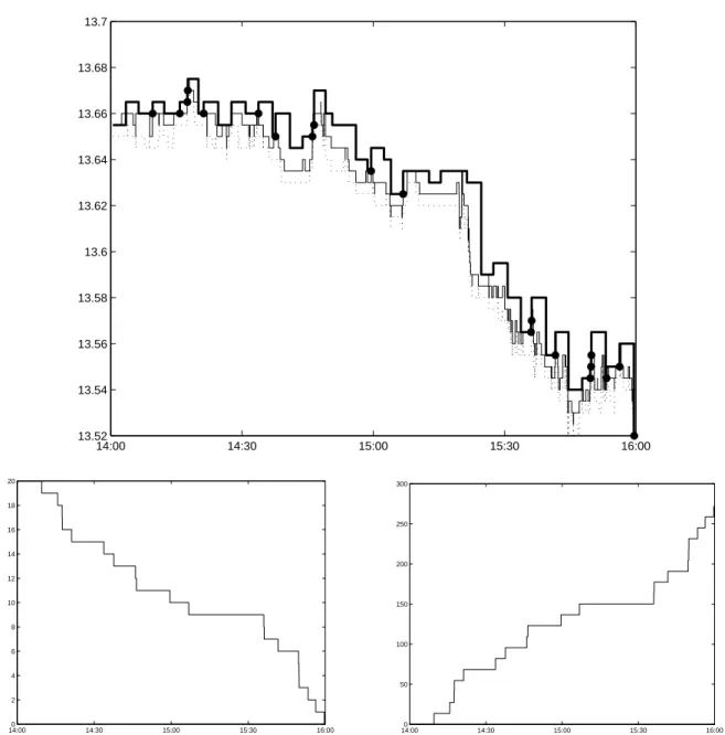
Finally, the model can also be used on longer periods and we exhibit the use of the algorithm on a period of two hours, to sell a quantity of shares equal to 20 times the ATS (Figure 14). 14:00 14:30 15:00 15:30 16:00 13.52 13.54 13.56 13.58 13.6 13.62 13.64 13.66 13.68 13.7 14:000 14:30 15:00 15:30 16:00 2 4 6 8 10 12 14 16 18 20 14:000 14:30 15:00 15:30 16:00 50 100 150 200 250 300
Figure 14: Backtest example on AXA (November 8th 2010). The strategy is used with γ = 1 (euro−1) to get rid of a quantity of shares equal to 20 times the ATS within 2 hours. Top: quotes of the trader (bold line), market best bid and ask quotes (thin lines). Trades are represented by dots. Bottom left: evolution of the inventory. Bottom right: P&L.
Conclusion
As claimed in the introduction, this paper is, to authors’ knowledge, the first proposal to optimize the trade scheduling of large orders with small passive orders. Thanks to an innovative change of variables, it provides an explicit solution in two steps: (1) solve an ODE, (2) deduce the optimal price of the order to be sent to the market.
The choices of modeling made here have been more extensively discussed in [19]. It is nevertheless worthy to underline that no explicit model of what could be called “passive market impact” (i.e. the perturbations of the price formation process by liquidity provision) is used here. Just note that up to now, no quantitative model of this type of impact has been proposed in the literature. Thanks to very promising and recent studies of the multi-dimensional point processes governing the arrival of orders (see for instance the link between the imbalance in the order flow and the moves of the price studied in [11] or [12], or interesting properties of Hawkes-like models in [6]), we can hope for obtaining models of this kind in the near future. The authors will try to embed them into the HJB framework used here. In between, an on-going work dedicated to model dependencies between the Brownian motion supporting St and the Poisson process Nta is under consideration.
Appendix
Proof of Proposition 1:
This is the classical PDE representation of a stochastic control problem with jump pro-cesses.
Proof of Proposition 2 and Theorem 1:
Let’s consider a solution (wq)qof (S) and introduce u(t, x, q, s) = −A−
γq k exp (−γ(x + qs)) wq(t)− γ k. Then: ∂tu + µ∂su + 1 2σ 2∂2 ssu =− γ k ˙ wq(t) wq(t) u− γqµu + γ 2σ2 2 q 2u
Now, concerning the quote, we have: sup sa λ a(sa, s) [u(t, x + sa, q− 1, s) − u(t, x, q, s)] = sup sa Ae −k(sa−s) u(t, x, q, s) [ exp (−γ(sa− s)) ( 1 A wq−1(t) wq(t) )−γ k − 1 ]
The first order condition of this problem corresponds to a maximum (because u is nega-tive) and writes:
(k + γ) exp (−γ(sa∗− s)) ( 1 A wq−1(t) wq(t) )−γ k = k Hence: sa∗− s = 1 kln ( wq(t) wq−1(t) ) + 1 kln(A) + 1 γ ln ( 1 +γ k ) and sup sa λ a(sa, s) [u(t, x + sa, q− 1, s) − u(t, x, q, s)] =− γ k + γA exp(−k(s a∗− s))u(t, x, q, s) =− γ k + γ ( 1 +γ k )−k γ wq−1(t) wq(t) u(t, x, q, s)
Hence, putting the three terms together we get:
∂tu(t, x, q, s) + µ∂su(t, x, q, s) + 1 2σ 2∂2 ssu(t, x, q, s) + sup sa λ a(sa, s) [u(t, x + sa, q− 1, s) − u(t, x, q, s)] =−γ k ˙ wq(t) wq(t) u− γµqu +γ 2σ2 2 q 2u− γ k + γ ( 1 +γ k )−k γ wq−1(t) wq(t) u =−γ k u wq(t) [ ˙ wq(t) + kµqwq(t)− kγσ2 2 q 2w q(t) + ( 1 +γ k )−(1+kγ ) wq−1(t) ] = 0 Now, noticing that the boundary and terminal conditions for wq are consistent with the
Proof of Corollary 1:
The trading intensity associated to the optimal strategy is:
λa∗(t, q) = A exp (−k(sa∗(t, q, s)− s)) = wq−1(t) wq(t) ( 1 +γ k )−k γ
Since the system (S) that defines w is independent of A, the trading intensity is itself independent of A.
Consequently, when optimal strategy is used, the evolution of the inventory, and hence the evolution of the trading curve, does not depend on A.
Proof of Proposition 3:
We have that
∀q ∈ N, ˙wq(t) = (αq2− βq)wq(t)− ηwq−1(t)
Hence if we consider for a given Q ∈ N the vector w(t) = w0(t) w1(t) .. . wQ(t) we have that w′(t) = M w(t) where: M = 0 0 · · · · · · · 0 −η α − β 0 . .. . .. ... 0 . .. . .. ... . .. ... .. . . .. . .. ... . .. ... .. . . .. . .. −η α(Q − 1)2− β(Q − 1) 0 0 · · · · · · 0 −η αQ2− βQ with w(T ) = 1 0 .. . 0
. Hence we know that, if we consider a basis (f0, . . . , fQ) of eigenvectors
(fjbeing associated to the eigenvalue αj2−βj), there exists (c0, . . . , cQ)∈ RQ+1independent
of T such that: w(t) = Q ∑ j=0 cje−(αj 2−βj)(T −t) fj
Consequently, since we assumed that α > β, we have that w∞:= limT→+∞w(0) = c0f0.
Now, w∞ is characterized by:
(αq2− βq)w∞q = ηw∞q−1, q > 0 w0∞= 1 As a consequence we have: w∞q = η q q! q ∏ j=1 1 αj− β
The resulting asymptotic behavior for the optimal ask quote is: lim T→+∞s a∗(0, q, s) = s + 1 kln ( A 1 +γk 1 αq2− βq )
Proof of Proposition 4 and Corollary 2:
To solve the system (S) for σ = 0, we look for a solution of the form wq(t) = h(t)
q
q! . Then, ∀q ∈ N, ˙wq(t) =−βqwq(t)− ηwq−1(t), wq(T ) = 1q=0, w0= 1
⇐⇒ h′(t) =−βh(t) − η h(T ) = 0
Hence, if β = kµ̸= 0, the solution of (S) writes wq(t) = η
q
q!(
exp(β(T−t))−1
β )
q.
From Theorem 1, we obtain the optimal quote:
sa∗(t, q, s) = s + ( 1 kln ( η q exp(β(T − t)) − 1 β ) + 1 kln(A) + 1 γ ln ( 1 +γ k )) Using the expression for η, this can also be written:
sa∗(t, q, s) = s +1 kln ( A 1 +γk 1 q eβ(T−t)− 1 β )
Now, the instantaneous probability of being executed at time t with an inventory q is:
λa∗ = A exp (−k(sa∗− s)) = ( 1 +γ k ) q β eβ(T−t)− 1
Hence, because the intensity is proportional to q, the trading curve t7→ V (t) is charac-terized by the following ODE:
V′(t) =− ( 1 +γ k ) V (t) β eβ(T−t)− 1, V (0) = q0
Solving this equation, we get:
V (t) = q0exp ( −(1 +γ k ) ∫ t 0 β eβ(T−s)− 1ds ) = q0exp ( −(1 +γ k ) ∫ eβT eβ(T−t) 1 ξ(ξ− 1)dξ ) = q0exp ( −(1 +γ k ) [ ln ( 1−1 ξ )]eβT eβ(T−t) ) = q0 ( 1− e−β(T −t) 1− e−βT )1+γk
References
[1] Aur´elien Alfonsi, Antje Fruth, and Alexander Schied. Optimal execution strategies in limit order books with general shape functions. Quantitative Finance, 10(2):143–157, 2010.
[2] R. F. Almgren and N. Chriss. Optimal execution of portfolio transactions. Journal of
Risk, 3(2):5–39, 2000.
[3] Robert Almgren. Optimal Trading in a Dynamic Market. Technical Report 2, 2009. [4] Robert F. Almgren. Optimal execution with nonlinear impact functions and
trading-enhanced risk. Applied Mathematical Finance, 10(1):1–18, 2003.
[5] Marco Avellaneda and Sasha Stoikov. High-frequency trading in a limit order book.
Quantitative Finance, 8(3):217–224, 2008.
[6] E. Bacry, S. Delattre, M. Hoffmann, and J. F. Muzy. Modeling microstructure noise with mutually exciting point processes. January 2011.
[7] Erhan Bayraktar and Michael Ludkovski. Liquidation in Limit Order Books with Con-trolled Intensity. May 2011.
[8] Dimitris Bertsimas and Andrew W. Lo. Optimal control of execution costs. Journal of
Financial Markets, 1(1):1–50, 1998.
[9] Robert J. Bloomfield, Maureen O’Hara, and Gideon Saar. The “Make or Take” Deci-sion in an Electronic Market: Evidence on the Evolution of Liquidity. Social Science
Research Network Working Paper Series, October 2002.
[10] Bruno Bouchard, Ngoc-Minh Dang, and Charles-Albert Lehalle. Optimal control of trading algorithms: a general impulse control approach. SIAM J. Financial
Mathemat-ics, 2011.
[11] Rama Cont and Adrien De Larrard. Price Dynamics in a Markovian Limit Order Book Market. Social Science Research Network Working Paper Series, January 2011. [12] Rama Cont, Arseniy Kukanov, and Sasha Stoikov. The Price Impact of Order Book
Events. Social Science Research Network Working Paper Series, November 2010. [13] Ngoc-Minh Dang. Optimal trading with transient price impact. A comparison of discrete
and continuous approach. Preprint, 2011.
[14] P. A. Forsyth, J. S. Kennedy, S. T. Tse, and H. Windcliff. Optimal Trade Execution: A Mean-Quadratic-Variation Approach, 2009.
[15] Peter A. Forsyth. A Hamilton Jacobi Bellman approach to optimal trade execution.
Applied Numerical Mathematics, October 2010.
[16] Thierry Foucault and Albert J. Menkveld. Competition for Order Flow and Smart Order Routing Systems. October 2006.
[17] Jim Gatheral. No-Dynamic-Arbitrage and Market Impact. Social Science Research
Network Working Paper Series, October 2008.
[18] Jim Gatheral, Alexander Schied, and Alla Slynko. Transient Linear Price Impact and Fredholm Integral Equations. Social Science Research Network Working Paper Series, January 2010.
[19] Olivier Gu´eant, Charles-Albert Lehalle, and Joaquin Fernandez-Tapia. Dealing with the inventory risk. Technical report, 2011.
[20] H. He and H. Mamaysky. Dynamic trading policies with price impact. Journal of
Economic Dynamics and Control, 29(5):891–930, 2005.
[21] Thomas Ho and Hans R. Stoll. Optimal dealer pricing under transactions and return uncertainty. Journal of Financial Economics, 9(1):47–73, March 1981.
[22] G. Huberman and W. Stanzl. Price manipulation and quasi-arbitrage. Econometrica, 72(4):1247–1275, 2004.
[23] Gur Huberman and Werner Stanzl. Optimal Liquidity Trading. Social Science Research
Network Working Paper Series, December 2000.
[24] I. Kharroubi and H. Pham. Optimal portfolio liquidation with execution cost and risk.
Arxiv preprint arXiv:0906.2565, 2009.
[25] Peter Kratz and Torsten Sch¨oneborn. Optimal Liquidation in Dark Pools. Social Science
Research Network Working Paper Series, February 2009.
[26] Charles-Albert Lehalle. Rigorous Strategic Trading: Balanced Portfolio and Mean-Reversion. The Journal of Trading, 4(3):40–46, 2009.
[27] Charles-Albert Lehalle and Romain Burgot. The Established Liquidity Fragmentation Affects all Investors. Technical report, CA Cheuvreux, March 2009.
[28] Charles-Albert Lehalle, Olivier Gu´eant, and Julien Razafinimanana. High Frequency Simulations of an Order Book: a Two-Scales Approach. In F. Abergel, B. K. Chakrabarti, A. Chakraborti, and M. Mitra, editors, Econophysics of Order-Driven
Markets, New Economic Windows. Springer, 2010.
[29] J. Lorenz and R. Almgren. Mean–variance optimal adaptive execution. Applied
Math-ematical Finance, 2011.
[30] Yuriy Nevmyvaka, Michael Kearns, Amy Papandreou, and Katia Sycara. Electronic Trading in Order-Driven Markets: Efficient Execution. E-Commerce Technology, IEEE
International Conference on, 0:190–197, 2005.
[31] Anna Obizhaeva and Jiang Wang. Optimal Trading Strategy and Supply/Demand Dynamics. Social Science Research Network Working Paper Series, February 2005. [32] Gilles Pag`es, Sophie Laruelle, and Charles-Albert Lehalle. Optimal split of orders across
liquidity pools: a stochatic algorithm approach. Technical report, 2009.
[33] S. Predoiu, G. Shaikhet, and S. Shreve. Optimal Execution of a General One-Sided Limit-Order Book. Technical report, Carnegie-Mellon University, September 2010. [34] A. Schied and T. Sch¨oneborn. Risk aversion and the dynamics of optimal liquidation