HAL Id: tel-01398903
https://tel.archives-ouvertes.fr/tel-01398903
Submitted on 18 Nov 2016HAL is a multi-disciplinary open access
archive for the deposit and dissemination of sci-entific research documents, whether they are pub-lished or not. The documents may come from teaching and research institutions in France or abroad, or from public or private research centers.
L’archive ouverte pluridisciplinaire HAL, est destinée au dépôt et à la diffusion de documents scientifiques de niveau recherche, publiés ou non, émanant des établissements d’enseignement et de recherche français ou étrangers, des laboratoires publics ou privés.
et les données synthétiques
Vincenzo Musco
To cite this version:
Vincenzo Musco. Analyse de la propagation basée sur les graphes logiciels et les données synthé-tiques. Ordinateur et société [cs.CY]. Université Charles de Gaulle - Lille III, 2016. Français. �NNT : 2016LIL30053�. �tel-01398903�
Ecole Doctorale des Sciences pour l’Ing´enieur – Lille
TH`
ESE
pour obtenir le grade de
Docteur de l’Universit´
e Lille III
Sp´
ecialit´
e “Informatique”
pr´esent´ee et soutenue publiquement par
Vincenzo Musco
le 3 Novembre 2016Propagation Analysis based on Software
Graphs and Synthetic Data
Directeur de th`ese : Philippe Preux Co-encadrant de th`ese : Martin Monperrus
Jury
Dr. Jean-R´emy Falleri, Universit´e de Bordeaux Rapporteur
Pr. Pascal Poizat, Universit´e Paris Ouest Nanterre la D´efense Rapporteur Pr. Pascale Kuntz-Cosperec, Universit´e de Nantes Examinatrice
Pr. Philippe Preux, Universit´e de Lille Examinateur
Dr. Martin Monperrus, Universit´e de Lille Examinateur
Centre de Recherche en Informatique, Signal et Automatique de Lille (CRIStAL) UMR 9189
iii
Abstract
Programs are everywhere in our daily life: computers and phones but also fridges, planes and so on. The main actor in the process of creating these programs is human beings. As thorough as they can be, humans are known to make involuntary errors without their awareness. Thus, once finished an already hard phase of writing a program, they have to face the maintenance phase on which they have to deal with errors they had previously made. All long their development task, developers have to continuously face their (or their colleagues) errors. This key observation arises the need of aiding developers in their development/maintenance tasks.
Thus, for assisting developers, a large number of tools exist, some still in development, others are integrated in the IDE (debugging, test suites, refactoring, etc.). Some of these tools are manual, while others propose automatic assistance. To be effective, automated tools should capture in the best way as possible how the program is structured and works. For this purpose, one particularly well-suited data structure is graphs, materializing how concepts relate to each other. Using such data structures for proposing assistance tools to developers is a quite promising way to proceed.
In this thesis, we concentrate on tools based on a graph representation of the program. Two big challenges on which we concentrate in this thesis are change impact analysis (CIA) and fault localization (FL). The former concentrates on the determination of the impacts of a potential change which may be issued by the developer while the latter identifies a fault based on what happened during program execution. Both concepts are complementary: the former concentrates on antemortem sight of the problem on which one wants to identify a fault before the failure occurs while the latter concentrates on postmortem sight on which real failures are analyzed to define a way to go back to their sources.
In this thesis, we face two main problems: (i) the lack of a systematic evaluation methodology or framework to assess the performance of change impact analysis techniques and (ii) most current fault localization techniques focus on a specific set of elements reported by their approach without thinking about how they depend on each other across the program as a whole.
In this thesis, we aim at finding solutions to these problems. We present four contri-butions to address the two presented problems. The two first contricontri-butions concentrate mainly on the change impact analysis side of this thesis while the third works on the fault localization side. The last contribution is a possible application for future works. In a few words, this thesis explores the causes and consequences of failures on computer programs by proposing tools based on graphs.
Contents
List of Figures ix List of Tables x List of Algorithms xi 1 Introduction 1 1.1 Context . . . 1 1.2 Problems . . . 2 1.3 Contributions . . . 3 1.4 Outline . . . 5 1.5 Publications . . . 5 1.5.1 Published . . . 5 1.5.2 Under Submission . . . 6 1.5.3 To be Submitted . . . 6 1.6 Reproducible Research . . . 62 State of the Art 7 2.1 Essential Definitions . . . 7
2.1.1 Errors . . . 7
2.1.2 Software Testing and Mutation Testing . . . 8
2.1.2.1 Software Testing . . . 8
2.1.2.2 Mutation Testing . . . 9
2.1.3 Graphs for Software Engineering . . . 10
2.1.3.1 Graph Definition . . . 10
2.1.3.2 Graph Degrees . . . 11
2.1.3.3 Graph Metrics . . . 12
2.1.3.4 Software Graph Granularities . . . 13
2.1.3.5 Software Graph Types . . . 15
2.1.3.6 Static vs. Dynamic Software Graph Extraction . . . 17
2.2 Change Impact Analysis . . . 18
2.2.1 Taxonomy of Change Impact Analysis . . . 18
2.2.2 Terminology of Change Impact Analysis . . . 19
2.2.3 Modern Implementation of Change Impact Analysis . . . 20
2.2.4 Call Graph-based Approaches . . . 21
2.2.5 Other Graph-based Approaches . . . 22
2.2.6 Other Approaches . . . 23
2.2.7 Discussion . . . 24
2.3 Fault Localization . . . 24
2.3.1 Spectrum-based Fault Localization . . . 24
2.3.2 Graph-based Approaches . . . 25
2.3.3 Mutation-based Approaches . . . 26
2.3.4 Discussion . . . 27
2.4 Generative Models of Software Data . . . 27
2.4.1 Generic Generative Models . . . 28
2.4.2 Software Generative Models . . . 28
2.4.3 Discussion . . . 29
3 An Evaluation Framework for Change Impact Analysis 31 3.1 Main Algorithm . . . 33
3.2 Application to Call Graph Based Impact Prediction . . . 34
3.3 Research Questions . . . 37
3.4 Experimental Evaluation . . . 38
3.4.1 Evaluation Protocol . . . 38
3.4.1.1 One-Impact Mutant-Level Accuracy Metrics . . . 38
3.4.1.2 Global Accuracy Metrics . . . 39
3.4.2 Dataset . . . 41
3.4.3 Mutation Operators . . . 41
3.4.4 Empirical Results . . . 42
3.4.5 Discussion . . . 51
3.4.5.1 Other Software Graphs . . . 51
3.4.5.2 Comparison against Impact Prediction Techniques . . . . 52
3.4.5.3 Threats to Validity . . . 52
3.5 Conclusion . . . 53
4 Causal Graph for Change Impact Analysis 55 4.1 Approach Overview . . . 57
4.2 Learning Phase . . . 58
4.2.1 Input Learning Data . . . 58
4.2.2 Computing Weights . . . 58
4.2.2.1 Binary Update Algorithm . . . 59
4.2.2.2 Dichotomic Update Algorithm . . . 59
4.3 Prediction Phase . . . 60
4.4 Research Questions . . . 61
4.5 Experimental Evaluation . . . 61
4.5.1 Evaluation Protocol . . . 61
4.5.1.1 Evaluation and Dataset . . . 62
4.5.1.2 Comparison . . . 63 4.5.2 Empirical Results . . . 63 4.6 Threats to Validity . . . 69 4.6.1 Internal Validity . . . 69 4.6.2 Construct Validity . . . 69 4.6.3 External Validity . . . 69 4.7 Conclusion . . . 69
5 Causal Graph for Fault Localization 71 5.1 Technical Contribution . . . 73
5.1.1 Intuition . . . 73
Contents vii 5.2 Research Questions . . . 75 5.3 Experimental Evaluation . . . 76 5.3.1 Evaluation Protocol . . . 76 5.3.1.1 Evaluation Metrics . . . 76 5.3.1.2 Comparison . . . 77 5.3.1.3 Dataset . . . 78 5.3.1.4 Mutation Operators . . . 79 5.3.2 Empirical Results . . . 80 5.4 Threats to Validity . . . 85 5.5 Conclusion . . . 86
6 Generation of Synthetic Software Dependency Graphs 87 6.1 Common Structure of Dependency Graphs . . . 89
6.1.1 Protocol . . . 89
6.1.1.1 Dependency Graph Extraction . . . 89
6.1.1.2 Dataset . . . 90
6.1.1.3 Comparison of Degree Distributions . . . 90
6.1.2 Results . . . 91
6.1.3 Summary . . . 92
6.2 A Generative Model for Dependency Graphs . . . 93
6.2.1 Assumptions . . . 93
6.2.2 The Generalized Double GNC Algorithm (GD-GNC) . . . 93
6.2.2.1 Relation to Assumption #1 and #2 . . . 94
6.2.2.2 Relation to Assumption #3 . . . 95 6.2.2.3 Analysis . . . 95 6.2.2.4 Parameters . . . 96 6.3 Experimental Evaluation . . . 96 6.3.1 Comparison . . . 96 6.3.2 Protocol . . . 97 6.3.2.1 Error metric . . . 97 6.3.2.2 Parameter Optimization . . . 98 6.3.3 Results . . . 98 6.3.4 Scalar Properties . . . 100 6.4 Discussion . . . 100 6.4.1 Threats to Validity . . . 101 6.4.2 Practical Implications . . . 101 6.5 Conclusion . . . 101 7 Conclusion 103 7.1 Summary . . . 103 7.2 Perspectives . . . 104
7.2.1 Better Propagation Profiles . . . 104
7.2.2 Faster Computation of Propagation Profiles . . . 105
7.2.3 Other Types of Software Graphs . . . 105
7.2.4 Propagation Profiles at Other Granularities . . . 105
7.2.5 Alternative Evaluation of Generative Models . . . 106
A Reproducible Research 107
C Generative Model – Other directions 111 C.1 Generic Graphs . . . 111 C.2 Different Versions . . . 112
List of Figures
1.1 Problems and contributions of this thesis . . . 3
2.1 Error terminology . . . 8
2.2 Illustration of software testing and mutation testing . . . 9
2.3 Illustration of a directed and an undirected graph . . . 11
2.4 In-edges and out-edges for a simple digraph example . . . 12
2.5 Cumulative degree distribution function . . . 13
2.6 Example of a path of length 2 and triangles . . . 14
2.7 Software Granularities . . . 15
2.8 Illustration of endo- and exo-dependencies . . . 16
2.9 Illustration of Bohner’s sets . . . 19
2.10 An example of the FindCallers feature in IntelliJ IDEA 2016.1 . . . 21
3.1 Visualization of the effect of a particular mutation . . . 35
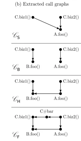
3.2 Four types of call graphs . . . 36
3.3 Example of a call graph in which a change has been introduced . . . 37
3.4 Number of impacted nodes for ABS mutants for each project . . . 51
4.1 Strogoff’s technique based on weighted call graphs . . . 58
4.2 K-fold cross validation . . . 62
4.3 Performances improvement of Dichotomic over FindCallers . . . 65
4.4 Impact of the prediction threshold on the F -score . . . . 66
4.5 Weights learned using Binary and Dichotomic . . . 67
5.1 Example of causal graph extraction . . . 73
6.1 Degree distribution for exo- and endo-dependencies . . . 89
6.2 In- and out-degree distribution for 50 programs . . . 92
6.3 GNC-Attach: the GNC primitive operation . . . 94
6.4 Influence of the GNC-Attach primitive . . . 96
6.5 Influence of p on the GD-GNC algorithm . . . . 97
B.1 Impact of the prediction threshold on the F -score . . . 109
C.1 Inverse cumulative degree distributions for various generative models . . . 112
C.2 Obtained generations from scratch and from an older version . . . 113
3.1 Four types of call graphs for impact prediction . . . 34
3.2 Statistics about the projects considered in this chapter . . . 40
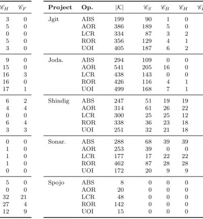
3.3 Statistics about generated call graphs . . . 42
3.4 Mutation operators . . . 43
3.5 Mutation statistics based on four different call graphs . . . 44
3.6 Proportion of predictions in pS and pC sets . . . 45
3.7 Main metrics of impact prediction based on call graphs . . . 46
3.8 Main computation times . . . 49
4.1 Comparative effectiveness for predicting sensitive call sites using Strogoff . . . 64
4.2 Execution time of Strogoff . . . 68
5.1 Descriptive statistics of the fault dataset . . . 79
5.2 Average wasted effort in number of inspected methods . . . 80
5.3 Number of perfect predictions . . . 81
5.4 Times required for each step of Vautrin . . . 83
6.1 The 50 Java programs considered in this chapter . . . 91
6.2 Number of times the H0 hypothesis is rejected . . . 93
6.3 Best parameters for Baxter and GD-GNC . . . 98
6.4 Metrics computed for GD-GNC and Baxter & Frean models . . . 99
List of Algorithms
3.1 Computation of the candidate and actual impact sets . . . 33
3.2 Computation of the Bohner’s set . . . 40
4.1 Call graph weight learning algorithm . . . 59
4.2 Algorithm Binary . . . 59
4.3 Algorithm Dichotomic . . . 60
4.4 Impact prediction algorithm based on a causal graph . . . 60
5.1 Vautrin’s prediction algorithm . . . 75
6.1 GNC-Attach Algorithm . . . 94
6.2 Iterative algorithm for the GD-GNC generative model . . . 95
1
Introduction
‘ ‘Anyone who has never made a mistake has never tried anything new.” — Albert Einstein
1.1
Context
Our today’s life is surrounded by machines. A large range of our daily tasks are ensured by computer systems. In order to be able to accomplish anything, computer systems require that each task be clearly defined. This is achieved by the means of computer programs. Developers are the key people who are responsible for creating these programs by writing source code in a way the computer is able to understand.
Unfortunately, developers are humans, and humans are well-known to make mistakes. There is no exception for computer programs: as they are written by humans, they are error-prone. These errors, embedded in the software source code, are a part of the running logic and lead to various undesired run-time behaviors: unexpected program terminations, unresponsive UI components (such as buttons, menu item, etc.), or even system crashes. Debugging tasks can quickly become a brain-teaser for the developer as source code can be made of thousands of lines of code, split in hundreds of files. As a consequence, the number of possible source code locations for a fault can be very high. Moreover, some errors may not be detected by the compiler and remain silent until the program is executed: an example of such an error is a null pointer exception which is caused by calling a method on an object variable which in fact contains a null value.
Furthermore, when a code change is introduced in a program, it can have side effects. Indeed, a developer can introduce a change C1 in his source code which make another
piece of source code somewhere else in the program defective. These side effects can appear in a totally different point than where the original changes have been made. At the same time, when a developer or a software tester identifies an undesired behavior in the program, the obvious task is to correct the source code in order to make it work correctly. However, the precondition is to locate the fault in the source code: this step may be harder to achieve than fixing the problem itself. For instance, a developer working on a calculator application may change arithmetic-related code, e.g., division function. Then, when running the program, the user interface buttons of the calculator may not respond anymore. At first sight, the developer may think the button source code is defective while the root cause may be the arithmetic-related change.
Towards the omnipresence of these faults and the difficulty to locate them, a large range of approaches have been proposed to assist in debugging and fixing tasks. It begins early in the development stage with the software documentation: the developer adds comments his source code. They are neither compiled nor executed lines of code which help the developer to remember what he has done. Moreover, using an efficient logging system can help the developer as well as anyone else working on the code to identify where he should search and fix the source code.
Software testing is a popular approach in which the developer writes simple use cases of his code which will be run again and again during the development phase to ensure that any fault has been introduced in previously developed code.
Bug report systems and issue tracking systems propose to other people to report and discuss failures they face with a program. Thanks to Version Control Systems (a.k.a. VCS), such as Git or Subversion, developers can easily collaborate on projects and benefit from useful features such as source code versioning, i.e., tracing the history of program changes back.
A large number of techniques have been proposed by the software engineering research community for assisting developers when facing faults. These techniques are intended to help developers in detecting, locating and even fixing faults. Some tools are not only related to faults, but are also intended for assisting the developers with numerous tasks which may be tedious to handle manually and which may even lead to new faults. As an example, refactoring proposes to automatically handle moving pieces of code, renaming methods and so on, while ensuring the program coherence.
These approaches generally use any software artifacts to achieve their purpose. These artifacts include the source code itself, but also everything previously cited: documenta-tion, bug reports, software testing, version control systems informadocumenta-tion, etc. For instance, in this thesis, we use the program source code to produce graphs (presented in Sec-tion 2.1.3) which expose the links between different program parts, and the program tests as a way to observe the program failures. These pieces of information are used for change impact analysis (presented in Section 2.2) on which we want to estimate the impacted tests based on a specific change and fault localization (presented in Section 2.3) on which we determine a fault in the code based on a set of failing tests.
In conclusion, detecting, locating and fixing program faults is time-demanding, tedious and difficult. Any change can break other program parts. For this reason, many tools are proposed to assist developers in their daily tasks. As time goes by, systems are becoming more and more complex, this assistance will thus be more and more appreciated.
1.2
Problems
In this thesis, we concentrate on problems related to propagation analysis. Propagation analysis consists in analyzing how a change inserted somewhere in the source code spreads through the software method callers, dependent variables and fields, etc. in such a way that it will have influence in other parts of the program. An obvious example is a failure due to the propagation of a fault inserted somewhere in the program.
In this failure perspective, the propagation problem can be seen from two points of view: antemortem and postmortem propagation. Antemortem propagation consists in reporting possible impacts of a change (i.e., a fault) to the developer while he is typing it down on his source code editor, without requiring to run the code to notice the impacts (i.e., a failure). Analyzing the propagation in this way is known as change impact analysis (CIA).
1.3. Contributions 3
Figure 1.1: Problems and contributions of this thesis.
Problem 1
For existing change impact analysis techniques, there is no systematic evaluation methodology or framework to assess their performances. The performance is defined by the ability to locate elements really impacted by a change.
Postmortem propagation consists in reporting a set of elements (i.e., potential faults) which are responsible of a specific impact (i.e., program or system failure). In this ap-proach, the fault detection is done once the failure occurs, that is, once the developer runs his code. Analyzing the propagation in this way is known as fault localization. In essence, the fault localization process tries to capture causality relationships between code elements.
Problem 2
Most current fault localization techniques do not consider the whole program, they focus on a specific set of elements reported by their approach without thinking to how they depend on each other across the program as a whole.
In this thesis, we tackle these problems based on two intuitions. The first intuition is that software graphs are data structures materializing how code elements are intercon-nected. They offer a global vision of the interactions between the different concepts they materialize. Thus, they are a good candidate for exploring propagation and its inherent causality. The second intuition is that synthetic data are good candidates for simulating hard-to-obtain software information such as atomic software changes. In change impact analysis and fault localization, software mutants can be used as synthetic faults.
1.3
Contributions
The contributions of this thesis are answers to problems presented in Section 1.2. Fig-ure 1.1 is a simplified representation of how these problems and the contributions proposed in this thesis are articulated. As we can see, the source code can be used for three different purposes:
1. producing a call graph; 2. generating software mutants;
3. deriving some properties to feed a graph generator.
Based on these graphs and mutants, we propose four contributions that are presented in the remaining of this section. On the first three contributions, we extensively rely on program test suites: we consider them as an accurate way to observe impacts on a program. Thus, these contributions work at the method level.
Two contributions are related to change impact analysis, i.e., determinate potential impacts (failures) related to a change (faults).
Contribution 1
An evaluation framework for assessing the performance of a change impact analysis technique inspired from mutation testing.
The first contribution addresses the first problem. This framework is based on syn-thetic seeded faults obtained using mutation testing. The performances are assessed based on the program test execution result, i.e., the ability of the change impact analysis tech-nique to report the tests which actually fail on run-time. Any change impact analysis technique would be assessable using this framework. We evaluate impact prediction of four types of call graphs. This evaluation enables us to study how the error propagates and is based on 16,922 mutants created from 10 open-source Java projects using 5 classic mutation operators.
Contribution 2
A novel change impact analysis technique based on information learned from past impacts and call graph.
The second contribution is a novel call graph-based change impact analysis approach. We use software mutants and their execution profile to learn causes of failures on the call graph resulting in a new type of graph, the causal graph. We evaluate our system using our evaluation framework (Contribution 1) and considering 9 open-source Java projects totaling 450,000+ lines of code. We simulate 16,682 changes and their actual impact through code mutations, as done in mutation testing.
Contribution 3
A new fault localization algorithm, built on an approximation of causality based on call graphs.
The third contribution makes use of graphs and mutants to evaluate their potential for fault localization, i.e., determinate causes (faults) of specific impacts (failures). We propose to use similar causal graphs as these used in Contribution 2. They are used to assist popular fault localization techniques in order to improve their performance. We evaluate our approach on the fault localization benchmark of Steimann et al. totaling 5,836 faults. This third contribution addresses the second problem.
Contribution 4
1.4. Outline 5
As we extensively work with synthetic faults, i.e., software mutants, we want to push further the experiments in generating software graphs for propagation analysis. Our last contribution is the first step toward this goal: we propose a new generative model of synthetic software dependency graphs. This model is used to generate synthetic graphs aiming at being similar to real ones. We extract the dependency graph of 50 open-source Java projects, totaling 23,178 nodes and 108,404 edges that we compare to generated graphs for assessing their fitness.
To sum up, we propose in this thesis four contributions for software engineering as-sistance. Two are used in the improvement of change impact analysis, one for fault localization and the last is a first step for future research.
1.4
Outline
The remaining of this thesis is structured as follows. In Chapter 2, we present the con-cepts as well as the works related to this thesis. In Chapter 3, we present our evalua-tion framework for change impact analysis and assess it with four flavors of call graphs (Contribution 1). In Chapter 4, we propose to use a learning technique to improve call graph-based change impact analysis (Contribution 2). In Chapter 5, we present a call graph-based fault localization technique used to improve the state-of-the-art ones (Con-tribution 3). In Chapter 6, we present our generative model for software dependency graphs (Contribution 4). In Chapter 7, we conclude this thesis and present perspectives.
1.5
Publications
In this section, we present the publications related to contributions presented in Sec-tion 1.3.
1.5.1
Published
[1] Vincenzo Musco, Antonin Carette, Martin Monperrus, and Philippe Preux. A Learn-ing Algorithm for Change Impact Prediction. In ProceedLearn-ings of the 5th International Workshop on Realizing Artificial Intelligence Synergies in Software Engineering co-located with ICSE, RAISE ’16, pages 8–14, 2016.
[2] Vincenzo Musco, Martin Monperrus, and Philippe Preux. An Experimental Protocol for Analyzing the Accuracy of Software Error Impact Analysis. In Proceedings of the 10th International Workshop on Automation of Software Test co-located with ICSE, AST ’15, pages 60–64, 2015.
[3] Vincenzo Musco, Martin Monperrus, and Philippe Preux. A Large-scale Study of Call Graph-based Impact Prediction using Mutation Testing. Software Quality Journal, 2016. To appear.
[4] Vincenzo Musco, Martin Monperrus, and Philippe Preux. Mutation-based graph in-ference for fault localization. In Proceedings of the International Working Conin-ference on Source Code Analysis and Manipulation, October 2016.
Publications [2, 3] covers contribution 1, publication [1] covers contribution 2 and pub-lication [4] covers contribution 3.
1.5.2
Under Submission
[1] Vincenzo Musco, Martin Monperrus, and Philippe Preux. A Generative Model of Software Dependency Graphs to Better Understand Software Evolution. Journal of Software: Evolution and Process, 2016. Minor Revision.
Publication [1] covers contribution 4.
1.5.3
To be Submitted
[1] Vincenzo Musco, Martin Monperrus, and Philippe Preux. Strogoff: A Recommenda-tion System for Finding Sensitive Method Callers with Weighted Call Graphs.
Publication [1] covers contribution 2.
1.6
Reproducible Research
Many existing publications lack public implementations and, as a consequence, are hardly reproducible. As we opted for open-science, all our source code and dataset used to run our experiments are freely available online. For more information, please refer to Appendix A.
2
State of the Art
‘ ‘Smart people learn from their mistakes. But the real sharp ones learn from the mistakes of others”
— Brandon Mull , Fablehaven
In this chapter, works related to this thesis are presented. This chapter is split in four parts. Section 2.1 presents essential definitions and concepts used in this thesis. Then, in the three following sections, we present related works. Section 2.2 covers change impact analysis related to contributions 1 and 2. Section 2.3 covers fault localization related to contributions 3 and Section 2.4 covers generative graph models for software engineering related to contributions 4.
2.1
Essential Definitions
In this section, we present fundamental yet essential concepts of software engineering used in this manuscript.
2.1.1
Errors
This manuscript deals with the detection of errors in programs. We present here a termi-nology used in software engineering based on the error stage.
Many terms are used to refer to software errors and even if they are frequently used interchangeably, they have not exactly the same meaning. To avoid confusion, in this manuscript, we use exclusively the terms fault, error and failure presented by Avizienis et al. [14] defined as:
Fault the physical presence in source code of elements which do not comply with the software specification and can lead to future program malfunctions;
Error the state of a program once a fault has been activated, i.e., the fault code has been run by the system and has started altering the correct state of the system. At this step, the system may continue to run without concrete observable malfunctions; Failure a program which has deviated from the expected behavior. When a failure
oc-curs, the expected behavior is not anymore respected, resulting in noticeable conse-quences such as unexpected program terminations due to a null pointer exception.
Figure 2.1: In the development phase, the fault occurs in the source code. In the running phase, the error is present in the system memory and the failure is the manifestation of a fault
A failure can go beyond the scope of the program and reach the whole system, e.g., resulting in kernel crashes observable with the infamous BSOD1 in Microsoft operating systems.
Figure 2.1 illustrates these concepts. As we can see, faults occur in the development phase, while errors and failures occur during the running phase.
2.1.2
Software Testing and Mutation Testing
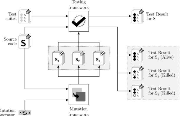
Contribution 1, 2 and 3 presented in Section 1.3 mainly rely on software testing and mutation testing concepts. In this Section, we briefly present these concepts. Mutation testing is based on software testing as shown in Figure 2.2 which illustrates them.
2.1.2.1 Software Testing
When a developer decides to change some parts of his software code, he cannot directly estimate the impacts of his change. Generally, a developer has a rough estimation of these impacts, however, effects beyond his estimations may be possible.
The main goal of software testing [115] is to develop special content along with the source code which will be used to ensure the software execution does not deviate from its expected behavior.
Software testing is defined using test suites, which are classes grouping test cases related to similar software functionalities. Test cases are used to describe the expected behavior based on three components:
1. a set of input data used for testing. These can be of different nature: parameters, fields, global variables, etc.;
2. a test scenario describing the computation to perform on the input data and the values to return;
3. a test oracle determining if the returned values are acceptable or not. In other terms, it determines if the test should pass (i.e., succeed) or fail.
In this way, the developer can ensure his changes have not broken the initial logic by running the test suite of the program. If all tests pass, this indicates that the execution
2.1. Essential Definitions 9
Figure 2.2: Illustration of software testing and mutation testing. Produced (three) mu-tants are in the gray dashed box. Test execution for mumu-tants is in the gray dotted box. Passing tests are black, failing are white ones.
logic remains unchanged for other software parts. However, if at least one test fails, it means the change has an impact somewhere in the program. As a consequence, the developer will have to check his code to fix the problem.
In order to be useful, software testing requires that the test suite be well-designed. A good testing design requires that each piece of code have a test which is related to it in a way to ensure a good code coverage. The code coverage describes the proportion of statements which is covered (i.e., executed) by the tests. A high coverage means that tests run a large number of statements (e.g., each branch of a if-statement, each methods). A poor code coverage implies that test suite does not run a large number of code statements. Figure 2.2 illustrates the testing process (as well as mutation process presented in the next section). As we can see, the testing framework takes as input test suites and the source code (S) and produces test results (for S, the first result has to be considered). In this example, we can see a test suite made of three test cases. All three test pass (black circle).
2.1.2.2 Mutation Testing
Mutation testing [32, 3, 33] is an approach intended to improve the code coverage of test suites. This approach is based on creating several copies of a program, called mutants, in which one (or several) small change(s) is (are) introduced.
By running test suites on each mutant, these are used to exhibit source code parts which require more testing. Indeed, each time we change a part of the code (i.e., we mutate the code), we introduce a little fault which should be detected by our test suites. If the change is not detected, it indicates that the change is not properly covered by test suites.
said to be alive and implies the test coverage could be improved. In the opposite case, if at least one test fails, the mutant is said to be killed and implies that the test covers the part which has been mutated.
The type and the way elements are changed is defined by a mutation operator. Thus, a mutation operator defines:
1. the domain in which code elements should be included in order to be a candidate for mutation;
2. the logic used to concretely achieve the mutation.
As an example, let us consider an arithmetic mutation operator. Its domain includes binary operations which involve an arithmetic operator such as +, -, * and / between the left and right operand. The mutation logic is to replace the arithmetic operator by any other one. Thus, the 1 == 2 expression is not included in the domain and cannot be mutated using this mutation operator. On the other side, the expression 1 + 2 belongs to the domain, its mutation will result in expressions such as 1 - 2, 1 * 2 and 1 / 2.
Figure 2.2 illustrates the mutation testing process. As we can see, the mutation framework takes as input a mutation operator and a source code (S). It produces some mutants (in this example, three mutants are produced: S1, S2 and S3 in the gray dashed
box). Then, we feed these mutants to the testing framework (one at a time) as well as the test suites to obtain test results. In this example, results related to our mutants are ones in the gray dotted box. We can see that, for S1, all test pass (black circles), which
means that S1 is an alive mutant. For S2 and S3, we see that there is one failing test in
each (white circle) which means that these mutants are killed.
More information about research in mutation testing is presented in the survey pro-posed by Jia and Harman [72].
2.1.3
Graphs for Software Engineering
As presented in Section 1, our first intuition is that graphs are good candidates to explore propagation. In this section, we present graphs and all concepts related to graphs which are of interest in the scope of this manuscript. Curious readers interested in graph theory can read good references in the domain among [57, 28, 27, 157, 53, 120].
2.1.3.1 Graph Definition
A graph, also known as network, is a mathematical tool used to model a large number of problems which involve concepts and connections between these. A graph G is made of two sets: a set of nodes N (also called vertices) defining concepts and a set of edges E describing the connections between concepts. An example of such a graph is the connec-tion of peripherals in a network where nodes are network devices (e.g., computer, router) and edges are added between two peripherals every time they are physically or logically connected together. A formal definition of a graph is given by Equation (2.1).
G = {N, E} (2.1)
Where the edges E can be defined using a pair given in Equation (2.2).
E = (n1, n2) (2.2)
2.1. Essential Definitions 11
(a) Computer Network (b) Trophic Network
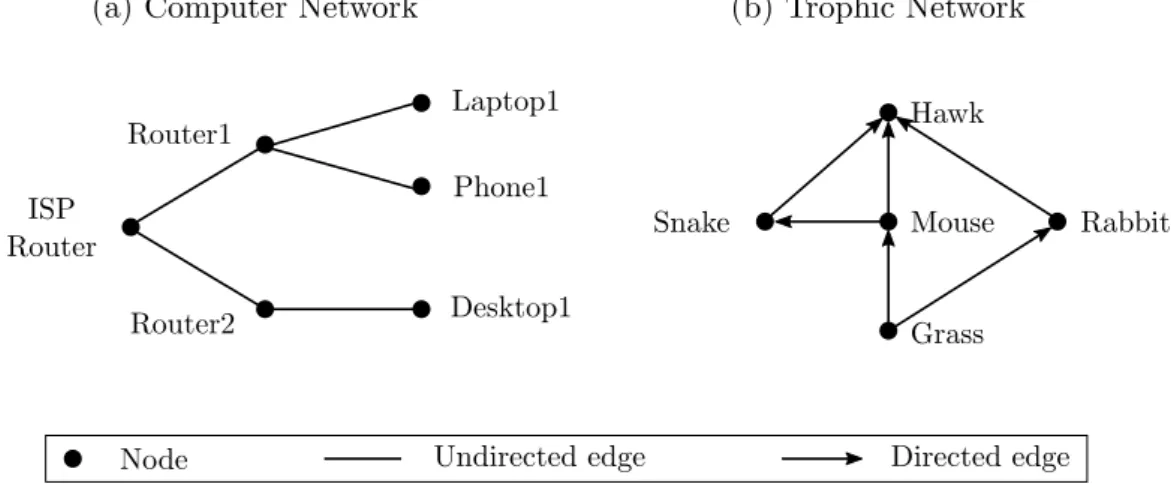
Figure 2.3: (a) illustrates a computer network graph made of 6 nodes and 5 edges. As the communication is bidirectional they can be undirected. (b) shows a trophic network made of 5 nodes and 6 edges. As the concept of “who eats who” is important, they must be directed.
A graph can be either undirected or directed : in the former, edges direction is not taken into consideration while it is in the latter. Directed graphs are also named digraphs. The usage of direction is defined by the modeled concept.
Figure 2.3 gives an example of each type of graph. Figure 2.3a illustrates a network example: an undirected graph is used as peripherals communicate in both directions (i.e., if two peripherals are physically or logically connected together, they can both communi-cate with each other). Figure 2.3b shows an example of directed graph: the predator-prey graph models how an organism eats another. Indeed, there is a relation between the hawk and the rabbit as the former eats the latter. But this observation is valid in one direction only: the rabbit does not eat the hawk.
Equation (2.2) is used to express both directed and undirected edge. In the former, this pair is ordered as the order expresses the direction of the relationship. Thus, Equa-tion (2.2) expresses a directed edge going from n1 to n2 such as n1 −→ n2. In the latter,
the pair is not ordered as the direction is not important.
A large amount of information can be embedded in nodes and edges. This can be labels (e.g., the IP address of a peripheral, an organism class), weights or any other type of data.
A path is an ordered list of nodes for which each pair of nodes in the list is connected by an edge in the graph. The path length is the number of pairs in this list. and the shortest path between two pairs of node is the path with the smallest length among all possible paths between these two nodes.
In this thesis, we distinguish two types of graphs: these resulting from an analysis of software systems and these created by a generative model. The former are qualified as “empirical” or “true”, the latter being qualified as “synthetic” or “artificial”.
2.1.3.2 Graph Degrees
The in-degree and the out-degree of a node n1are respectively the number of edges going to
n1 (i.e., the number of edges (·, n1)) and the number of edges leaving n1 (i.e., the number
of edges (n1, ·)). We use the term degree to refer to both of these concepts and terms
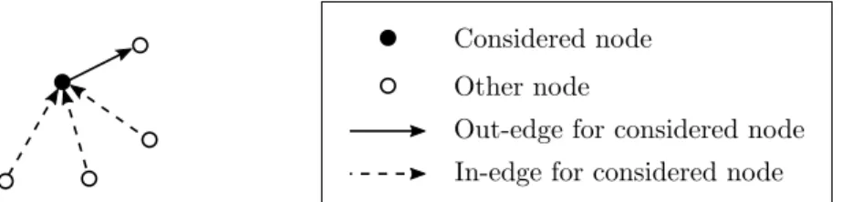
Figure 2.4: In-edges and out-edges for a simple digraph example.
do not exist for undirected graphs. Figure 2.4 illustrates a graph made of 4 nodes. Let us consider the black node, it contains three entering edges (dashed ones) and one leaving edge (plain one). Thus, as a consequence, the in-degree of this node is 3, its out-degree is 1 and its general degree is 3 + 1 = 4.
The degree distribution of a graph is the proportion of each degree in this graph. The total of these proportions sums to 1. In this thesis, we consider cumulative distribution functions (CDF) of degrees which express the proportion of nodes whose degree is smaller or equal to a given value. The main reason is that noncumulative distributions are to be avoided as they are sources of mistakes [91]. Cumulative distributions are more ap-propriate to analyze noisy and right-skewed distributions [119]. The inverse cumulative distribution functions of degrees (ICDF) is the inverse of the cumulative distribution, i.e., the proportion of nodes whose degree is greater or equal to a given value k as expressed by Equation (2.3) where n is the number of nodes in the graph.
ICDF (k) = n − CDF (k − 1) (2.3)
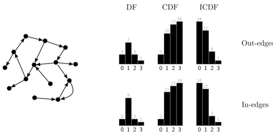
Figure 2.5 illustrates these concepts for a simple digraph made of 14 nodes and 16 edges. Upper histograms illustrate the out-degree functions and the lower ones illustrate the in-degree functions. Leftmost histograms illustrate degree function (DF), central ones illustrate the cumulative degree function (CDF) and the rightmost illustrates the inverse cumulative degree function (ICDF). The small gray number of nodes on top of each bar reports the number for considered degree. Thus, considering in-edges, we can observe that there are 2 nodes with no in-edge and 9 nodes with in-degree 1. Now, if we consider the CDF for in-edges, we observe that there are 11 nodes which have an in-degree lower or equal to 1. For the ICDF, there are 12 nodes which have an in-degree higher or equal to 1.
2.1.3.3 Graph Metrics
There are a host of properties that describe various aspects of a graph, the relation between these properties being more or less understood. Let us mention the properties we consider in this manuscript:
Density the graph density expresses the proportion of pairs of nodes being connected in the graph. The graph density is computed using formula (2.4);
δ = |E|
|N | × (|N | − 1) (2.4)
Diameter the length of the longest shortest path between any pair of nodes;
Average shortest path length the average length of the shortest path between any pair of nodes;
2.1. Essential Definitions 13
Figure 2.5: An example of directed graph with its corresponding in- and out-degree func-tion (DF), cumulative degree funcfunc-tion (CDF) and inverse cumulative degree funcfunc-tion (ICDF).
Transitivity (a.k.a. clustering coefficient) indicates how elements are connected to each other. It is defined by the number of triangles divided by the number of paths of length 2 found in the graph. We define a path of length two as two edges between three nodes n1, n2 and n3 such as n1 is connected to n2 and n2 is connected to n3.
A triangle is a closed path of length 2 such as on the previous example, there is a third edge connecting n3 to n1. Figure 2.6 illustrates these concepts, Equation (2.5)
shows a formal definition of the transitivity C;
C = number of triangles
number of paths of length 2 (2.5)
Modularity is a metric used to define how nodes groups are split in modules. A module is defined as a subset of nodes which have a dense connection between them (i.e., contain more edges between them) than with the other nodes of the graph.
The transitivity and the modularity are two different measures of whether there exist some subsets of nodes which are more connected to each other than the average. Though the exact relation between these two metrics is not yet clear, there are some similarities [123].
2.1.3.4 Software Graph Granularities
Granularity is defined by the Oxford dictionary as “the scale or level of detail present in a set of data or other phenomenon”. When working with software data, this granularity concept is central and should be taken into consideration depending on what phenomenon we want to study.
At coarser granularities, we consider more global concepts while finer ones allow to deal with more detailed concepts. As an example, in Java programming language, packages are more global than classes. Classes are grouped in packages, thus working at the package granularity would imply that many classes are “hidden” behind a specific package.
Coarser granularities result in a smaller amount of data, offering the advantage of being easy to manipulate, but the drawback is offering a poor precision because finer concepts are hidden behind coarser ones. At the opposite, a finer granularity proposes to
Figure 2.6: Example of a path of lenth 2 (solid lines) and a triangle (solid and dashed lines together).
obtain a larger amount of data which offers a better precision, but requires more resources and time to process as the amount of data can be very important.
Considering the graph perspective, as graphs can illustrate the interconnection of software concepts, they potentially can materialize concepts of any granularities (some authors also mix concepts from several granularities [49, 128]).
Figure 2.7 illustrates some granularities existing in software engineering and more specifically in Java object-oriented programming language. We observe the following granularities (from coarser to finer):
1. system: interactions between machines;
2. software: interaction of programs and libraries in the system itself;
3. package: group of classes generally intended to achieve same type functionalities; 4. class: concepts containing methods and fields which are intended to be initialized
as an object by the mean of a constructor;
5. feature: one service proposed by a class and its internal state, i.e., methods and fields;
6. (basic) block: a set of consecutive program instructions which contains one entry point;
7. instruction: one command in a source code;
8. token: one item which assembled with other tokens forms instructions.
These are vertical granularities as they can be seen as a Russian nesting doll where each upper level is a generalization of the lower one. Note that as presented previously, coarser granularities indicate a poor precision than finer ones, but in some cases, a coarser granularity is required to analyze some concepts. As an example, in order to study interconnections of systems in a network, considering finer granularities is meaningless.
Horizontal granularity defines for each vertical granularity, how many different types of information can be embedded. Examples of horizontal granularities are:
• at the system vertical granularity: standalone applications, system libraries, user libraries, etc.;
• at the feature vertical granularity: methods, fields, inheritance information, etc. When working at the software vertical granularity, data can be split in two types: ap-plication and library data. Apap-plication data belongs to core software itself. Library data belongs to an external library or programs called by the core program.
2.1. Essential Definitions 15
Figure 2.7: Software granularities for Java programming language (not exhaustive).
For instance, in a software graph, application nodes are related to core program con-cepts while library nodes are related to external library ones. Thus, if the graph is based on a Java program, a class of the software package “Eclipse” may use a class in java.util library. The former is an application node, the latter is a library node.
As a consequence, two types of edges exist:
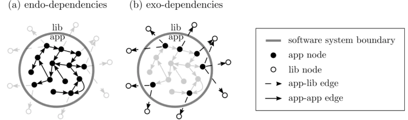
• app-app edges application nodes to application nodes, we call them endo-dependencies, they express that a core element depends on another core element;
• app-lib edges application nodes to library nodes, we call them exo-dependencies, they express that a core element depends on a library element.
For example, if a software method calls the System.out.println method, it is an exo-dependency as this method is member of the Java standard library. Exo-dependencies can occur at each granularity level, even if in lower ones, it is less meaningful to take this concept into consideration.
Figure 2.8a emphasizes endo-dependencies and Figure 2.8b shows exo-dependencies with dashed arrows crossing the system boundary.
2.1.3.5 Software Graph Types
A large number of graphs can be obtained from a program, each one focusing on par-ticular characteristics. Hence, nodes and edges can have various meanings. A common observation is that software graphs are generally directed.
In the remaining of this section, we present some of the most common software graphs. However, this list is far from being exhaustive. We present here only graphs which are
(a) endo-dependencies (b) exo-dependencies
Figure 2.8: Illustration of the set of (a) endo-dependencies and (b) exo-dependencies in a dependency graph.
produced from the program source code. Other types of graphs exist (such as the col-laboration graph materializing relations between developers and the source code) but are out of the scope of this thesis.
Dependency Graph a high-level graph materializing the dependence relationship exist-ing between modules of same nature (e.g., packages, classes). A concept A depends on a concept B if A makes any type of usage of B. Thus, in this graph, nodes are modules (e.g., packages, classes) and edges reflect that an element uses another one (e.g., function call, inheritance, field access). As an example, the package depen-dency graph reports which package depends on another; nodes are packages and an edge is added from package A to package B if any piece of code defined in the package A depends on (i.e., uses) any piece of code defined in the package B. A class dependency graph illustrates Java classes usages: each node is a class and each edge illustrates the fact a class uses another class (no matter how, e.g., method, field, con-structor, . . . ). Dependency graphs for packages, classes and features granularities can be obtained in Java using the DepFinder tool 2.
Call Graph (CG) represents the interactions between subroutines (e.g., functions, meth-ods) of a program. Grove et al. [56] define “the program call graph [as] a directed graph that represents the calling relationships between the program’s procedures (...) each procedure is represented by a single node in the graph”. Thus, in a call graph, each node is a subroutine and each edge is the invocation of a subroutine by another one. The source node of an edge is named caller and the destination node is named callee, the edge connecting a caller to a callee represents a call site. The call graph is a dependency graph at the feature vertical granularity level including only method calls. However, there is no unique definition and many types of call graphs can be obtained from a same program. Ryder has been one of the first to publish a paper about creating a call graph [138]. It is possible to include or not some language specific concepts. As an example, the Class Hierarchy Analysis (CHA) call graph [41] is a well-known type of call graph which includes inheritance concepts. Call graph are largely studied in related works for years [112, 151, 159].
Control Flow Graph (CFG) illustrates all paths that can be taken by a procedure execution. On such a graph, each node is a block (defined in Section 2.1.3.4) and an edge is added every time there is a flow from a block to another. It was first introduced by Allen [8] in 1970.
2
2.1. Essential Definitions 17
Data Dependence Graph (a.k.a. as Def/Use Graph) exposes the dependence of data in a basic block [125, 66]. In this graph, each node is a statement and an edge is added when there is a data dependence between two statements. Let S and T be two statements, T follows S. There is a data dependence from T to S if there is a common variable between both statements which is assigned by S and read by T. The opposite situation is called an anti-dependence. If both statements assign a common variable, then they are output dependent.
Interprocedural Control Flow Graph (ICFG) [65, 84] is an adaptation of the Con-trol Flow Graph for interprocedural calls (i.e., functions and methods). An Inter-procedural Control Flow Graph is a graph which contains the union of all control flow graphs we can obtain for each procedure of the program.
Program Dependence Graph (PDG) is made of two subgraphs: the control flow graph and the data dependence graph. Similarly as the control flow graph, it is intended to represent only one single-procedure programs. This graph has been introduced in 1987 by Ferrante et al. [49, 67]. A generalization is the System De-pendence Graph (SDG)[68, 67] which is a collection of PDG, one for each procedure of the program.
Abstract Syntax Tree (AST) [5] is used to represent syntactic code elements (i.e., tokens such as if, return, etc.) in a hierarchical view. This is a special case as the abstract syntax tree is a tree. Each syntactic element is presented as a node and each descending edge (children nodes) describes in more details the content of the upper node.
Many other graphs have been proposed in related works. As an example, Callahan presents the Program Summary Graph [35] which includes parameters and global variable flows. Harrold and Mallory [59] proposes the Unified Interprocedural Graph, a merge of four types of graphs including the call graph, the program summary graph, the interpro-cedural control flow graph and the system dependence graph. The Annotated Dependency Graph (ADG) proposed by Hassan and Holt [62] which is a dependency graph annotated with information obtained from the source code repository.
2.1.3.6 Static vs. Dynamic Software Graph Extraction
Software graphs are extracted from a program by analyzing it. This analysis can be made in a static or a dynamic manner.
Static analysis consists in exploring the files content to obtain the required information used to extract the graph. These files include source files, bytecode, binaries, etc. The graph is thus obtained by examining declared code in these files and enumerating all possible connections based on the specification of the program.
Dynamic analysis works on different artifacts as we do not examine the software files as in static analysis, but extract the graph from the behavior of the program when it is executed. Elements such as logs, test results, stack traces, etc. are used to gather software information and build a graph. Depending on the type of data to extract, and especially for building a graph, dynamic analysis can require a prior instrumentation phase to force the program to report required information.
The major difference between the two approaches is that a static analysis is exhaustive as all possibilities are taken into consideration. The dynamic approach is more
context-dependent as obtained information is context-dependent on the execution context such as input values, system state, etc.
As an example, if a class A defines a foo method and contains subclasses which override a method foo, a static approach will consider that invoking the foo method on an object A may in fact be an invocation in any overridden foo method. In a dynamic approach, only one of these methods would be invoked, depending on the context of the execution. Both can be seen as a strength and as a weakness. Static analysis is exhaustive, which means that too much information may be extracted resulting in imprecise or non-realistic results (i.e., never-occurring scenario). Moreover, the amount of obtained information can be quite important, but the main advantage is that as no execution is required, the needed time to compute a graph this way may be shorter than with a dynamic approach. Dynamic analysis depends on the execution scenario, which means it may miss some cases which would occur in other execution scenarios. As a consequence, its results may be appropriate only for a specific execution, the scenario may miss a result A which would occur in a large number of other scenarios. As a consequence, it results in a smaller amount of information but the execution time is generally more important as the program has to be executed (and even instrumented before).
2.2
Change Impact Analysis
In this section, we present works related to change impact analysis which are of interest for this thesis. These are related to contributions 1 and 2 presented in Section 1.3. In contribution 1, we propose a framework for evaluating change impact analysis techniques; in contribution 2, we present a novel technique for change impact analysis based on past impacts and call graphs.
In Section 2.2.1 and 2.2.2, we introduce respectively the taxonomy and terminology for change impact analysis. In Section 2.2.3, we illustrate change impact analysis based on a modern example. Then, in Section 2.2.4, we present techniques based on call graphs; in Section 2.2.5, ones based on other types of graphs and in Section 2.2.6, other techniques of interest. In Section 2.2.7, we discuss these related works.
A lot of literature has been proposed for years. Curious readers which want a broader view of change impact analysis can refer to surveys such as the reference book of Bohner and Arnold [26], the general survey including the graph-based approach by Li et al. [88] and Lehnert [86], the survey by Tip [150] and another by De Lucia [40] which extensively studies change impact analysis using slicing techniques.
Bohner has defined Change Impact Analysis (a.k.a. CIA) as “the determination of potential effects to a subject system resulting from a proposed software change” [25]. Indeed, software is made of interconnected pieces of code; for instance, at the method level, methods are connected when a method calls another one. Through these connections, the effects of a change in a given part of the code can propagate to many other parts of the program. Acting like a ripple, these other parts may potentially be anywhere.
2.2.1
Taxonomy of Change Impact Analysis
Many categorizations of change impact analysis exist in related works. Bohner and Arnold propose two types of analyses: dependency analysis and traceability analysis [26]. The former analyzes the source code of the program at a relatively fine granularity (e.g., methods call, data usage, control statements, . . . ) while the latter compares elements at a coarser granularity such as documentation and specifications (e.g., UML).
2.2. Change Impact Analysis 19
Figure 2.9: Illustration of Bohner’s sets
Kilpinen [76] has proposed a taxonomy in 2008. According to this, a change impact analysis technique belongs to one of the three groups:
1. Dependency impact analysis for techniques which study internal elements of the source code at a relatively fine granularity (e.g., methods, classes);
2. Traceability impact analysis technique if the technique cross data of different ab-straction (at coarser granularity) levels such as documentation, specifications (e.g., UML) and source elements;
3. Experimental impact analysis technique made of an approach which requires manual inspection of software artifacts.
Lehnert [87, 86] propose a more complex and structured taxonomy to compare change impact analysis techniques. It categorizes proposed techniques according to several crite-ria. Main criteria include:
1. the scope of the analysis (static/dynamic/online source code, architecture/requirements model or miscellaneous artifacts such as documentation or configuration);
2. the granularity;
3. the used techniques are divided in ten different categories including call graphs and dependency graphs;
4. the experimental result (based on the size of the system, the precision, the recall and the time).
Lehnert’s taxonomy is quite complex, we do not report here the entire taxonomy.
2.2.2
Terminology of Change Impact Analysis
In this thesis, we use the terminology of Bohner [25] intended for expressing impact prediction problems. In this terminology, the SIS set (i.e., Starting Impact Set) contains all software parts that can potentially be impacted by a change.
When an element in the program is changed, Bohner terminology proposes these sets to deal with the estimated impacts of a technique:
Candidate Impact Set (CIS) made of software parts predicted as impacted by a change impact analysis technique;
Actual Impact Set (AIS) made of software parts which are actually impacted by the change. This set is also called the “Estimated Impact Set” (EIS) [13].
False Negative Impact Set (F N IS) made of missed impacts by the change impact analysis technique. Bohner names this set the “Discovered Impact Set” (DIS), but this naming can be confusing in our context, reason why we rename it;
False Positive Impact Set (F P IS) made of overestimated impacts returned by the change impact technique.
Moreover, to complete this list of sets, we propose the “Well-Predicted Impact Set ” (W P IS) made of software parts predicted as impacted by a change impact analysis tech-nique and which are actually impacted by the change. All these sets are subsets of the
SIS set. Equations (2.6), (2.7) and (2.8) formally define these sets using the AIS and CIS sets. Figure 2.9 proposes an illustration of these sets.
W P IS = AIS ∩ CIS; (2.6)
F N IS = AIS − CIS; (2.7)
F P IS = CIS − AIS; (2.8)
2.2.3
Modern Implementation of Change Impact Analysis
Integrated Development Environments (a.k.a. IDE) are the primary tools used by devel-opers to write and maintain software. An IDE provides a large range of features to ease the whole pipeline of creating programs. Its assistance ranges from modeling to testing and running, with advanced features such as code generation and refactoring.
A well-known and useful IDE feature consists in finding method callers. In this thesis, we refer to such a feature as FindCallers. Given a method foo(), the FindCallers feature returns to the developer the set of methods calling foo(). This feature can be called recursively on a found method to explore deep chained calls through the program code. This feature is of great importance: when a developer changes a piece of code, he can ask which methods depend on the changed one. The developer is able to identify the methods depending on it and thus prevents errors due to the propagation of the impact from this change. Thus the FindCallers feature can be seen as an impact analysis tool.
Two well-known IDEs are Eclipse3 and IntelliJ IDEA 4. Both IDEs include the
Find-Callers feature. Figure 2.10 shows the corresponding UI for IntelliJ. As we can see, the IDE shows recursively the methods calling set(int,int,int) of the MutableObjectId object. By simply clicking on the gray triangle next to the method label, the IDE com-putes the next set of methods calling the selected method. This process can be repeated recursively to explore the call stack as deep as we want. Note the figure also shows the recursive calls, which means a method calling one already called can be expanded indef-initely. In the Figure, we observe that the NoteMapMerger.mergeFanoutBucket(...) method calls the NoteMapMerger.merge(...) method which calls back the NoteMap-Merger.mergeFanoutBucket(...) and so forth indefinitely.
In practice, many terms are used to refer to the call site concept, presented in Sec-tion 2.1.3.5: a reference (in Eclipse), a call or usage (in IntelliJ, as shown in Figure 2.10). In this thesis, we consider these terms are equivalent and we use the term call site to the maximum possible extent.
3
http://www.eclipse.org
4
2.2. Change Impact Analysis 21
Figure 2.10: An example of the FindCallers feature in IntelliJ IDEA 2016.1. The IDE shows recursively the methods calling the method MutableObjectId.set(...) in the Jgit project.
2.2.4
Call Graph-based Approaches
Ryder and Tip [137] have proposed an approach for change impact analysis based on static call graphs. Their approach is divided in two phases: first, they extract atomic all changes from changes observed between two versions of a program. Secondly, they use static software call graph to estimate the impacted tests of each change and changes that may affect a test.
Ren et al. [134, 133] proposes a concrete implementation as an Eclipse Plugin, of the approach presented by Ryder and Tip entitled Chianti. They use atomic changes obtained from a version control system and call graphs in order to find the number of affected tests. They also compare, for each test, the average percentage of changes affecting it. They perform an evaluation on 20 commits of a program. In [134], they base their study on static call graphs while in [133], they rely on dynamic ones.
Challet and Lombardoni [38] propose a theoretical reflection about impact analysis using function call graphs; they refer to these as “bug basins”. However, no implementation or evaluation is proposed in the paper.
Zhang et al. [163] propose a new approach entitled “FaultTracer” which is based on Chianti [133]. They propose an “extended call graph” to improve Chianti results for affected tests.
Law and Rothermel [85] propose an approach for impact analysis; their technique is based on a code instrumentation to analyze execution stack traces. They compare their technique against simple call-graphs on 38 real fault of the “Space” project.
Badri et al. [17] perform impact prediction based on control call graphs: a flow graph in which each non-method call instructions are removed. They empirically evaluate their method on two projects and take as a baseline the call graph. To obtain an actual impact set, they use a version control system to find changes. They report that the control call graph is more precise and is a perfect trade-off between the call graph and the analysis made by Rothermel by simply observing set sizes and not using metrics.
German et al. [51] propose to use a time aware approach to predict impacts. They propose the “Change Impact Graph”, a call graph containing time information about the last version of methods. They mark nodes which have changed and nodes which are affected by these changes. Based on these, they prune the graph to use a smaller graph. They assess their finding on only one C program and study only 5 bug fixing cases.
2.2.5
Other Graph-based Approaches
Many authors propose reflections and formal models to think about the concept of propa-gation. In 1990, Luqi [99] proposed a formal graph model for software evolution. Podgurski and Clark [129] proposed a discussion around semantic and syntactic dependence based on control and data flow graphs. Three years later, Loyall and Mathisen [96] extended this reflection to an interprocedural extent and proposed a prototype system for software maintenance. This prototype has been tested on a program in ADA [97, 98].
Li and Offutt [90] propose an approach for estimating change impact of object-oriented software based on control flow graph (CFG) and data flow graph (Def-Use). The author discuss the nature of changes (e.g., inheritance) and their impacts. No concrete evaluation is proposed.
Robillard and Murphy [136] introduce the “concern graph” for reasoning on the imple-mentation of features (e.g., methods calls, fields accesses, object creation). They propose the “Feature Exploration and Analysis Tool (FEAT)” used by developers to explore the generated graph. They propose two case studies involving developers which have to use the FEAT tool in their development tasks. However, no empirical evaluation is performed. Hattori et al. [64, 63] use an approach named Impala, based on a graph made of entities (i.e., class, methods and fields) to study the propagation. This graph contains edges marked by the type of dependency. Their approach consists in a set of algorithms for obtaining the impacted nodes based on a depth criterion to stop searching propagation after n calls. They retrieve concrete commits in a version control system, isolate a change and use Impala with various depth values to obtain impacts. Then, they compare with real change. Their evaluation is made on three projects. Their main goals is to (i) show that precision and recall are good tools as evaluation of the performance for impact analysis techniques; (ii) illustrate a correlation between precision and depth criterion.
Walker et al. [155] propose an impact analysis tool named TRE. Their approach uses conditional probability dependency graphs where nodes are classes and edges are added when a class A depends on a class B. The conditional probabilities are extracted from a version control system and defined by the number of times two classes are changed on the same commit. Then, the technical risk for a change is determined based on the conditional probability dependency graph. They work on the class granularity and give no concrete information about the evaluation.
Zimmermann and Nagappan [167] propose to use dependency graphs to estimate the most critical parts of a piece of software. Their approach uses network measures and complexity metrics to make the predictions. They assess their findings using some popular though proprietary software, where they are able to determine software parts that can cause issues.
Petrenko and Rajlich [128] propose to use a graph made of entities coming from three dependency levels: class, method and field in a graph entitled Class and Member Depen-dency Graph. This graph should lead to a more precise impact analysis. This is built according to the Java AST, it is thus a static analysis. They assess their result on two programs, with different versions from a version control system. They report a 100% recall and precision values; however, no baseline is considered to compare with.
Breech et al. [30] propose to use value propagation information to improve two exist-ing approaches: the icfg propagation [96] and the PathImpact [85]. They use propagation information presented as influences, resulting in the concept of “influence graph”. Au-thors assess their finding on eight C programs, by computing precision and recall metrics. However, they just compare the size of impact sets without ground truth.