Flexi-security stocks, a new approach for semi-raw materials used in blending

Flexi-security stocks, a new approach for semi-raw materials

used in blending

Mouna Bamoumen1,3_{, Vincent Giard}1,2_{, Hajar Hilali}1,3_{, Vincent Hovelaque}1,3_{, Asma Rakiz}1

1 _{EMINES School of Industrial Management, University Mohammed VI - Polytechnique, BenGuerir, Morroco}

2 _{Université Paris-Dauphine, PSL Research University, Paris, France} 3_{Univ Rennes, CNRS, CREM – UMR 6211, F-35000 Rennes, France}

{Mouna.Bamoumem, Vincent.Giard, Hajar.Hilali, Vincent.Hovelaque, Asma.Rakiz}@emines.um6p.ma

Abstract. The objective of this paper is the control of risks related to unforeseen changes in

output demand at the end of a continuous-process supply chain. A dynamic blending approach has been developed to simultaneously define the optimal blends of inputs according to the order book and the inputs available in the blending area or which can be conveyed there from the mine. In the context of an uncertain universe, the risk of output stockout due to unpredictable demand is addressed by building up security stocks for some critical inputs along with the flexibility offered by dynamic blending. The optimization model for dynamic blending is described and a real-life example of the behavior of risk management through flexi-safety stocks is provided.

Keywords: Safety Stock, Dynamic Blending, Risk, Uncertain Universe.

1. Introduction

1.1. Industrial context

OCP group, Morocco’s leading firm in terms of annual sales, is the exclusive operator of the Moroccan Phosphate deposit, which accounts for 73% of the world's known phosphate reserves. OCP operates across the entire value chain of the Phosphate industry from ore extraction to the export of fertilizers to many countries worldwide. It is also world No 1 exporter of phosphate, phosphoric acid and fertilizers. OCP's global logistics supply chain comprises three independent axes: the north, center and southern axes. This paper focuses on the center axis which produces, mainly to order, 5 varieties of ores (called merchantable ores) obtained by blending 14 inputs obtained by extraction from the mine (called source ores).

On average, 30 to 50 phosphoric acid ships are exported each year. Each ship contains 2 to 3 acid tanks with a capacity of 8,000T each, which corresponds to 5 to 9 average production days of merchantable ores. The ores are exported in 20,000T or 50,000T ships, which correspond to average merchantable ores production of 3 to 8 average production days. Orders for phosphoric acid and minerals are in relation to annual framework and spot market contracts, the latter of which are inherently unpredictable. Thus, the production master plan has to be regularly updated for spot demand orders involving the rescheduling of master plan contract demand (impacting the short-term rolling plan). For these reasons, demand for merchantable ores cannot be probabilized. The risk that we are trying to address here is related to the occurrence of spot orders or short-term forecasting of acid or merchantable ores shipments, planned under annual framework agreements. Due to this uncertainty we must be able at any time to manufacture the equivalent of about one week’s output of any merchantable ore.

This paper deals with the improvement of risk control through the flexibility delivered by blending and security stocks of source ores. After a brief review of the risks to be addressed and how to do so (§1.2), we turn to discussing the differentiation of (§1.3) the concept of safety stocks used in stochastic universe from that of security stocks, which we suggest to be more relevant to an uncertain universe. Finally we note that the specific context of this mine’s supply chain leads to a new approach to risk management by stocks (§1.4).

1.2. Risk and risk awareness

The risk can be defined as the occurrence of an unforeseen and unwanted event that significantly changes the characteristics of a system (a logistic system, in this case). Such event leads to significant changes in demand flow characteristics (in terms of volume and composition) produced or exchanged in the supply chain or may result from unavailability of equipment (as a result of breakdowns, for example) or of human or material (stock shortages) resources. In a supply chain, the propagation of disturbances generally occurs crescendo upstream and downstream (bullwhip effect): a local undesirable effect becomes a source of risk elsewhere in the SC. This observation means that one is addressing a rather wide spatial scope of risk analysis. The need to control the risk is due to the fact that the consequences of these disturbances can significantly impair overall business performance.

To avoid the risk, or at least mitigate its effect, management can leverage three sets of measures:

- Improve the quality of factual and procedural information available for decision-making. Concerning factual information, areas for improvement include the relevance, reliability and speed of availability as part of an efficient and secure information system. Management procedures, backed up by an information system used in structured or semi-structured decision-making [5] must improve production system responsiveness and flexibility.

- Flexibility of human or material resources. Versatility and resource capacity surplus increase system responsiveness and flexibility.

- The stockpiling of finished or intermediate products along the supply chain helps to increase the flexibility of the system to cope with unforeseen demand fluctuations and forecast errors.

Both dynamic blending and specific security-stocks (section 2) pertain to management procedures that mitigate risk and also help avoid resource capacity surplus.

1.3. Safety versus security stocks

In a stochastic environment, a safety stock is the difference between a level of completion (of a stock or, by extension, a production) defined to face random demand over a reference period, and its mathematical expectation. In this context, the risk of non-response to demand can be defined as the probability of observing a stock shortage at the end of this reference period (classically determined by using the probability distribution of demand). Supply management models define optimal analytical solutions where the optimal risk is a function of the order costs, carrying costs and shortage costs. This approach works well for a finished product if we can estimate its stockout probability. It also applies to the components used by discrete products, the distribution of demand for these components being deduced from that of the finished products by combining BOM explosion and lead time offset mechanisms (classical in MRP). An important number of papers show the importance of this topic when demand is stochastic and the production process is fixed (for example, [3]; [4]; [6]).

To our knowledge, no work analyses the case where demand cannot be approximated in a stochastic environment or where a large unforeseen order appears, which can be regarded as an outlier from the probability point of view. In that case, the size of the safety stock cannot be determined from any cost parameter. As explained in section 1.1, that is the case for OCP whose final demand for phosphoric acid and merchantable ores cannot be described by a probability distribution or by a breakdown in trend, cycle and random components. Moreover, the ores sold by OCP are obtained by blending extracted ores in variable composition depending on production time. This implies that one may not rely on any BOM to derive demand for extracted ores from that of merchantable ores. Preventing risk by managing stocks of extracted ores is less costly than managing stocks of acids or merchantable ores that can be produced to order.

Thus, the risk problem does not arise in a stochastic universe. We will show that to be able to fulfill an unexpected order for any merchantable ore, amounting to a week’s output, one must be able to draw on minimal stocks of different inputs, to be determined by specific rules. These shall be discussed below as they deviate from the stochastic approach. To avoid any ambiguity, we have coined the term of “security

1.4. The problem at hand

The five merchantable ores sold or used by OCP to produce phosphoric acid are outputs obtained by mixing inputs taken from a set of I=14 source ores. The traditional approach of risk control by safety stocks of these outputs and inputs faces two difficulties. Each output 𝑗, (j 1,...,J) is linked to a quality chart with an admissible min-max target {βMin;βMax}

c c of five components 𝑐, (c 1,...,5); each component c is available in a proportion 𝛼𝑖𝑐 in each input i, (i 1,...,I) (see Tables 1).

Table 1 : Composition



_ciof inputs and specifications {βMin- βMax}

c c of composition of some outputs

The optimal blend of inputs required to produce a given output varies according to the available inputs (initial stocks supplemented by supplies to be determined, conveyed by 2 conveyors from the mine) and the structure of the production program [1]. The problem posed here is the Center axis’ ability to immediately reschedule production to meet immediately an unforeseen demand amounting to around one week of blending output, as explained in section 1.1. Outputs 1 and 4 are used to produce phosphoric acid and the remaining outputs are exported. To this end, the procedural flexibility offered by dynamic blending [1] must be backed by security stocks (defined in an uncertain environment).

2. The dynamic blending model and related experimentation

In this paper, risk management is limited to the ability to instantly adjust to a change in demand to be met in the following week, in a weekly rolling programming context. We will show that this implies building security stocks for some inputs (§2.1) which, combined with the flexibility provided by dynamic blending, allows to address a sudden change in the production schedule for the following week (§2.2), while providing no guarantee that such demand will be met.

2.1. Evaluation of the minimum level of input stocks to build a security stock

While there are infinite alternative blends to produce a given output, minimal amounts of some inputs may be required to produce that output [1]. This implies that, in an uncertain environment, the stock of these inputs must remain above a certain level in order to be able to face any unexpected change of the production plan at the end of the current week the day before the next week begins (ie Monday). The approach adopted to define security stocks of inputs blended to manufacture the five relevant outputs is based on the results yielded by the blending model in its static variant [1]. Let x be the quantity of input _ij

i



i  1, , I



used to manufacture the quantity D_j of output j



j  1, , J



. Our aim here is to minimize

ij j

x D successively for each input of a single output, and also to see if any input may be used in the

production of any output. The result of 140 independent optimizations (2 types of optimizations combined with 5 outputs and 14 inputs) is given in Table 2.

i =1 i =2 i =3 i =4 i =5 i =6 i =7 i =8 i =9 i =10 i =11 i =12 i =13 i =14 j =1 j =2 j =3 j =4 j =5

C3 sup SA2 C3G C1 C0 C4 C5 C2 sup SB SX C3 inf C1 Exp C2 Exp C6 Tess Stand MT BT TBT

c =1 BPL 50.0 54.9 56.0 59.5 59.5 61.0 59.0 60.0 61.5 63.0 64.0 65.5 65.5 65.7 57,9<b11<61 57,9<b12<61 b13>64 57<b14<60 54<b15<56 c =2 CO2 3.7 7.7 5.4 4.5 5.2 4.8 7.7 5.1 5.2 5.5 5.0 5.9 4.6 5.0 5,6<b21<7 5,6<b22<7 5<b23<7 6<b24<8 7<b25<9 c =3 MGO 1.0 0.7 0.9 1.2 1.2 1.5 1.7 0.9 0.8 0.8 1.1 0.8 0.7 1.2 b31<1,4 b32<1,4 b33<1 b34<1,4 b35<2 c =4 SIO2 18.0 8.0 17.2 9.5 8.5 11.7 9.8 11.5 8.0 11.0 10.0 7.5 8.0 6.0 b41<13,5 b42<13,5 b43<8 b44<13,5 b45<15 c =5Cd/B (ppm) 24 16 8 11 8 10 14 12 10 10 5 12 13 9 b51<10 b52<12 12<b53<18 b54<20 b55<26 C om p on e n t c

Share ci (%) of component c in the weight of input i

Constraints on the share bcj (%) of component c in the weight of output j

Table 2: Minimal and Maximal % of inputs i in each output j

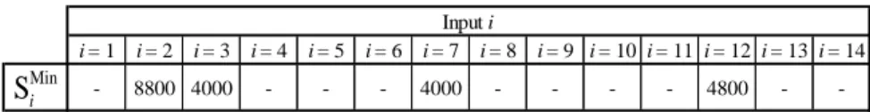
This static analysis shows that input 7 is required to produce outputs 1 (10% minimum) and 2 (10% minimum). Therefore, in order to manufacture 40,000 tons (weekly average production) to cater to an urgent unforeseen order for any product, we need to have 4,000 tons (10% of 40,000) of input 7 in stocks. The ceiling level for minimal required amounts of each input can be analyzed as a security stock in uncertain environment. The lack of such a security stock for input 7 prevents any production of both outputs 1 and 2. Table 3 shows the corresponding level of security stock for each input. We can add that any input may be used to produce any output, as the maximum yielded by optimization is higher than 0.

Blending flexibility implies absence of a BOM linking merchantable ores to extracted ores, knowing that any extracted ore may be used to produce any merchantable ore. Thus it is more efficient and effective to manage risk at extracted ore level.

Table 3: Minimal stock Min

Si of input i

This risk strategy, designed to address an urgent and unexpected order, relies on: i) security stocks for indispensable inputs to manufacture certain outputs and ii) the flexibility provided by dynamic blending to adjust output composition according to demand characteristics, combined with immediately available input stocks and availability of feeding stocks from source ores ready to be removed from the mine over the next few weeks (formulation in §2.2.a). For all these reasons, we coined the term “flexi-security

stocks” that reflects both types of risk coverage in uncertain environment. Nevertheless, note that there

remains a risk that one will not be able to fulfill an order as other (optional) inputs may not be available in sufficient quantity to produce one of the possible alternative blends.

2.2. Dynamic blending with security stocks

The risk of being unable to fulfill an unforeseen order of any merchantable ore in an amount corresponding to one week’s output, is partly addressed by dynamic blending (§2.2.1) and by security stocks, as defined above. In §2.2.2, we describe a protocol for an illustration of the proposed approach. Please note that we do not need to prove the superiority of managing risk with security stocks under managing without them. Where available quantity of an input is under the security stock, it will not be possible to satisfy the corresponding urgent and unexpected order for some outputs based on information given in Table 2. If these quantities are available, it may be possible that the substitutability offered by the blending in using available extracted ores is not adequate to meet all urgent and unexpected orders for all of the outputs.

2.2.1. Dynamic blending modelling

To evaluate the benefits of security stocks, we examine the blending problem in its dynamic form based on splitting time into periods

(

t 

1,...,T)

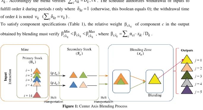
and taking into account feeding of inputs as a decision to make [1]. The problem concerns the fulfilment of a set of K production orders

(

k 

1,...,K)

already scheduled on parallel blending processors. Each order will be satisfied by a blend of inputs available in a secondary stock of source ores in the blending zone. This stock is supplied from a primary stock of source ores in the mine (Figure 1). Each order k consists of an amount

D

_k of output

j





_k

(1





_k



J)

. We note

x

_ik

i = 1 i = 2 i = 3 i = 4 i = 5 i = 6 i = 7 i = 8 i = 9 i = 10 i = 11 i = 12 i = 13 i = 14

- 8800 4000 - - - 4000 - - - - 4800 -

-Input i Min

k



. Accordingly the blend verifies _ik

D

_k

,

i

x 



k



. The schedule authorizes withdrawal of inputs to fulfill order k during periods t only where

δ

_kt



1

(otherwise, this boolean equals 0); the withdrawal time of order k is noted ν_k

(

δ

_kt

ν )

_k

t





.

To satisfy component specifications (Table 1), the relative weight β _λ

k

c of component c in the output obtained by blending must verify

β

_λ

β

_λ

β

_λ

k

k k

Min Max

c

c

<

<

c , where

β

ck





c

α

ci



x

ik

/ D

k.

Figure 1: Center Axis Blending Process

Stock

S

_it of input i, defined at the end of period t is initialized on t=0 (initial stocks

S

_i0). Its supply is linked with the binary variable

z

_it, which equals 1 only if

S

_it is fed during period t. Stock feeding is constrained by the number of conveyors

R

_tavailable at each period t, enforced by relation (1), which operate at a constant flow rate ρ . Assuming that a conveyor can only supply one input during a single period t, the amount that can be conveyed and stored in

S

_it is ρz_it. Furthermore, supplies have to comply with available source ores on the mine. In the programming horizon retained (four to six weeks), there is no constraint on removing ores lying on site in order to access lower layers [2]. The possible existence of such constraints leads to additional relations (not included in this paper) to force a minimal use of certain source ores at a particular term. That said, considering such availabilities and their daily change, we define at the beginning of the period t, availability accumulation

B

_it of source ore i stacked on the mine (without considering withdrawals), which leads to relation (2). It is assumed here that all ores transported on trucks from stocks of source ores ready to be stacked during a period feed stocks

S

_it

during this period (no intermediate stock). Therefore, flow conservation constraints are represented in relations (3) and (4). it

R ;

t

1,...,T

i

z



t





(1) 1 ρ. t_t tzit B ;it t 1,...,T; i 1,...,I      



(2) 1 ρ ₁δ .( / τ ); 1,...,I; 1,...,T  _    



K   it it it _k kt ik k S S z x i t (3) 0; 1,...,I; 1,...,T    it S i t (4)

Stocks feeding is also bound with a maximal storage capacity SMaxregarding all input stocks (5) and a security stock SMin_i for each input i (6), as defined in §2.1.

Max S ; 1,...,T it iS  t



(5) Min S ; 1,...,I; 1,...,T it i S  i t (6)

(6) can be replaced with (7) which penalizes the non-fulfilment of security stock levels for some inputs with a relative cost

w

_i (not taken into consideration in the objective-function and in the numeric illustration).

Min

0,

,

,

,

it it i it

w

i t

w

S

S

i t

 







(7)

The model used here enables outputs composition to be as close as possible to specifications at upper and lower boundaries (according to technical considerations). The general objective of this model is to stabilize the composition of merchantable ores used to manufacture phosphoric acid in order to avoid additional costs created by frequent setups of these lines (which is related to variability of upstream output composition). Relations (8) and (9) enable to determine the gap between order composition and the upper or lower structure boundaries regarding component c of output

λ

_k (only component c=1 has to be evaluated for its minimal threshold).

inf inf inf

λ λ

α

β

D ,

| β

0

k k

ck i ci

x

ik c k

k

c

 













; c 1; k1,..., K (8)

sup sup sup

λ λ

β

D

α

,

| β

0

k k

ck c k i ci

x

ik

k

c

 













; c 2,..., C; k1,..., K (9)

The optimization criterion chosen here is the minimization of the sum of those deviances related to orders that concern outputs for internal use (10). We consider that each component’s deviance has the same marginal cost θ . The objective function is derived as follows:



_θ.( sup inf₎



ck ck

k c

Min

 

   (10)

with 𝑐 = 1, … ,5 and 𝑘 ∈ 𝐾0, 𝐾0 the subset of orders produced for acid lines.

2.2.2. Test protocol analysis

We now turn to the possibility of adjusting the production schedule by changing the order of the following week just before its beginning. We compare two cases of dynamic blending practice, one without security stocks and the other with security stocks, using real programming values over one month. This comparison serves to illustrate our proposed approach. It does not amount to a demonstration by simulation to prove the superiority of the use of security stocks, which is obvious, since without them, certain unexpected orders may be impossible to produce. Our example shows the impact of unexpected orders to be fulfilled in the two cases being compared. Note again, that safety security stocks do not guarantee that all unexpected orders can be satisfied.

The problem at hand addresses the need to meet some production orders to be scheduled over a few weeks in a rolling programming approach. The schedule can be revised weekly given a one-month visibility. Two scenarios are proposed: case I is the benchmark case, where initial stocks of inputs

S

_i0 are the actual stocks and the constraints of security stocks (6) are not taken into account. In case II, we assume that initial stocks are at least equal to the security stocks level (which corresponds to

Min 0

Max(S_i ;S_i )), and that optimization is performed with a view to maintaining these levels (hence (6) is taken into account). In other words, case I reflects current OCP management, using dynamic blending, and case II assesses the value of security stocks. The idea is to show the relative performance of each case in a risk situation.

In both cases, the optimal solution is given in terms of inputs consumption and stocks feeding based on a daily time bucket. Leaving production risks aside, we assume that at some point in the planning (after one or two weeks to avoid excessive dependency of the scenario on the initial state), we receive an unexpected order to be satisfied immediately. For example, if the emergency order arrives at the end of week 2, then the order portfolio is updated and the new order is scheduled in week 3 while the order scheduled for that week is cancelled or postponed along with the following ones. To this end, we have to retain inputs stock situation

S

_it at the end of week 2 as well as the availability accumulation

B

_it on site at the beginning of week 3 in order to address another problem starting from week 3. Two variants of unexpected situations, the most likely ones, have been reviewed in this study:

- Variant A: replacing an order for an output intended for a spot market by another meant for internal use; - Variant B: postponing orders by a few days to include an order for an output intended for the spot

market.

In all variants, we do not consider any new information beyond the horizon adopted, even if shifting orders implies exceeding it. In fact, we do not extend availability accumulation

B

_iton the site as our extraction process is a LIFO system [2]. In section §3 we compare the two scenarios (with and without

3. Numerical analysis

In this section, we illustrate the flexibility offered by the availability of security stocks for the blending of 4 orders manufactured on a single blending unit over 28 days (planning horizon T). The input stocks are supplied by two conveyors with a flow rate (ρ ) of 4,000 units per day. The deviance is in tons and the marginal cost in the objective function is θ =100.

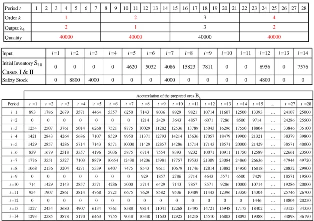
Reference problem data (before urgent unexpected order) is given in Table 4 and optimal solutions are shown in Table 5, the source ore feeding being different in the two cases at hand.

Table 4 : Reference problem data

Table 5 : Optimal solution of the reference problem

Period t 1 2 3 4 5 6 7 8 9 10 11 12 13 14 15 16 17 18 19 20 21 22 23 24 25 26 27 28 Order k Output k Qunatity 40000 40000 40000 40000 2 1 2 3 4 1 3 2 Input i =1 i =2 i =3 i =4 i =5 i =6 i =7 i =8 i =9 i =10 i =11 i =12 i =13 i =14 Initial Inventory Si 0 Cases I & II 0 0 0 0 4620 5032 4086 15823 7811 0 0 6956 0 7576 Safety Stock 0 8800 4000 0 0 0 4000 0 0 0 0 4800 0 0 Period t =1 t =2 t =3 t =4 t =5 t =6 t =7 t =8 t =9 t =10 t =11 t =12 t =13 t =14 t =15 … t =27 t =28 i =1 893 1786 2679 3571 4464 5357 6250 7143 8036 8929 9821 10714 11607 12500 13393 … 24107 25000 i =2 0 0 0 0 0 0 0 1214 2429 3643 4857 6071 7286 8500 9714 … 24286 25500 i =3 1254 2507 3761 5014 6268 7521 8775 10029 11282 12536 13789 15043 16296 17550 18804 … 33846 35100 i =4 1421 2843 4264 5686 7107 8529 9950 11371 12793 14214 15636 17057 18479 19900 21321 … 38379 39800 i =5 1429 2857 4286 5714 7143 8571 10000 11429 12857 14286 15714 17143 18571 20000 21429 … 38571 40000 i =6 839 1679 2518 3357 4196 5036 5875 6714 7554 8393 9232 10071 10911 11750 12589 … 22661 23500 i =7 1776 3551 5327 7103 8879 10654 12430 14206 15981 17757 19533 21309 23084 24860 26636 … 47944 49720 i =8 1068 2136 3204 4271 5339 6407 7475 8543 9611 10679 11746 12814 13882 14950 16018 … 28832 29900 i =9 0 0 0 0 0 0 0 929 1857 2786 3714 4643 5571 6500 7429 … 18571 19500 i =10 714 1429 2143 2857 3571 4286 5000 5714 6429 7143 7857 8571 9286 10000 10714 … 19286 20000 i =11 954 1907 2861 3814 4768 5721 6675 7629 8582 9536 10489 11443 12396 13350 14304 … 25746 26700 i =12 0 0 0 0 0 0 0 0 0 0 0 0 0 0 1446 … 18804 20250 i =13 1227 2454 3680 4907 6134 7361 8588 9814 11041 12268 13495 14721 15948 17175 18402 … 33123 34350 i =14 1293 2585 3878 5170 6463 7755 9048 10340 11633 12925 14218 15510 16803 18095 19388 … 34898 36190 Accumulation of the prepared ores Bit

Case I Case II Case I Case II Case I Case II Case I Case II Case I Case II Case I Case II Case I Case II Case I Case II

i =1 0 0 3189 2398 91 0 720 720 0% 0% 8% 6% 0% 0% 2% 2% i =2 0 0 0 0 0 1937 0 0 0% 0% 0% 0% 0% 5% 0% 0% i =3 0 4954 16000 11046 0 0 13782 13782 0% 12% 40% 28% 0% 0% 34% 34% i =4 0 0 0 0 0 0 0 0 0% 0% 0% 0% 0% 0% 0% 0% i =5 11622 4240 6989 19110 2009 1270 0 0 29% 11% 17% 48% 5% 3% 0% 0% i =6 7013 8806 0 0 0 226 0 0 18% 22% 0% 0% 0% 1% 0% 0% i =7 7000 12000 7826 7109 0 521 24371 24371 18% 30% 20% 18% 0% 1% 61% 61% i =8 10000 10000 0 0 0 0 0 0 25% 25% 0% 0% 0% 0% 0% 0% i =9 1366 0 0 0 6445 7811 0 0 3% 0% 0% 0% 16% 20% 0% 0% i =10 0 0 0 0 6873 0 1127 1127 0% 0% 0% 0% 17% 0% 3% 3% i =11 0 0 5995 338 2005 0 0 0 0% 0% 15% 1% 5% 0% 0% 0% i =12 3000 0 0 0 0 8000 0 0 8% 0% 0% 0% 0% 20% 0% 0% i =13 0 0 0 0 5467 2736 0 0 0% 0% 0% 0% 14% 7% 0% 0% i =14 0 0 0 0 17111 17500 0 0 0% 0% 0% 0% 43% 44% 0% 0% Sum 40000 40000 40000 40000 40000 40000 40000 40000 100% 100% 100% 100% 100% 100% 100% 100% k = 2 k = 3 k = 4 xik / Dk (%) xik (tonne) k = 1 k = 2 k = 3 k = 4 k = 1

The analysis of the optimal solution for case I reveals that for critical input 2, we started the simulation with a no initial inventory. Therefore, this input has largely fed our inputs stocks (for case I 32,000 and for case II only 8,000) and was used in excess of the necessary minimal quantities, thus building excess security stock. The comparison of total ore feeding between the two cases shows that case II required 16,000 tons more than case I. This is explained by: i) in case I, we started with an initial inventory that we didn’t try to maintain security stock, unlike in the second case; ii) the total deviance of internal output for case I is somewhat better than in case II, which is allowed by an increase of input feeding.

We consider that, in period 14, we received these urgent orders after completing the first two orders. We reviewed the possibility of satisfying orders at the beginning of period 15 (scenarios A and B). So, our initial inventory for both scenarios was equal to the inventory at the end of period 14 (S_{i t, 14} ). As explained in section §2.2.b, B_{i t,>28}B_{i t,28} for the scenario B.

Concerning the determination of the aggregated available ores

B

_it, we have to subtract from period 15 the amount of prepared ores used to feed our stock of inputs. The new B_it becomes

14 , 14 ₁

B_it B_{i t} ρ



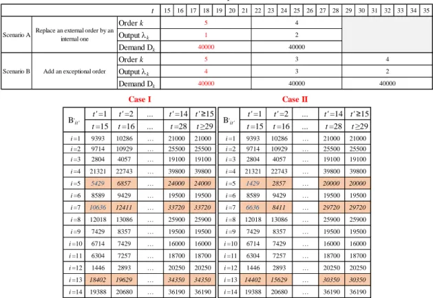
__ z_i , with T28 14 14  (scenario A) or T35 14 21(scenario B). Table 6 shows the new composition of prepared ores B_it _'for both cases and a summary of the scenarios reviewed. t =1 t =2 t =3 t =4 t =5 t =6 t =7 t =8 t =9 t =10 t =11 t =12 t =13 t =14 t =15 t =16 t =17 t =18 t =19 t =20 t =21 t =22 t =23 t =24 t =25 t =26 t =27 t =28 Sum i =1 0 0 0 0 0 0 0 4000 0 0 0 0 0 0 0 0 0 0 0 0 0 0 0 0 0 0 0 0 4000 i =3 0 0 0 0 0 4000 4000 0 0 0 4000 0 4000 0 0 0 0 0 0 0 0 4000 4000 4000 0 0 0 4000 32000 i =5 0 0 4000 0 0 4000 0 0 4000 0 0 4000 0 0 0 0 0 0 0 0 0 0 0 0 0 0 0 0 16000 i =6 0 0 0 0 4000 0 0 0 0 0 0 0 0 0 0 0 0 0 0 0 0 0 0 0 0 0 0 0 4000 i =7 0 0 4000 0 4000 0 0 0 4000 0 4000 0 0 0 0 0 0 0 0 0 4000 4000 4000 4000 4000 4000 4000 0 44000 i =8 0 0 0 4000 0 0 0 0 0 0 0 0 0 0 0 0 0 0 0 0 0 0 0 0 0 0 0 0 4000 i =10 0 0 0 0 0 0 0 0 0 0 0 0 0 4000 0 0 0 4000 0 0 0 0 0 0 0 0 0 0 8000 i =11 0 0 0 0 0 0 0 4000 0 0 0 4000 0 0 0 0 0 0 0 0 0 0 0 0 0 0 0 0 8000 i =13 0 0 0 0 0 0 0 0 0 0 0 0 0 0 4000 0 0 0 0 4000 0 0 0 0 0 0 0 0 8000 i =14 0 0 0 0 0 0 0 0 0 0 0 0 0 0 0 4000 4000 4000 4000 4000 0 0 0 0 0 0 0 0 20000 148000 t =1 t =2 t =3 t =4 t =5 t =6 t =7 t =8 t =9 t =10 t =11 t =12 t =13 t =14 t =15 t =16 t =17 t =18 t =19 t =20 t =21 t =22 t =23 t =24 t =25 t =26 t =27 t =28 Sum i =1 0 0 0 0 0 0 0 4000 0 0 0 0 0 0 0 0 0 0 0 0 0 0 0 0 0 0 0 0 4000 i =2 0 0 0 0 0 0 0 0 0 0 0 0 0 0 0 0 0 0 0 4000 4000 0 0 0 0 0 0 0 8000 i =3 0 0 0 0 0 4000 4000 0 0 0 0 4000 4000 0 0 0 0 0 0 0 0 0 0 4000 4000 4000 4000 0 32000 i =5 0 0 0 0 0 0 0 4000 4000 4000 0 4000 0 4000 0 0 0 0 0 0 0 0 0 0 0 0 0 0 20000 i =6 0 0 0 0 4000 0 0 0 0 0 0 0 0 0 0 0 0 0 0 0 0 0 0 0 0 0 0 0 4000 i =7 0 0 4000 0 4000 0 4000 0 0 0 4000 0 0 4000 0 0 0 0 0 0 0 4000 4000 4000 4000 0 4000 4000 44000 i =8 0 0 0 4000 0 0 0 0 0 0 0 0 0 0 0 0 0 0 0 0 0 0 0 0 0 0 0 0 4000 i =10 0 0 0 0 0 0 0 0 0 0 0 0 4000 0 0 0 0 0 0 0 0 0 4000 0 0 0 0 0 8000 i =11 0 0 0 0 0 4000 0 0 4000 0 0 0 0 0 0 0 0 0 0 0 0 0 0 0 0 0 0 0 8000 i =12 0 0 0 0 0 0 0 0 0 0 0 0 0 0 0 0 0 0 4000 0 4000 0 0 0 0 0 0 0 8000 i =13 0 0 0 0 0 0 0 0 0 0 4000 0 0 0 0 4000 0 0 0 0 0 0 0 0 0 0 0 0 8000 i =14 0 0 0 0 0 0 0 0 0 0 0 0 0 0 0 0 4000 4000 4000 4000 0 0 0 0 0 0 0 0 16000 164000 Case I ρ*zit Period Input Case II ρ*zit Period Input c =1 c =2 c =3 c =4 c =5 Internal Output Deviance Internal Output Deviance Internal Output Deviance Internal Output Deviance Internal Output Deviance k = 1 967.51 560.00 71.13 1419.32 492.43 3510.38 k = 2 0.00 560.00 93.96 115.74 0.00 769.70 k = 4 0.00 91.22 0.00 391.38 0.00 482.60 k = 1 586.21 454.26 36.34 829.36 303.88 2210.05 k = 2 0.00 560.00 78.48 715.59 0.00 1354.07 k = 4 _{0.00 91.22 0.00 391.38 0.00 482.60} II Yes Case Constraint on Security Stock Internal orders Internal Output Total Deviance I No

Table 6 : Scenario problems data

The differences observed for B_it _' between cases I and II are due to the difference in total ore feedings for the first 14 periods. The optimal solutions for each scenario considering the two cases are presented in Table 7.

Table 7 : Optimal solutions x_ij

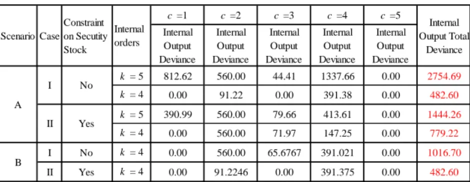
The results obtained by the optimization model concerning our criteria (10) for the different scenarios and cases are grouped in Table 8. In case I, the total deviance of order 2 concerning internal output 1 in the reference solution is of approximately 770T (Table 5) while the deviance of order 5 concerning the same internal output in scenario A is approximately 2,755T (Table 8). This difference is explained by the stock level of indispensable inputs at the end of period 14 and the cumulated availability B_it _' for these critical

15 16 17 18 19 20 21 22 23 24 25 26 27 28 29 30 31 32 33 34 35 Order k Output k Demand Dk Order k Output k Demand Dk 1 t Scenario A Replace an external order by an

internal one

Scenario B Add an exceptional order 4 40000 3 4 5 40000 2 5 40000 40000 3 2 4 40000 t' =1 t' =2 … t' =14 t' ≥15 t' =1 t' =2 … t' =14 t' ≥15 t =15 t =16 … t =28 t ≥29 t =15 t =16 … t =28 t ≥29 i =1 9393 10286 … 21000 21000 i =1 9393 10286 … 21000 21000 i =2 9714 10929 … 25500 25500 i =2 9714 10929 … 25500 25500 i =3 2804 4057 … 19100 19100 i =3 2804 4057 … 19100 19100 i =4 21321 22743 … 39800 39800 i =4 21321 22743 … 39800 39800 i =5 5429 6857 … 24000 24000 i =5 1429 2857 … 20000 20000 i =6 8589 9429 … 19500 19500 i =6 8589 9429 … 19500 19500 i =7 10636 12411 … 33720 33720 i =7 6636 8411 … 29720 29720 i =8 12018 13086 … 25900 25900 i =8 12018 13086 … 25900 25900 i =9 7429 8357 … 19500 19500 i =9 7429 8357 … 19500 19500 i =10 6714 7429 … 16000 16000 i =10 6714 7429 … 16000 16000 i =11 6304 7257 … 18700 18700 i =11 6304 7257 … 18700 18700 i =12 1446 2893 … 20250 20250 i =12 1446 2893 … 20250 20250 i =13 18402 19629 … 34350 34350 i =13 14402 15629 … 30350 30350 i =14 19388 20680 … 36190 36190 i =14 19388 20680 … 36190 36190 B'it' Case I Case II B'it' Case I II I II I II I II I II Order k Output k i =1 3397 3816 720 7725 9036 882 371 0 7404 720 i =2 0 0 0 0 11200 15008 2548 1792 0 0 i =3 0 10667 13782 9333 0 2031 0 0 7320 13782 i =4 0 0 0 0 0 0 0 0 0 0 i =5 14009 4445 0 824 259 0 0 0 5750 0 i =6 1215 0 0 0 1740 0 0 0 0 0 i =7 9707 9128 24371 11417 49 0 0 520 11125 24371 i =8 0 0 0 0 0 0 0 0 0 0 i =9 0 0 0 0 6445 0 0 2322 0 0 i =10 0 0 1127 0 0 0 4000 2873 0 1127 i =11 11673 11944 0 10701 1363 18272 0 0 8402 0 i =12 0 0 0 0 0 3807 0 993 0 0 i =13 0 0 0 0 0 0 12928 14000 0 0 i =14 0 0 0 0 9907 0 20153 17500 0 0 Demand Dk 40000 40000 40000 40000 40000 40000 40000 40000 40000 40000 Scenario A 5 4 1 2 Scenario B 3 5 4 3 2 4

inputs. On the other hand, the deviance of the same order in case II is approximately 779T due to the presence of security stock for the indispensable inputs. The analysis of the total deviance shows that the max optimal deviance for internal output (j=1) is 432T. The max deviance obtained by introducing both scenarios in the absence of security stock (case I) for the same output is approximately 2,755 T, while this value becomes 1,444 T for case II where we consider the constraint on safety stocks. For the other internal output (j=2), the max optimal deviance is 567 T. In case I the max deviance achieved is 1,017 T, unlike case II where this value was below 799 T.

We note that the absence of security stock (case I) greatly increases the max optimal value previously observed, whereas with case II the where security stocks enables to approximate the optimal deviances. This example demonstrates that reliance on security stocks combined with the use of the dynamic blending approach enables coping with unexpected situations with maximum flexibility. Remember that this example is provided for illustration purposes and does not amount to a demonstration of the superiority of a solution with security stock, which, as noted above, is logically obvious ().

Table 8 : Total internal deviance

4. Conclusion

In this article we propose a new dynamic blending method linked to minimum stock build up, tested in the case of a mining chain, to control risk related to demand volatility. These security stocks are defined only for critical source ores to enable a week’s production of any output. This work has led to sizing minimal stocks to be built up in an uncertain universe and has enabled us to define an optimization criterion relevant to the mining sector. Finally, for different scenarios, it has enabled to define the minimum stock levels in relation to the objective variable.

To conclude, our study points to research avenues regarding: i) refining the objective function by taking into account a marginal cost of deviance per component (as defined by constraint (7)), and ii) introducing constraints on some input removals from the mine in order to free up access to lower mine layers that are planned to be extracted.

5. References

1. Azzamouri, A., Giard, V.: Dynamic blending as a source of flexibility and efficiency in controlling phosphate supply chain. Cahier de recherche 381 du LAMSADE (2017).

2. Azzamouri, A., Fenies, P., Fontane, F., Giard, V.: Scheduling of Open-pit Phosphate Mine Extraction, accepted for publication in International Journal of Production Research (2018).

3. Graves, S.C. and Willems, S.P.: Supply Chain Design: Safety Stock Placement and Supply Chain Configuration, Handbooks in Operations Research and Management Science, Elsevier, Volume 11, 95-132 (2003).

4. Inderfurth, K. and Vogelgesang, S.: Concepts for safety stock determination under stochastic demand and different types of random production yield, European Journal of Operational Research, Volume 224, Issue 2, 293-301 (2013).

5. Keen, P.G.W. and Scott Morton, M.S.: Decision support system: an organizational perspective. Addison.Wesley (1978).

6. Van Kampen, T. J., van Donk, D. P., & van der Zee, D.-J.: Safety stock or safety leadtime: Coping with unreliability in demand and supply. International Journal of Production Research, 48, 7463–7481 (2010).

c =1 c =2 c =3 c =4 c =5 Internal Output Deviance Internal Output Deviance Internal Output Deviance Internal Output Deviance Internal Output Deviance k = 5 812.62 560.00 44.41 1337.66 0.00 2754.69 k = 4 0.00 91.22 0.00 391.38 0.00 482.60 k = 5 390.99 560.00 79.66 413.61 0.00 1444.26 k = 4 0.00 560.00 71.97 147.25 0.00 779.22 I No k = 4 0.00 560.00 65.6767 391.021 0.00 1016.70 II Yes k = 4 0.00 91.2246 0.00 391.375 0.00 482.60 B Scenario Case Constraint on Secutity Stock Internal orders Internal Output Total Deviance A I No II Yes