HAL Id: hal-00429900
https://hal.archives-ouvertes.fr/hal-00429900
Submitted on 5 Nov 2009
HAL is a multi-disciplinary open access
archive for the deposit and dissemination of
sci-entific research documents, whether they are
pub-lished or not. The documents may come from
teaching and research institutions in France or
abroad, or from public or private research centers.
L’archive ouverte pluridisciplinaire HAL, est
destinée au dépôt et à la diffusion de documents
scientifiques de niveau recherche, publiés ou non,
émanant des établissements d’enseignement et de
recherche français ou étrangers, des laboratoires
publics ou privés.
Smart Ion-Selective Electrode Arrays
Leonardo Tomazeli Duarte, Christian Jutten, Saïd Moussaoui
To cite this version:
Leonardo Tomazeli Duarte, Christian Jutten, Saïd Moussaoui. A Bayesian Nonlinear Source
Separa-tion Method for Smart Ion-Selective Electrode Arrays. IEEE Sensors Journal, Institute of Electrical
and Electronics Engineers, 2009, 9 (12), pp.1763-1771. �10.1109/JSEN.2009.2030707�. �hal-00429900�
A Bayesian Nonlinear Source Separation Method
for Smart Ion-selective Electrode Arrays
Leonardo T. Duarte, Student Member, IEEE, Christian Jutten, Fellow, IEEE, and Sa¨ıd Moussaoui
Abstract—Potentiometry with ion-selective electrodes (ISEs)
provides a simple and cheap approach for estimating ionic activities. However, a well-known shortcoming of ISEs regards their lack of selectivity. Recent works have suggested that smart sensor arrays equipped with a blind source separation (BSS) algorithm offer a promising solution to the interference problem. In fact, the use of blind methods eases the time-demanding calibration stages needed in the typical approaches. In this work, we develop a Bayesian source separation method for processing the outputs of an ISE array. The major benefit brought by the Bayesian framework is the possibility of taking into account some prior information, which can result in more realistic solutions. Concerning the inference stage, it is conducted by means of Markov chain Monte Carlo (MCMC) methods. The validity of our approach is supported by experiments with artificial data and also in a scenario with real data.
Index Terms—Blind source separation, ion-selective electrode,
chemical sensor array, Bayesian approach.
I. INTRODUCTION
I
ON-selective electrodes (ISEs) [2], [3], [4] are devices used for estimating the ionic activity, a measure of effective concentration of an ion in aqueous solution. The transducer mechanism in an ISE is based on a sensitive membrane in which the electrochemical potential depends on the concen-tration of a given charged chemical specie. A typical example of ISE is the glass electrode used for measuring the pH value. Moreover, ISEs for ions such as ammonium, potassium, and calcium are of great interest in applications like water quality control [5] and biomedical monitoring [6], [7].The most relevant drawback of an ISE concerns its lack of selectivity, that is, an ISE may respond to interfering ions other than the target one. While in some situations the interference process can be negligible, there are other cases in which this problem seems to be more accentuated, especially if the ions under analysis have similar physicochemical properties. If no care is taken in these cases, the measurements provided by the ISE may become uncertain.
A possible way to overcome the interference problem relies on the concept of smart sensor array (SSA). In a SSA, the data acquisition is done through several ISEs. Then, the desired information is extracted by a data processing block that tries to exploit the diversity provided by the array. Typically, the
Leonardo T. Duarte and C. Jutten are with the GIPSA-lab (UMR CNRS 5216), Institut Polytechnique de Grenoble, Grenoble, France (e-mail: [email protected], [email protected]). C. Jut-ten is also with Institut Universitaire de France.
Sa¨ıd Moussaoui is with IRCCyN (UMR CNRS 6597), Ecole Centrale Nantes, Nantes, France (e-mail:[email protected]).
A preliminary version of this paper [1] was presented at the 8th International Conference on Independent Component Analysis and Signal Separation (ICA 2009) and was published in its proceedings.
development of a SSA follows a supervised paradigm, i.e. a set of training (or calibration) samples is used to adjust the parameters of the SSA data processing block. Despite the good results obtained in both quantitative and qualitative analysis (for example, see the electronic tongues [8]), supervised meth-ods suffers from two practical problems: 1) the acquisition of a sufficient number of training samples may be time-demanding, and 2) the calibration procedure must be performed from time to time due to the sensor’s drift. These limitations are the main motivations for the use of unsupervised (or blind) methods. In this new case, the SSA data processing block only uses the array responses and some parametric knowledge on the interference process. Therefore, the calibration stage may be skipped or, at least, quite reduced.
In this work, we are interested in the problem of unsu-pervised quantitative analysis via an ISE array, which can be expressed as follows: there is a set of source signals, each one representing the activity of a given ion. Due to the interference phenomena in the transduction stage, the signals recorded by the ISE array are mixed versions of the sources. Then, our goal is to retrieve the sources using only the ISE array outputs. This description is an example of a Blind Source Separation problem (BSS) [9], [10], to which the signal processing community has been devoting a great deal of attention. The main difficulty in the application of BSS methods to the problem treated in this work stems from the nonlinear behavior of an ISE. While linear BSS is now a well established matter, the more general problem of nonlinear BSS is still a very challenging one (see [11]).
The first studies [12], [13], [14] on the design of BSS methods for chemical sensor arrays were based on Independent Component Analysis (ICA) methods [9]. Despite the encour-aging results presented in these works, the developed methods have several limitations. Firstly, they do not take into account some prior information that would be useful for improving the separation quality. For instance, the sources in our problem are always non-negative, since they represent ionic activities. Secondly, given that ICA methods works with the assumption that the sources are statistically independent, they cannot be used when the sources are correlated. Finally, all these works were evaluated with synthetic data in noiseless situations.
In this paper, we propose a Bayesian source separation method for processing the outputs of an ISE array. The Bayesian approach has been proved to be attractive in several domains including audio source separation [15] and spec-troscopy data analysis [16]. Moreover, one of the main advan-tages of this approach is exactly the possibility of incorporat-ing prior information into our method and of workincorporat-ing in noisy scenarios. Finally, the advent of sampling techniques [17] such
as Monte Carlo Markov Chain (MCMC) methods has provided an efficient solution to the calculation of the complex integrals that are usually associated with a Bayesian framework.
This work is an extended version of the conference pa-per [1], which only contained the basics of our method and some preliminary results. In the present version, we detail important aspects of our method and widely expand the results section, including a comparison with a supervised technique. Concerning the paper’s organization, we start with a descrip-tion of the mixing model associated with the applicadescrip-tion in mind. After that, in Section III, we describe the building blocks of our Bayesian source separation scheme. In Section IV, we conduct some experiments with artificial and real data to assess the performance of our proposal. Finally, our conclusions are presented in Section V.
II. PROBLEMSTATEMENT
Let us consider a solution containing ns ions and an array
composed of nc electrodes. Due to the interference problem,
the response of the i-th ISE within the array at the instant t, represented by yit, is dependent not only on the activity of its
target ion, sit, but also on the activities of the other ions in
the solution, sjt. According to the Nicolsky-Eisenman (NE)
equation [3], this phenomenon can be modeled as1 yit= ei+ dilog sit+ ns X j=1,j6=i aijszjti/zj , (1)
where ei is a constant, zj is the valence of the j-th ion and
aij denotes the selectivity coefficients. Finally, di = RT /ziF ,
where R is the gas constant, T the temperature in Kelvin, and F the Faraday constant. When the valences of the ions under analysis are the same, the model (1) becomes a particular case of the class of post-nonlinear (PNL) models [13]. Nonetheless, when the valences are different and the ISEs within the array have different ions as targets, the resulting model becomes tougher due to the appearance of a nonlinearity inside the logarithm term [14].
By arranging the response of each ISE within the array, the mixing process can be expressed as follows:
Y = e · 11×nd+ diag(d) log (A ⊗
zS) , (2)
where nd corresponds to the number of available samples,
Y ∈ Rnc×nd, e = [e1, . . . , e nc] T, d = [d1, . . . , d nc] T, A ∈ Rnc×ns
+ and S ∈ Rn+s×nd. The element it of Y corresponds to yitand therefore the i-th row of Y corresponds to the time
response of the i-th ISE within the array. Analogously, the element jt of S denotes the activity of the j-th ion at the instant t, i.e. sjt. Matrix A contains the selectivity coefficients.
The vector of valences is denoted by z = [z1, . . . , zns]
T,
and the operator ⊗z describes the nonlinear transformation inside the logarithm function present in the NE model (see Eq. (1)). If the valences zi are equal, then ⊗z results in a
simple matrix multiplication. Finally, 11×nd corresponds to a
vector (dimension nd) with all elements equal to one.
1In this work, log and ln stands for the logarithm of base 10 and the natural
logarithm, respectively.
In view of a possible model inaccuracy and/or of the errors introduced by the measurement system, a more realistic description for the array outputs is given by:
X = Y + N, (3)
where N ∈ Rnc×nd represents the noise terms. We assume
a zero mean additive white Gaussian noise (AWGN) with covariance matrix Cn= diag(σ2), where the elements of the vector σ2, the variances σ2
1, . . . , σn2c, are unknown.
With equations (2) and (3) in mind, we may formulate the source separation problem treated in this work: given the array response X and assuming that the valences zi are known, our
goal is to estimate the elements of S (ionic activities). Since we envisage a blind method, the other parameters related to the mixing model (except z) and the noise variance at each electrode are also unknown and, thus, should be estimated. Furthermore, as it will become clear later, there are other unknown parameters, denoted by φ, which are related to the prior distributions assigned to the sources. Henceforth, all these unknown parameters will be represented by the vector θ = [S, A, d, e, σ, φ] and the following notation will be adopted: θ−θq represents the vector containing all elements
of θ except θq.
III. BAYESIANSOURCESEPARATIONMETHOD The first step in Bayesian estimation is to assign an a priori probability distribution function, or simply prior, for each unknown parameter. This is done based on some available knowledge or constraint related to the unknown parameters; in Section III-A, we will discuss how this step can be accomplished in our problem. Later, in Section III-B, we will present the likelihood function p(X|θ) resulting from the mixing model (Eqs. (2) and (3)). Then, in Section III-C, we shall derive the posterior distribution, which can be seen as an update of the priors using the information brought by the likelihood function. According to the Bayes’ rule, the posterior is given by p(θ|X) = p(X|θ)p(θ)/p(X). Given that p(X) is not a function of the unknown parameters θ, we are mainly interested in the following expression
p(θ|X) ∝ p(X|θ) p(θ). (4)
Finally, in Section III-D, we shall discuss how an inference scheme based on (4) can be set to resolve our nonlinear source separation problem.
A. Defining the prior distributions
1) Prior distribution of the sources S: We adopted log-normal distributions to model the sources. This distribution is always non-negative which seems natural in our problem as the sources represent ionic activities. Moreover, there are two other aspects that motivate our choice. Firstly, the estimation of the parameters of a log-normal distribution is not complicated. As it will be checked later, it is possible to define conjugate priors in this case2. Also, there is a practical argument behind
2From the Bayes’ rule p(X/Y ) ∝ p(Y /X)p(X). If p(X/Y ) and p(X)
belong to the same family, then p(X) is said to be conjugate with respect to the likelihood p(Y /X). When the prior is conjugate, the Bayesian inference only needs the update of the posterior distribution (see [18], for instance).
this choice. Ionic activities are expected to have a small vari-ation in the logarithmic scale. This can be taken into account by the log-normal distribution, since such a distribution is nothing but a Gaussian distribution in the logarithmic scale. In mathematical terms, the prior assigned to sjt is given by
p(sjt) ∝ 1 sjtexp à −(ln(sjt) − µj) 2 2σ2 j ! 1[0,+∞[(sjt), (5)
where µj, σj are the distribution parameters and1[0,+∞[(sjt)
is the indicator function. We assume that the samples are independent and identically-distributed (i.i.d) and also that the sources are mutually statistically independent3, that is
p(S) = ns Y j=1 nd Y t=1 p(sjt).
2) Prior distribution of the sources hyperparameters φ: The parameters φj= [µj σj] in Eq. (5) are also unknown in
our problem and, thus, priors must be defined for them. We adopted a Gaussian prior distribution for µj, that is:
p(µj) =q 1 2πσ2 µj exp à − ¡ µj− µµj ¢2 2σ2 µj ! , (6)
where µµj and σµj correspond to the hyperparameters. For
rj = 1/σ2j, a Gamma distribution is considered:
p(rj) = rαrj−1 j Γ(αrj)β αrj rj exp à −rj βrj ! 1[0,+∞[(rj), (7)
where αrj and βrj are the hyperparameters. In Section III-D, we will show that these two priors lead to conjugate pairs in the estimation of µj and rj = 1/σ2j.
3) Prior distribution of the selectivity coefficients A: According to the literature in potentiometric sensors (see [3], [19]), the selectivity coefficients are also non-negative. More-over, it is rare to find a sensor whose response depends more on the interfering ion than on the target one, that is, aijusually
lies in the interval [0, Amax] where Amax ∈ [0, 1]. Thus, an
uniform distribution can be assumed for each4 a
ij, that is
p(aij) ∝1[0,Amax](aij). (8)
If no additional information is available, one can set Amax=
1. However, it is possible to refine this information by using databases such as [19] or by incorporating some information acquired during the fabrication process. Finally, the coeffi-cients of A are assumed mutually independent, i.e.
p(A) = nc Y i=1 ns Y j=1 p(aij).
3If some information concerning a possible dependency between the sources
is available, it can be used for defining the priors. In this case, however, one goes toward a less general approach that is useful only to the modeled situation. Besides, the inference problem becomes more difficult in this case.
4In view of Eq. (1), we consider a
ij= 1 when i = j.
4) Prior distribution of the Nernstian slopes d: As already discussed, diis related to physical parameters. For a room
tem-perature, it takes approximately 0.059/zi, and the electrodes
with such sensibility are said to have a Nernstian response. However, due to the sensor fabrication process and aging, a deviation from this theoretical value is usually observed. Furthermore, even the injection scheme can play a role on the value of this parameter [20]. This possible deviation from the Nernstian value can be taken into account by setting a Gaussian prior of mean µdi= 0.059/ziV, i.e.:
p(di) ∝ exp à −(di− µdi) 2 2σ2 di ! . (9) σ2
di must be high enough to correctly model the derivations
from the theoretical value. For example, for an electrode whose target ion is monovalent, one obtains a coherent distribution by setting σdi = 0.01. Again, this knowledge could be refined
if additional information is available, or if the measurements are conducted in different temperatures. Finally, we assume that the elements of d are statistically independent.
5) Prior distribution of e: In contrast to the parameters di,
there is no theoretical value for ei. Still, as can be observed
in [2], [21], eiusually lies in the interval [0.05, 0.35]V. Hence,
the following Gaussian prior may be adopted p(ei) ∝ exp µ −(ei− µei) 2 2σ2 ei ¶ , (10)
where the mean is given by µei = 0.20V and σ
2
ei must be
de-fined so (10) goes toward a flat prior in the interval [0.05, 0.35]. The elements of e are assumed mutually independent.
6) Prior distribution of the noise variance σ2
i: A very
common approach [16], [22] is to assign inverse Gamma priors for the noise variances; that is, γi= 1/σi2is modeled through
a Gamma distribution with parameters ασi and βσi
p (γi) = γ ασi−1 i Γ(ασi)β ασi σi exp µ −γi βσi ¶ 1[0,+∞[(γi) . (11)
The motivation behind this modeling comes from the fact that it results in a conjugate pair. Moreover, it is possible to set ασi and βσi to obtain a non-informative prior [22].
B. Probabilistic modeling of the mixing process
Based on the mixing model defined in Section II and on the assumption of i.i.d. Gaussian noise which is also spatially uncorrelated, the likelihood is defined as
p(X|θ) = nd Y t=1 nc Y i=1 Nxit à ei+ dilog ³Xns j=1 aijszjti/zj ´ , σ2 i ! , (12) where Nxik(µ, σ2) denotes a Gaussian random variable in xik
C. Bayesian inference
Having defined the priors p(θ) and the likelihood p(X|θ), we may now apply the Bayes’ rule to obtain the posterior distribution p(θ|X). Given that the unknown variables of our problem are mutually independent (except S and φ), the prior distribution factorizes and, as a consequence, the posterior distribution becomes
p(θ|X) ∝ p(X|θ) p(S|φ) p(φ) p(A) p(e) p(d) p(σ). (13) This a posteriori distribution can be used in the derivation of an inference scheme to estimate the parameters of interest. For instance, one may adopt the minimum mean square error (MMSE) estimator [23], which is given by
θM M SE =
Z
θ p(θ|X)dθ. (14)
The exact implementation of this estimator is difficult because the analytical evaluation of this integral is hard in the problem considered here. Nonetheless, a good approximation of (14) can be provided by sampling methods. The idea here is to approximate the MMSE estimator using samples obtained from the posterior distribution p(θ|X). If, for instance, the generated samples are represented by θ(1), θ(2), . . . , θ(M ), then expression (14) can be approximated by
e θM M SE= 1 M M X m=1 θ(m). (15)
According to the law of large numbers, eθM M SE = θM M SE
as M → +∞. This important result gives the theoretical foundation for the above-described methodology, which is referred as Monte Carlo integration [17].
D. Gibbs sampling scheme
The implementation of the MMSE estimator boils down to the task of generating samples from p(θ|X). In this work, this is done by the Gibbs’ sampler, a Markov Chain Monte Carlo (MCMC) method tailored for simulating joint distributions. The idea in MCMC methods is to generate a Markov chain that admits the desired distribution (p(θ|X) in our case) as stationary distribution. Assuming that x ∼ p(x) stands for the sampling operation, i.e. x is a sample from the distribution p(x), then the Gibbs’ sampler can be summarized as follows:
1) Set initial samples θ(0)1 , θ(0)2 , . . . , θN(0); 2) For m = 1 to M , do θ1(m) ∼ p(θ1|θ2(m−1), θ3(m−1), , . . . , θ(m−1)N , X) θ2(m) ∼ p(θ2|θ1(m), θ(m−1)3 , . . . , θ(m−1)N , X) .. . θN(m) ∼ p(θN|θ(m)1 , θ (m) 2 , . . . , θ (m) N −1, X) end.
Note that the Gibbs’ sampler simulates a high-dimensional joint distribution by sequentially sampling from the condi-tional distribution of each variable5. Therefore, aiming at the
5Actually, the Gibbs’ sampler requires only the conditional distributions up
to a proportional gain.
implementation of the Gibbs sampler for our problem, we should obtain the conditional density for each element of θ. In the sequel, this will be accomplished by observing that
p(θq|θ−θq, X) ∝ p(X|θ)p(θq) (16)
and by considering the likelihood function (12) and the prior distributions (defined in Section III-A).
1) Conditional distributions for the sources: Substituting expressions (12) and (5) into (16), one has
p(sjt|θ−sjt, X) ∝ exp " n c X i=1 − 1 2σ2 i à xit− ei − dilog ³ aijszjti/zj + ns X b=1,b6=j aibszbti/zb ´!2 −(ln(sjt) − µj) 2 2σ2 j # 1 sjt1[0,+∞[(sjt). (17)
2) Conditional distributions for the sources hyperparame-ters φ: Because p(X|θ) is not a function of the paramehyperparame-ters φj= [µj σj], the conditional density of µj is given by
p¡µj|σj, S(j,:) ¢
∝ p¡S(j,:)|µj, σj
¢
p(µj), (18)
where S(j,:) denotes all the elements of the j-th row. By substituting (5) and (6) into (18), we obtain:
p¡µj|σj, S(j,:) ¢ ∝ nd Y t=1 " exp à −(ln(sjt) − µj) 2 2σ2 j !# exp à − ¡ µj− µµj ¢2 2σ2 µj ! . (19) The first term of (19) can be rewritten as a Gaussian function in µj, with mean µLµj = 1/nd
Pnd
t=1ln(sjt) and variance
σ2
Lµj = σ2j/nd. Thus, (19) becomes a product of two Gaussian
distributions which is also a Gaussian distribution, i.e.:
p¡µj|σj, S(j,:) ¢ ∝ exp − ³ µj− µP ostµj ´2 2σ2 P ostµj , (20) where6 σ
P ostµj = σL2µjσµ2µj/(σ2Lµj + σ2µµj) and µP ostµj =
(µLµjσ2µµj + µµµjσL2µj)/(σL2µj+ σ2µµj).
Similarly to the case of µj, the conditional density of rj =
1/σ2 j is given by p ¡ rj|µj, S(j,:) ¢ ∝ p¡S(j,:)|µj, rj ¢ p(rj).
Thus, by considering (5) and (7), one has p¡rj|µj, S(j,:) ¢ ∝ nd Y t=1 " √ rjexp ³ −0.5rj(ln(sjt) − µj)2 ´# rαjrj−1exp à −rj βrj ! 1[0,+∞[(rj). (21)
6The derivation of the mean and variance of a product of two Gaussian can
We can rewrite p(rj|µj, S(j,:)) as a Gamma distribution, i.e. p¡rj|µj, S(j,:) ¢ ∝ rjαP ostrj exp à − rj βP ostrj ! 1[0,+∞[(rj), (22)
where αP ostrj = αrj + nd/2 and β
−1
P ostrj =
³ Pnd
t=1(ln(sjt) − µj)2
´
/2βrj It is now clear that we obtain a conjugate pair and, thus, we can sample from p¡rj|µj, S(j,:)
¢
by sampling from a Gamma distribution.
3) Conditional distribution of aij: The derivation of
the conditional distribution of p(aij|θ−aij, X) is close to
the one conducted for sjt. Indeed, by considering
expres-sion (12), (16), and (8), it turns out that p(aij|θ−aij, X) ∝ exp
" − 1 2σ2 i nd X t=1 Ã xit− ei− dilog ³ aijszjti/zj + ns X b=1,b6=j aibszbti/zb ´!2# 1[0,1](aij). (23)
4) Conditional distribution of di: Using Eqs. (12) and (9),
and after some straightforward calculations, p(di|θ−di,X) can
be written as the following Gaussian distribution p(di|θ−di, X) ∝ exp − ³ di− µP ostdi ´2 2σ2 P ostdi , (24)
where σP ostdi = σ2Ldiσµ2di/(σL2di + σ2µdi), µP ostdi =
(µLdiσ2µdi+ µµdiσ2Ldi)/(σL2di+ σ2µdi), and µLdi = (Pnd t=1(xit− ei)) log ³Pns b=1aibs zi/zb bt ´ ³ log³Pns b=1aibszbti/zb ´´2 ,(25) σ2 Ldi = σ2 µdi ³ log³Pns b=1aibszbti/zb ´´2. (26)
5) Conditional distribution of ei: The development of this
expression is similar to the one performed for di. After some
calculations, it is not difficult to show that p(ei|θ−ei, X) ∝ exp
à − ¡ ei− µP ostei ¢2 2σ2 P ostei ! , (27)
where σP ostei = σ2Leiσ2µei/(σL2ei + σµ2ei), µP ostei =
(µLeiσµ2ei+ µµeiσL2ei)/(σL2ei+ σ2µei), and µLei = Pnd t=1 ³ xit− dilog ³Pns b=1aibszbti/zb ´´ nd (28) σ2 Lei = σei/nd. (29)
6) Conditional distribution of the noise variance σi: As
discussed before, the attribution of a Gamma prior for γi =
1/σ2
i culminates in a conjugate pair. Indeed, by considering
expressions (12) and (11), one can show that p(γi|θ−γi, X)
can be reduced to the following Gamma distribution: p(γi|θ−γi, X) ∝ γ αP ostσi−1 i exp à −γi βP ostσi ! 1[0,+∞[, (30)
where αP ostσi = ασi + nd/2 and β
−1 P ostσi = 1 2 Pnd t=1 ³ xit− ei− dilog ³Pns b=1aibszbti/zb ´´2 + β−1 σi . E. Algorithm Description
Let us make some remarks on the final algorithm, which is summarized in Tab. I. In a first step, we must define hy-perparameters that lead to non-informative distributions [18]. For instance, in the experiments described in Section IV, this strategy was implemented by setting the following values for the variances of the Gaussian priors: σ2
di = 0.01 and
σ2
ei = 0.03. Moreover, a high value of the parameter σ
2
µj,
which is related to the sources prior, was defined (σ2
µj = 100).
Concerning the Gibbs’ sampler, the resulting conditionals for almost all parameters are given by standard distributions (normal and Gamma) and, thus, sampling is straightforward in these cases. However, p(sjt|θ−sjt, X) and p(aij|θ−aij, X)
result in non-standard distributions, thus requiring more so-phisticated sampling methods. In this work, this task is accom-plished by the Metropolis-Hasting (MH) algorithm [17]. Based on an instrumental distribution g(x; y), the MH algorithm simulates a given distribution p(x) in an iterative fashion; given x(t), the current sample of p(x), the following iteration is done for obtaining the next sample x(t+1):
1) x∗∼ g(x; x(t)) (generation of a candidate sample); 2) Calculate a = min
³
1,p(xp(x(t)∗)g(x)g(x(t)∗;x;x(t)∗))
´ ;
3) u ← sample from a uniform distribution in [0, 1]; 4) if u ≤ a, x(t+1) = x∗ (accept the proposed sample)
else x(t+1)= x(t)(reject the proposed sample). In this work, truncated Gaussian are considered as instrumental distributions; in order to obtain good acceptance rate, we conducted, for each situation, preliminary simulations to adjust the variances of these distributions.
As the resulting Markov chain of the Gibbs’ sampler takes some time to converge to its stationary distribution, the samples obtained in a first period (burn-in period) are not taken into account by the estimator (see Eq. (31)). A simple visual inspection of the evolution of some channel states was done for determining the burn-in period. However, more sophisticated strategies for convergence monitoring can be envisaged.
A last step in our algorithm concerns a post-processing stage for dealing with the scale and translation ambiguities inherent in blind methods [10]. For example, in PNL mixtures, the best we can do is to obtain an estimation ˜sjt given by ˜sjt=
ajsjt+ bj, where aj and bj are unknown, and sjtis the actual
source. Given that this ambiguity in not acceptable in a sensing problem, we are forced to use at least two calibration points in order to retrieve the scale and translation parameters. This can be done by a simple linear regression, i.e. we need to find aj and bj that minimize the mean squared error J =
1/Ncal PNcal n=1(˜s (c) jn− s (c) jn)2, where s (c)
jn denotes the calibration
points and ˜s(c)jt the corresponding estimations. IV. EXPERIMENTALRESULTS
To assess the proposed solution, we conducted in a first moment a set of experiments considering artificially generated
PROPOSEDBAYESIAN SOURCE SEPARATION ALGORITHM
1) Define hyperparameters µµj,σ2
µj,αpj,βpj,ασi,βσi; 2) Random initialization of the current samples θ0;
3) Run Gibbs sampler For m = 1 to M do • For j = 1, · · · , ns,t = 1, · · · , nd sm jt∼ p(sjt|θ−sjt, X) (Eq. (17)) • For j = 1, · · · , ns µm j ∼ p(µj|θ−µj, X) (Eq. (20)) σm j ∼ p(σj|θ−σj, X) (Eq. (22)) • For i = 1, · · · , nc,j = 1, · · · , ns am
ij∼ p(aij|θ−aij, X) (Eq. (23)) • For i = 1, · · · , nc
dm
i ∼ p(di|θ−di, X) (Eq. (24))
em
i ∼ p(ei|θ−ei, X) (Eq. (27))
σm
i ∼ p(σi|θ−σi, X) (Eq. (30)) end
4) Infer the sources through the Bayesian MMSE estimation
˜ sjt= 1 M − B M X m=B+1 smjt, ∀j, t, (31)
where B denotes the number of iterations of the burn-in period. 5) Retrieve the source scale using Ncalcalibration points (Ncal≥ 2).
data. Then, in subsection IV-B, we test our proposal in a real situation. In both cases, the performance of each estimated source was inferred according to the following index:
SIRi= 10 log à E{s2 i} E{(si− ˆsi)2} ! , (32)
where si denotes the actual source and ˆsi its respective
estimation (after correct scaling). A global index is defined as SIR = 1/ns
Pns
i=1SIRi.
A. Experiments with artificial data
We made use of the database of selectivity coefficients presented in [19] to define the following testing scenarios:
• First scenario (ns = 3 and nc = 3): array of three
electrodes (one K+-ISE, one NH+
4-ISE and one Na+ -ISE) to estimate K+, NH+
4and Na+. Mixing system parameters: A = [1 0.16 0.40; 0.25 1 0.19; 0.40 0.13 1], d = [0.059 0.050 0.055]T and e = [0.095 0.105 0.110]T.
• Second scenario (ns = 2 and nc = 2): array of two
electrodes (one Ca2+-ISE and one Na+-ISE) to estimate the activities of Ca2+and Na+. Mixing system param-eters: A = [1 0.39; 1 0.20], d = [0.026 0.046]T and
e = [0.100 0.090]T.
In the first scenario we have a PNL model as mixing system (see Eq. (1)). In the second one, the mixing system is com-posed of a nonlinear mixing mapping followed by component-wise logarithm functions. Finally, we consider noisy mixtures with a signal-to-noise ratio of SNR = 18 dB in both cases.
We tested our method in a situation where the sources are given by log-normal distributions (the number of samples was nd = 500). For the first scenario, we considered P = 50000
iterations for the Gibbs sampler with a burn-in period of B = 30000. The number of calibration points used in the post-processing stage was Ncal = 5. The performance indices in
this situation were SIR1= 12.83 dB, SIR2= 19.0 dB, SIR3=
0 100 200 300 400 500 −0.05 0 Time Electrode K 0 100 200 300 400 500 0 0.05 Time Electrode NH 4 + 0 100 200 300 400 500 0 0.05 0.1 Time Electrode Na +
Fig. 1. Artificial data (first scenario): ISE array outputs (mixtures).
0 100 200 300 400 500 0 0.2 0.4 0.6 Time Activity K + 0 100 200 300 400 500 0 0.2 0.4 Time Activity NH 4 + 0 100 200 300 400 500 0 0.5 Time Activity Na +
Fig. 2. Artificial data (first scenario): actual sources (gray) and their estimation (black).
17.4 dB, and SIR = 16.4 dB, which indicates that our proposal was able to achieve a good source separation. To illustrate that, we show in Fig. 1 the mixed signals, and in Fig. 2, the actual sources and their respective estimations.
In the second scenario, we considered P = 25000 iterations for the Gibbs sampler with a burn-in period of B = 18000, and Ncal= 3 calibration points were used. The performance
indices in this case were SIR1 = 17.4 dB, SIR2 = 16.2 dB, and SIR = 16.8 dB. Again, our method was able to provide fair estimations of the sources.
B. Experiments with real data
A well-known example of interference in ion sensing con-cerns the estimation of ammonium and potassium. These ions play an important role in applications such as water quality monitoring and food industry [3]. A brief look at [19] confirms that in many ammonium and potassium electrodes one has selectivity coefficients that are not negligible. Moreover, in some situations, these coefficients can reach quite high values, which represents a strong interference process.
We conducted a set of experiments where a solution containing K+and NH+
4was analyzed through an ISE array composed of one K+-ISE and one NH+
0 10 20 30 40 50 60 70 80 −0.1 −0.05 0 0.05 0.1 Time (minutes) Electrode K + (V) 0 10 20 30 40 50 60 70 80 −0.1 −0.05 0 0.05 0.1 Time (minutes) Electrode NH 4 + (V)
Fig. 3. Real data: responses provided by the ISE array.
both ions were varied according to the following procedure. Initially, a solution containing a high concentration of potas-sium (10−1M) was prepared. Then, by injecting a solution
containing ammonium chloride (NH+
4Cl), the concentration of NH+
4was increased whereas the concentration of K+was decreased. We repeat the same experiment but starting with a different initial concentration of K+(almost 10−4M). After
joining these two experiments in a single dataset, we obtained the sources (the variation in time of ionic activities7) shown in Fig. 5. The total number of samples of the two experiments altogether was nd= 170.
In Fig. 3, we present the responses of the ISE array. Since we have access to the inputs and to the outputs of the electrode array, it is possible to analyze the fitness of the NE model for this case, that is, we can have an idea about the amount of noise in the mixing model. Concerning the potassium electrode, we measured a signal-to-noise ratio (SNR) of SNRK+ = 24 dB. For the ammonium electrode,
this value was given by SNRN H+
4 = 20 dB. We assumed a
Gaussian modeling for the noise in each electrode, and, to have an insight into the pertinence of such assumption, the distribution of the regression errors is plotted in Fig. 4.
−0.010 −0.005 0 0.005 0.01 0.015 5 10 15 20 25 30 35
Regression Error electrode K+ (V)
Frequency
(a) Potassium electrode.
−0.020 −0.01 0 0.01 0.02 10 20 30 40 50
Regression Error electrode NH 4 + (V)
Frequency
(b) Ammonium electrode.
Fig. 4. Histograms of the regression errors resulting from a fitting with the NE model. The black curves correspond to the fitted Gaussian distribution.
After scale and translation normalization with Ncal = 4
calibration points, the performance indices (average of 30 experiments) obtained by the Bayesian method in this scenario
were SIR1 = 24.0 dB, SIR2 = 22.5 and SIR = 23.2.
7The ionic activities were estimated by using the actual concentrations and
the Debye-H¨uckel formalism [2].
0 10 20 30 40 50 60 70 80 0 0.02 0.04 0.06 0.08 0.1 Time (minutes) Activity K + (M) 0 10 20 30 40 50 60 70 80 0 0.02 0.04 0.06 Time (minutes) Activity NH 4 + (M)
Fig. 5. Real data: Retrieved signals (black) and actual sources (gray).
Concerning the parameters of the Gibbs sampler, the number of performed iterations was P = 10000 and the burn-in period was B = 7000. The obtained signals are shown in Fig. 5. Despite a small residual interference, mainly for the K+activity, the method was able to provide good estimations of the sources. On the other hand, the application of a PNL source separation method based on ICA [24] provided poor approximations of the sources (SIR1 = 7.6 dB, SIR2= −0.3 and SIR = 3.6).
C. On the number of calibration points used in the post-processing stage
We argued in the introductory section that the main benefit brought by BSS methods is the reduction of the calibration step. However, as mentioned before, our BSS method needs at least two calibration points for retrieving the correct sources’ scales. From this apparent paradox, we may ask ourselves why not simply use the available training points in a supervised context. For example, we could define a separating system (inverse of NE model) where the estimate ˆsjt is given by
ˆ sjt= nc X i=1 a∗ij10 xit−e∗i d∗i . (33)
Then, we could estimate a∗
ji, d∗i, and e∗i based on a
su-pervised approach, i.e. by minimizing the MSE error J = Pns
j=1
Pnd
t=1(ˆsjt− sjt)2. We will refer to such strategy as the
supervised-NE algorithm.
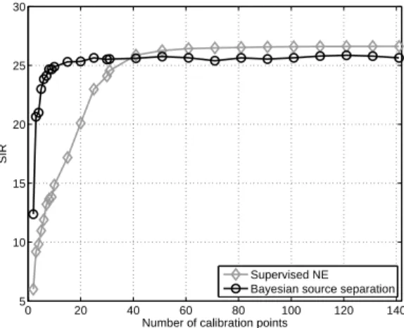
In fact, the argument presented in the last paragraph is some-what naive since it implicitly assumes that the performance of a supervised method does not depend on the number of training samples, which is not the case. Indeed, in Fig. 6, we present the evolution of the training error of the supervised-NE method as the number of calibrations points Ncal grows.
In this figure, which represents an average of 100 runs, one can note that supervised-NE method requires, at least, Ncal=
25 for providing good estimations. Conversely, our proposal requires only Ncal = 5 to provide equivalent estimations8.
This is achieved because the “real” data processing in our
8In Fig. 6, if the test error were plotted, then the difference between the
0 20 40 60 80 100 120 140 5 10 15 20 25
Number of calibration points
SIR
Supervised NE Bayesian source separation
Fig. 6. Performance index as the number of calibration points grows.
proposal is done by the Bayesian BSS algorithm, whereas the calibration points are only used to circumvent the signal ambiguities. Hence, although the complete suppression of the calibration stage is not possible, our method can work even if only a few calibration samples are available.
D. Discussion
The experiments with artificial data attested that the pro-posal can achieve good estimations even in the difficult case where the valences are different. In the scenario with real data, the Bayesian algorithm achieved a much better performance than the ICA-based PNL algorithm. In fact, in this case the sources were clearly dependent and, thus, they violated the fundamental assumption of any ICA method. Evidently, a scenario with dependent sources also poses a problem to a Bayesian method, since there is no guarantee that the provided data representation is unique in such a case. Nonetheless, in contrast to ICA, a Bayesian method does not optimize a functional associated with the statistical independence. Rather, it searches for a “good” data representation given a set of prior information. Thus, in the Bayesian approach, the independence should be seen as a simplifying assumption, that is, we are just omitting an additional prior information to the inference machine, which may still work.
Concerning the algorithm’s convergence, we observed that the Gibbs sampler may get trapped in local minima, thus leading to poor estimations. For the situations with two sources the percentage of poor convergences9 was 3% for artificial data and 7% for the real case; in the case with three sources, this value attained 17%. Although we do not have access to the source, it is still possible to identify a bad solution: we observed that poor convergence usually implies in a significant mismatch between the representation provided by the Bayesian algorithm and the actual array response.
Another important point concerns the execution time of our method. For the experiments with real data, the MCMC algorithm took about10 26s to perform 10000 iterations.
Nev-9These percentages were obtained through a visual inspection after 30
executions.
10The method was implemented in Matlab (Windows XP) and the
simula-tions were performed in a Intel Core 2 duo 3GHz, 2048MB RAM.
ertheless, the algorithm took 380s to perform 50000 iterations in the situation with three sources. This points out a well-known drawback of MCMC-based Bayesian methods: their computational burden can become quite large as the number of sources and samples grows.
Finally, let us make a remark concerning the choice of the priors. In this work, we tried to define priors 1) that ease the resulting inference problem and 2) that, based on the avail-able information, limit the range of the unknown parameters. Evidently, there is no guarantee that our choices are optimum and, as we mentioned before, a large dataset of measurements would permit to refine the priors’ definition. An interesting issue in this context would be to compare the selected priors with alternative models. Because the possibilities are non-exhaustive, we consider a single example where, instead of log-normal priors for the sources, Gamma distributions are considered. This distribution also describes non-negative variables and, moreover, provides a flexible solution as it can model from sparse to almost uniform sources [16].
After applying the solution with the Gamma modeling to process the real data, the obtained performance (average of 30 experiments with Ncal = 4 calibration points) —SIR1 = 22.4 dB and SIR2 = 17.5 dB —was inferior to that of the log-normal prior. Furthermore, unlike the log-normal case, it is not possible to find a conjugate prior in the estimation of the Gamma distribution parameters. Thus, it becomes necessary to incorporate an additional MH algorithm into the Gibbs’ sampler, which increases the algorithm’s complexity and has the inconvenient of requiring the definition of instrumental distributions, which is not an easy task.
V. CONCLUSIONS
In this work, we proposed a Bayesian source separation method for unsupervised quantitative analysis via an ISE array. A MCMC algorithm, the Gibbs sampler, was used in the inference stage. We defined the prior distributions based on informations that are usually available in a chemical sensing problem, such as the non-negativity of the sources. The result-ing separation method did well in different scenarios, includresult-ing in a real problem where the estimation of the activities of ammonium and potassium was desired. The results shown that ISE arrays equipped with blind source separation can operate even if only a reduced number of calibration points is available. This nice feature can pave the way for alternatives to supervised methods. For example, a less demanding calibration step could ease analysis in the field.
Despite the encouraging results, there are still some ques-tions that demand future work. A first one concerns the possibility of increasing the precision of the developed source separation method. Indeed, in our experiments with real data, the remaining small interference would not be acceptable in very-high-precision applications. We believe that a more precise mixing model could increase the estimation quality. In this spirit, a first step is to search for alternatives to the NE model that take into account, for example, dynamics aspects of the interference modeling. Furthermore, it could be equally interesting to develop a Bayesian framework based on
a temporal modeling for the sources, since chemical sources do have a time-structure.
ACKNOWLEDGMENTS
L. T. Duarte thanks the CNPq (Brazil) for funding his PhD research. The authors are grateful to Pierre Temple-Boyer, J´erˆome Launay and Ahmed Benyahia (LAAS-CNRS) for the support in the acquisition of the dataset used in this work. Finally, the authors also would like to thank the anonymous reviewers for their insightful comments.
REFERENCES
[1] L. T. Duarte, C. Jutten, and S. Moussaoui, “Ion-selective electrode array based on a bayesian nonlinear source separation method,” in Proceedings
of the 8th ICA Conference (LNCS), 2009, pp. 662–669.
[2] P. Gr¨undler, Chemical sensors: an introduction for scientists and
engi-neers. Springer, 2007.
[3] P. Fabry and J. Fouletier, Eds., Microcapteurs chimiques et biologiques. Lavoisier, 2003, in French.
[4] E. Bakker and E. Pretsch, “Modern potentiometry,” Angewandte Chemie
International Edition, vol. 46, pp. 5660–5668, 2007.
[5] H. Sakai, S. Iiyama, and K. Toko, “Evaluation of water quality and pollution using multichannel sensors,” Sensons and Actuators B, vol. 66, pp. 25–255, 2000.
[6] U. Oesch, D. Ammann, and W. Simon, “Ion-selective membrane elec-trodes for clinical use,” Clinical Chemistry, vol. 32, pp. 1448–1459, 1986.
[7] O. T. Guenat, S. Generelli, N. F. de Rooij, M. Koudelka-Hep, F. Berthi-aume, and M. L. Yarmush, “Development of an array of ion-selective microelectrodes aimed for the monitoring of extracellular ionic activi-ties,” Analytical Chemistry, vol. 78, pp. 7453–7460, 2006.
[8] Y. G. Vlasov, A. V. Legin, and A. M. Rudnitskaya, “Electronic tongue: chemical sensor systems for analysis of aquatic media,” Russian Journal
of General Chemistry, vol. 78, pp. 2532–2544, 2008.
[9] A. Hyv¨arinen, J. Karhunen, and E. Oja, Independent component analysis. John Wiley & Sons, 2001.
[10] P. Comon and C. Jutten, Eds., S´eparation de sources 1 : concepts
de base et analyse en composantes ind´ependantes. Hermes Science Publications, 2007, in French.
[11] C. Jutten and J. Karhunen, “Advances in blind source separation (BSS) and independent component analysis (ICA) for nonlinear mixtures,”
International Journal of Neural Systems, vol. 14, pp. 267–292, 2004. [12] S. Bermejo, C. Jutten, and J. Cabestany, “ISFET source separation:
foundations and techniques,” Sensors and Actuators B, vol. 113, pp. 222–233, 2006.
[13] G. Bedoya, C. Jutten, S. Bermejo, and J. Cabestany, “Improving semiconductor-based chemical sensor arrays using advanced algorithms for blind source separation,” in Proceedings of Sensors for Industry
Conference, 2004, 2004, pp. 149–154.
[14] L. T. Duarte and C. Jutten, “A mutual information minimization approach for a class of nonlinear recurrent separating systems,” in
Proceedings of the IEEE MLSP 2007, 2007.
[15] C. F´evotte and S. J. Godsill, “A Bayesian approach for blind separation of sparse sources,” IEEE Transactions on Audio, Speech and Language
Processing, vol. 14, pp. 2174–2188, 2006.
[16] S. Moussaoui, D. Brie, A. Mohammad-Djafari, and C. Carteret, “Sepa-ration of non-negative mixture of non-negative sources using a bayesian approach and mcmc sampling,” IEEE Transactions on Signal Processing, vol. 54, pp. 4133–4145, 2006.
[17] C. P. Robert and G. Casela, Monte Carlo Statistical Methods, 2nd ed. Springer, 2004.
[18] C. P. Robert, The Bayesian Choice. Springer, 2007.
[19] Y. Umezawa, P. B¨uhlmann, K. Umezawa, K. Tohda, and S. Amemiya, “Potentiometric selectivity coefficients of ion-selective electrodes,” Pure
and Applied Chemistry, vol. 72, pp. 1851–2082, 2000.
[20] S. A. Dorneanu, V. Coman, I. C. Popescu, and P. Fabry, “Computer-controlled system for ISEs automatic calibration,” Sensons and Actuators
B, vol. 105, p. 521531, 2005.
[21] M. Hartnett and D. Diamond, “Potentometric nonlinear multivariate calibration with genetic algorithm and simplex optmization,” Analytical
Chemistry, vol. 69, pp. 1909–1918, 1997.
[22] A. Doucet and X. Wang, “Monte Carlo methods for signal processing,”
IEEE Signal Processing Magazine, vol. 22, pp. 152–170, 2005. [23] S. M. Kay, Fundamentals of statistical signal processing: estimation
theory. Prentice-Hall, 1993.
[24] L. T. Duarte, R. Suyama, R. R. F. Attux, F. J. V. Zuben, and J. M. T. Romano, “Blind source separation of post-nonlinear mixtures using evolutionary computation and order statistics,” in Proceedings of the
6th ICA Conference (LNCS), 2006, pp. 66–73.
Leonardo Tomazeli Duarte received the B.S and the M.S. degrees in electrical engineering from the University of Campinas (Unicamp), Campinas, Brazil, in 2004 and 2006 respectively. He is currently a PhD student at the Grenoble Institute of Technol-ogy (Grenoble INP), working at the Grenoble im-ages, speech, signal and control laboratory (GIPSA-lab), France. His research interests include blind source separation, independent component analysis, smart chemical sensor arrays and nonlinear models.
Christian Jutten received the PhD degree in 1981 and the Docteur `es Sciences degree in 1987 from the Institut National Polytechnique of Grenoble (France). He taught as associate professor in the Electrical Engineering Department from 1982 to 1989. He was visiting professor in Swiss Federal Polytechnic Institute in Lausanne in 1989, before to become full professor in University Joseph Fourier of Grenoble. He is currently associate director of the Grenoble images, speech, signal and control laboratory (GIPSA, 300 people) and head of the Department Images-Signal (DIS) of this laboratory. For 25 years, his research interests are blind source separation, independent component analysis and learning in neural networks, including theoretical aspects and applications in signal processing (biomedical, seismic, speech). He is author or co-author of more than 45 papers in international journals, 3 books, 16 invited papers and 140 communications in international conferences. He has been associate editor of IEEE Trans. on Circuits and Systems (1994-95), and co-organizer the 1st International Conference on Blind Signal Separation and Independent Component Analysis (Aussois, France, 1999). He has been a scientific advisor for signal and images processing at the French Ministry of Research from 1996 to 1998 and for the French National Research Center from 2003 to 2006. He has been associate editor of IEEE Trans. CAS from 1992 to 1994. He is a member of the technical committee Blind signal Processing of the IEEE CAS society and of the technical committee Machine Learning for signal Processing of the IEEE SP society. He is a reviewer of main international journals (IEEE Trans. on Signal Processing, IEEE Signal Processing Letters, IEEE Trans. on Neural Networks, Signal Processing, Neural Computation, Neurocomputing, etc.) and conferences in signal processing and neural networks (ICASSP, ISCASS, EUSIPCO, etc.). He received the EURASIP best paper award in 1992 and Medal Blondel in 1997 from SEE (French Electrical Engineering society) for his contributions in source separation and independent component analysis, and has been elevated as a Fellow IEEE and a senior Member of Institut Universitaire de France in 2008.
Sa¨ıd Moussaoui received the State engineering de-gree from Ecole Nationale Polytechnique, Algiers, Algeria, in 2001, and the Ph.D. degree in 2005 from Universit Henri Poincar, Nancy, France. He is currently Associate Professor at Ecole Centrale de Nantes. Since september 2006, he is with the Institut de Recherche en Communications et Cybrntiques de Nantes (IRCCYN, UMR CNRS 6597). His research interests are in statistical signal processing methods and their applications.


![[PDF] Cours de base pour apprendre a programmer avec Perl | Cours perl](data:image/gif;base64,R0lGODlhAQABAIAAAP///wAAACH5BAEAAAAALAAAAAABAAEAAAICRAEAOw==)