High-dimensional Bayesian inference via the Unadjusted Langevin Algorithm
Texte intégral
Figure
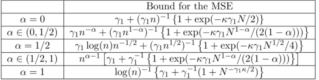
![Table 1: Dependencies of the number of iterations n ε to get W 2 (δ x ⋆ R γ n ε ε , π) ≤ ε For simplicity, consider sequences (γ k ) k≥1 defined for all k ≥ 1 by γ k = γ 1 k −α , for γ 1 < 1/(m + L) and α ∈ (0, 1]](https://thumb-eu.123doks.com/thumbv2/123doknet/8026239.268981/9.892.135.770.162.323/table-dependencies-number-iterations-simplicity-consider-sequences-defined.webp)


Documents relatifs
A sharp affine isoperimetric inequality is established which gives a sharp lower bound for the volume of the polar body.. It is shown that equality occurs in the inequality if and
If q ∈ ∂Ω is an orbit accumulation point, then ∆ ∂Ω q is trivial and hence there does not exist a complex variety on ∂Ω passing through
In Section 6 we obtain explicit lower bounds on this density on bounded sets in the plane in terms of the renormalized energy for a finite number of points.. We are then in
In this note, we prove a sharp lower bound for the log canonical threshold of a plurisubharmonic function ϕ with an isolated singularity at 0 in an open subset of C n.. The
It is essentially a local version of Tian’s invariant, which determines a sufficient condition for the existence of Kähler-Einstein metrics....
Jean-Pierre Demailly / Pha.m Hoàng Hiê.p A sharp lower bound for the log canonical threshold.. log canonical threshold of
We prove that the average complexity, for the uniform distri- bution on complete deterministic automata, of Moore’s state minimiza- tion algorithm is O(n log log n), where n is
If the datagram would violate the state of the tunnel (such as the MTU is greater than the tunnel MTU when Don’t Fragment is set), the router sends an appropriate ICMP
