HAL Id: hal-03105421
https://hal.archives-ouvertes.fr/hal-03105421
Submitted on 23 Mar 2021
HAL is a multi-disciplinary open access
archive for the deposit and dissemination of sci-entific research documents, whether they are pub-lished or not. The documents may come from teaching and research institutions in France or abroad, or from public or private research centers.
L’archive ouverte pluridisciplinaire HAL, est destinée au dépôt et à la diffusion de documents scientifiques de niveau recherche, publiés ou non, émanant des établissements d’enseignement et de recherche français ou étrangers, des laboratoires publics ou privés.
Unraveling spectral shapes of adventitious carbon on
gold using a time-resolved high-resolution X-ray
photoelectron spectroscopy and principal component
analysis
Vincent Fernandez, Neal Fairley, Jonas Baltrusaitis
To cite this version:
Vincent Fernandez, Neal Fairley, Jonas Baltrusaitis. Unraveling spectral shapes of adven-titious carbon on gold using a time-resolved high-resolution X-ray photoelectron spectroscopy and principal component analysis. Applied Surface Science, Elsevier, 2021, 538, pp.148031. �10.1016/j.apsusc.2020.148031�. �hal-03105421�
Applied Surface Science
Unraveling Spectral Shapes of Adventitious Carbon on Gold Using a Time-Resolved
High-Resolution X-ray Photoelectron Spectroscopy and Principal Component Analysis
--Manuscript
Draft--Manuscript Number:
Article Type: Full Length Article
Keywords: X-ray photoelectron spectroscopy; spectral envelope; adventitious carbon; gold; Principal Component Analysis
Corresponding Author: Jonas Baltrusaitis, Ph.D. Lehigh University
Bethlehem, Pennsylvania UNITED STATES
First Author: Vincent fernandez
Order of Authors: Vincent fernandez
Neal Fairley
Jonas Baltrusaitis, Ph.D.
Abstract: To extract chemical information reliably, we propose a new data processing method based both on the creation of information vectors and on a vector base change. The originality of this method is the combination of the different core XPS peaks, Auger and/or valence bands in a single vector. We show that the measurement of a sample upon its progressive chemical change, such as accumulation of the adventitious carbon, allows us to create a new vector basis using linear algebra and Principal Component Analysis. We demonstrate the application of this method using
adventitious carbon films on Au foil utilizing Au 4f, C 1s and O 1s spectral envelopes. This method expands the possibilities of XPS measured chemical environment analysis and is an operator-unbiased solution for materials for which the reference XPS spectra are not available. In this demonstration, the emphasis is placed on identifying changes in a C 1s peak assumed to be adventitious carbon and highlight uncertainties associated with calibrating the binding energy scale using a simple peak model to identify a component C 1s assumed to be saturated hydrocarbon in origin. Suggested Reviewers: Mark Biesinger
biesingr@uwo.ca David Morgan morgandj3@cardiff.ac.uk David Scanlon d.scanlon@ucl.ac.uk Josh Lipton-Duffin josh.liptonduffin@qut.edu.au
1
Unraveling Spectral Shapes of Adventitious Carbon on Gold Using a Time-Resolved High-Resolution X-ray Photoelectron Spectroscopy and Principal Component Analysis
Vincent Fernandez,1 Neal Fairley2 and Jonas Baltrusaitis,3,*
1Institut des Matériaux Jean Rouxel, 2 rue de la Houssinière, BP 32229, F-44322 Nantes Cedex 3, France
2Casa Software Ltd, Bay House, 5 Grosvenor Terrace, Teignmouth, Devon TQ14 8NE, UK 3Department of Chemical and Biomolecular Engineering, Lehigh University, 111 Research Drive,
Bethlehem, PA 18015, USA
Abstract
To extract chemical information reliably, we propose a new data processing method based both on the creation of information vectors and on a vector base change. The originality of this method is the combination of the different core XPS peaks, Auger and/or valence bands in a single vector. We show that the measurement of a sample upon its progressive chemical change, such as accumulation of the adventitious carbon, allows us to create a new vector basis using linear algebra and Principal Component Analysis. We demonstrate the application of this method using adventitious carbon films on Au foil utilizing Au 4f, C 1s and O 1s spectral envelopes. This method expands the possibilities of XPS measured chemical environment analysis and is an operator-unbiased solution for materials for which the reference XPS spectra are not available. In this demonstration, the emphasis is placed on identifying changes in a C 1s peak assumed to be adventitious carbon and highlight uncertainties associated with calibrating the binding energy scale using a simple peak model to identify a component C 1s assumed to be saturated hydrocarbon in origin.
*corresponding author: job314@lehigh.edu; +1-610-758-6836
keywords: X-ray photoelectron spectroscopy; spectral envelope; adventitious carbon, gold, Principal Component Analysis
2 Introduction
X-ray Photoelectron Spectroscopy (XPS) is frequently utilized to provide a chemical interpretation of certain material surface properties [1]. The materials analyzed range from complex inorganic or biological materials under UHV conditions while also excelling in the reactive environments at the pressures approaching those of atmospheric [1–4]. A particularly powerful feature of XPS is the response of the photoelectron transition to the chemical environment resulting in shifts in binding energy for the observed peaks [5]. While different chemical environments result in the corresponding recorded binding energy peak shifts, a binding energy scale for XPS is seldom absolute and it is common to see energy calibration relative to a C 1s peak assumed to be a saturated carbon source, where the binding energy is typically assigned a value of 284.9 eV [6]. The shortcomings of this very popular energy calibration approach have been extensively described in the literature over several decades [6,7] yet it remains arguably the most easily implementable and used approach. The shortcomings include the fact that there are variations in the C 1s binding energy of the adventitious hydrocarbon contamination layer concerning the substrate on which it was measured as well as the source of the adventitious layers. Furthermore, electronic effects such as the alignment with the vacuum level can result in a significant spread when utilizing C 1s binding energy for calibration [8]. On the other hand, standard gold (Au) thin film samples are readily available and are often used as part of intensity calibration procedures [9]. Indeed, intensity calibration is typically performed by repeatedly measuring the same Au sample using different operating modes for an instrument to estimate the intensity response of an instrument to electron emission over a range of kinetic energies and operating modes. A key feature of an intensity calibration procedure is the Au sample must periodically be cleaned by ion gun sputtering to prevent the build-up of carbon contamination within the vacuum chamber. In the absence of cleaning cycles with an ion gun, the spectra typically show steadily increasing C 1s peak. Any overlayer build up alters the shape of the background in an Au spectrum which is an issue for transmission correction. However, a problem for intensity calibration becomes an advantage for the current investigation as it suggests the C 1s peak will alter with time due to deposition from the vacuum chamber. Chemistry of Au as measured by XPS is rather simple so the C 1s peak is expected to alter only in terms of carbon bonded to oxygen and hydrogen. The inert nature of Au suggests the Au 4f doublet is well defined and does not change as a consequence of changes in carbon chemistry. Spectra for Au 4f,
3
therefore, provide a very stable reference in terms of binding energy, albeit rarely used experimentally in a routine XPS work. Further, Au does not require charge compensation in the form of a source of charged particles required by a non-conducting material to maintain a constant potential at the surface, thus the sample and measurement process is well understood.
In this work, the common practice of calibrating XPS spectra in terms of binding energy based on adventitious carbon C 1s peak is examined by considering a standard Au sample exposed to the atmosphere. The initial surface after repeated measurement within an XPS instrument yields C 1s spectra with clear evidence of evolution in terms of spectral shape as a function of time. These spectra are analyzed using newly developed methods based on linear analysis and nonlinear optimization. The objective is to identify changes in a C 1s peak assumed to be adventitious carbon and highlight uncertainties associated with calibrating the binding energy scale using a simple peak model to identify a component C 1s assumed to be saturated hydrocarbon in origin, in line with recent developments of the XPS data processing methods that minimize user bias [10,11]. This analysis is done to highlight the coarse nature of this approach to binding energy calibration and to illustrate how the binding energy scale so defined can alter simply due to the influences of time on a sample when placed in a vacuum.
Experimental
Spectra were acquired from a Kratos Axis Ultra using the same physical position on an Au sample previously used as a standard material for intensity calibration of said XPS instrument. The Au sample received no special treatment but was introduced to vacuum with residual contamination typical of a sample stored in a laboratory. Data were measured using hybrid mode as defined by Kratos Analytical Limited using slot aperture and pass energy 20 eV. No charge neutralization was performed. Rather, the sample was grounded to maintain a constant surface potential which was verified by the stability of the Au 4f doublet binding energy peak position and uniform shape throughout all measurement cycles.
The set of spectra measured during a measurement cycle include a survey spectrum and high-resolution spectra acquired over energy intervals for Au 4p3/2 in addition to O 1s, C 1s, Au 4f and valence band data. Each acquisition cycle elapsed time was 102 minutes. The experiment consisted of 31 acquisition cycles measured over two days.
4 Spectral Data Analysis
All results were processed using CasaXPS software. Analysis of these data was focused chiefly on the C 1s peak intensities. However, to assist the procedure, intensities for C 1s, O 1s and Au 4f were organized to form a single vector as shown in Figure 1 using the procedure described below. Although changes as a result of the measurement process were most obvious in the C 1s data, utilizing the O 1s and Au 4f data prevented the selection of non-physical data transformations since a transformation to the C 1s intensities must also yield meaningful shapes for the O 1s and Au 4f data. It should be noted that the only function of including the Au 4f doublet is to provide a stable energy reference for these transformations. That is, no transformation should yield a significant deformation of the Au 4f intensities compared to the initial doublet peaks.
The basis for data treatment performed herein is the application of linear algebra to vectors formed from spectra [12]. The objective is to create a set of spectral forms, not necessarily measured spectra but rather derived from measured spectra, that can be used to fit the original spectra in a traditional linear least-squares approach. The assumption was that these derived spectral forms are vectors that can be interpreted with a physical meaning.
When presented with a set of evolving data vectors the first task is to assess the number of spectral shapes that are required to permit a linear least-squares approximation to data that offers data reproduction consistent with Poisson distributed signal [13]. A technique for making such an assessment is principal component analysis (PCA), which is a procedure for transforming data vectors to abstract data vectors referred to as abstract factors (AFs) [14]. The number of AFs for which variation about zero is greater than noise expected for pulse counted data provides a measure for the number of spectral forms required to reproduce the original data with the appropriate precision [14]. An understanding of PCA is therefore integral to computing physically meaningful spectral forms.
Arguably the best way to appreciate the meaning for a PCA AF is to consider the construction of three AFs calculated from three data vectors. In mathematical terms, a PCA makes use of the following matrix definitions.
5
Given a set of three data vectors {𝒅1, 𝒅2, 𝒅3}, the standard procedure for expressing these three vectors as a corresponding set of abstract vectors {𝒖1, 𝒖2, 𝒖3} is in terms of a singular value decomposition (SVD) [12]
𝑫 = 𝑼𝑾𝑽𝑇 (1),
where 𝒅𝑖 ∈ ℝ𝑛, 𝒖
𝑖 ∈ ℝ𝑛, 𝑫 = [𝒅1, 𝒅2, 𝒅3] and 𝑼 = [𝒖̂1, 𝒖̂2, 𝒖̂3] (2) 𝑾 is a diagonal matrix with diagonal matrix elements equal to the square root of the eigenvalues computed for the covariance matrix
𝒁 = 𝑫𝑇𝑫 (3)
and 𝑽 is the matrix formed from the normalized eigenvectors of 𝒁 ordered with respect to the eigenvalues. These values appear ordered by size along the diagonal of 𝑾.
The output from a PCA calculation applied to three data vectors is three abstract vectors with the characteristics of these data vectors. These outputs from PCA are the desired AFs. The relationship between these three abstract factors and the original data vectors can be understood by considering a distribution of points in a 3D space. These points in a 3D space are formed by allocating from each data vector one coordinate and making use of a specific coordinate from each data vector to specify the three coordinates for a point in 3D space. Plotting these points in 3D results in a distribution of points and the first abstract factor, in a PCA approach, is formed from a 3D position vector that minimizes the sum of square perpendicular distances from each point in the distribution to the position vector. By definition, the position vector with these properties can be used to compute a vector with the dimensions of a data vector that is most representative of all three data vectors. Applying calculus to minimize the sum of square perpendicular distances subject to the constraint that the position vector is not the zero vector leads to formulating the eigenproblem the solution of which yields the two matrices 𝑽 and 𝑾
[ 𝒅1. 𝒅1 𝒅1. 𝒅2 𝒅1. 𝒅3 𝒅1. 𝒅2 𝒅2. 𝒅2 𝒅2. 𝒅3 𝒅1. 𝒅3 𝒅2. 𝒅3 𝒅3. 𝒅3] [ 𝛼 𝛽 𝛾] = 𝜆 [ 𝛼 𝛽 𝛾] (4).
6
𝑼 = 𝑫𝑽𝑾−𝟏 (5).
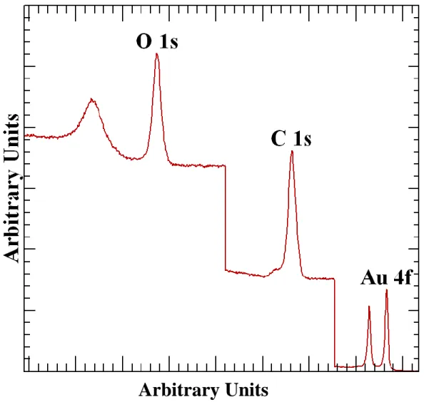
The concept of position vectors in 3D can be generalized to an m-dimensional space and the mathematical analysis leading to the need for the solution of an m x m real symmetric matrix also generalizes from 3-dimensions to m-dimensions. The data set used throughout this paper requires the formation of a 31-dimensional eigenproblem corresponding to 31 vectors constructed from 31 experiment cycles including measurement of O 1s, C 1s and Au 4f narrow scan spectra. When these three spectra are combined as seen in Figure 1 the total number of data channels is 845, therefore the dimension for the data vectors is 845 but these vectors can span at most a subspace of dimension 31.
The algorithm used to compute eigenvectors and eigenvalues is iterative SVD [15]. Iterative SVD permits a limited number of eigenvectors and eigenvalues to be determined, thus targeting computation time to abstract vectors of importance to a given data set. From the perspective of the 31 vectors used here, computation time is not significant but for larger problems, iterative SVD presents a tool for saving time without compromising numerical precision.
Results and Discussion
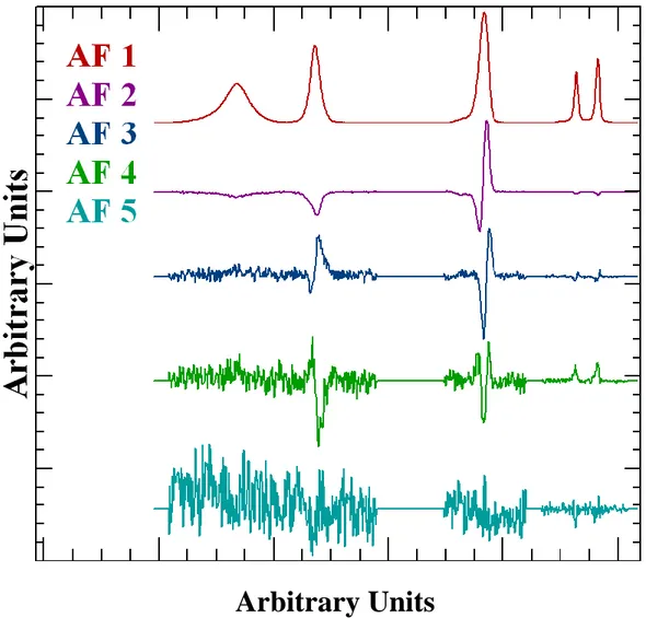
We begin the analysis by defining a set of 31 vectors corresponding to each measurement cycle equivalent to the data in Figure 1 which are assessed in terms of a PCA. The objective of performing the PCA is to establish how many different shapes are required to describe the data set as a whole. The role of a PCA is to transform these initial vectors into a set of vectors containing the same shape information as the original set of vectors.
Mathematical procedures for computing PCA abstract factors, the first five of which are shown overlaid in Figure 2, represent recipes for collecting information of significance into as few vectors as necessary capable of describing the vector space spanned by the vectors in their original form. In principle, each of the original vectors can be reconstructed from these abstract factors by an optimization routine using these abstract factors as lineshapes. Here the term lineshape is used in a loose sense of the word as abstract factors shown in Figure 2 include shapes unknown in terms of XPS peaks. Nevertheless, by summing in the correct proportions of these abstract factors, each spectrum in the original data set can be reproduced to a precision only limited by the number of abstract factors used in the optimization procedure as lineshapes. Selecting the abstract factors in
7
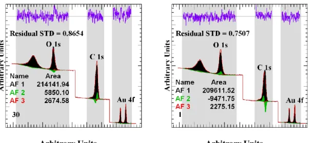
the order shown in Figure 2 suggest a good reproduction will be achieved by using only the first three most significant abstract factors. The conclusion from the PCA is, therefore, the original vectors contain three trends that manifest as these abstract factors. The current approach requires sets of data with only two trends. Hence the data set must be sub-sampled in an attempt to simplify the analysis. The challenge is to partition the original data set into subsets for which only two abstract factors are identified by PCA and then manipulate the subset using vector subtraction to yield shapes more representative of real physical peaks found in spectra. The ultimate goal is to manipulate these subsets to uncover three physically meaningful spectral shapes which when used as lineshapes can reproduce the entire data set. The abstract factors are plotted using different scale factors to emphasize shape information in these vectors. Figure 2, therefore, exaggerates the significance of these abstract factors concerning the original data set. Figure 3 illustrates two spectra fitted using the first three abstract factors. The non-physical nature of these abstract factors is evident in Figure 3, where it can be seen a fit is achieved for these two examples by reversing the direction of the second abstract factor. It can also be seen in Figure 3 that these abstract factors do not obey the normal convention for component spectra which require positive peak area parameters, but the sign for the magnitude of the second abstract factor switches when fitting these two data envelopes. As a consequence, the first abstract factor can include intensities greater than the spectral intensities. The conclusion is these abstract factors are purely mathematical.
Abstract factors by their very nature are not physically significant. The least-squares principle applied to the logic described above provides one useful physical interpretation, namely, the first abstract factor is a sophisticated averaging of data vectors hence for spectroscopic data formed from photoemission peaks the first abstract factor has the characteristics of bell-shaped curves superimposed on background signal. However, the abstract factors in Figure 2 are computed from spectroscopic data pre-processed to remove the inelastically scattered background using a Tougaard approach [16,17]. For this reason, the first abstract factor has the appearance of bell-shaped curves only. Subsequent abstract factors for the calculation resulting in Figure 2 show features that can be associated with the location of peaks, but resemble derivatives of peaks rather than peaks as such. Removing background from data before computing abstract factors allows the use of these abstract factors in Figure 2 in peak models shown in Figure 3 which are fitted to data using non-linear optimization. Three abstract factors are selected from the computed abstract factors and the act of fitting these three abstract factors to data vectors is the equivalent of forming
8
a linear combination of these three abstract factors where the linear coefficients are determined in a linear least-squares approach. The results are shown in Figure 3 demonstrate for these data vectors that fitting the first three abstract factors to these data vectors results in data reproduction with a residual standard deviation of the magnitude expected for pulse counted data compiled from multiple data streams. The act of fitting these data using three abstract factors as component line shapes demonstrates these data vectors all lie in a 3-dimensional subspace and that differences between these 31 data vectors and a linear least-squares approximation formed from three linearly independent vectors spanning the same subspace as the first three abstract factors are no greater than would be expected for variations due to Poisson distributed signal. The implication of this statement is the problem of separating spectroscopic information into physically significant shapes is that of identifying three spectroscopic shapes that are linearly independent.
From a mathematical perspective, subtracting a background representing an inelastically scattered signal represents a transformation applied to the original data. PCA calculations can be performed directly on data, however, it is also common practice to perform data scaling [18] as a means of reducing the influence of noise on abstract factors to promote information content in the most significant abstract factors. Another common practice is to mean center data vectors, which in mathematical terms changes the origin for the data vectors before computing abstract factors. Removing background signal from data vectors is analogous to mean centering the data vectors but retains essentially spectroscopic recognizable forms within data vectors used in the PCA calculation. Subtracting a background or subtracting a mean spectrum from data vectors are both numerically advantageous as both reduce the loss of significant digits when computing the eigenvalues and eigenvectors. The advantage of applying PCA to data vectors after removal of background signal is that the relationship between abstract factors and the original data vectors can be demonstrated as shown in Figure 3 and that fitting of abstract factors to data requires abstract factors that are not physically meaningful. Fitting of these same data vectors with physically meaningful components with shapes comparable with bell-shaped curves requires linearly independent spectral shapes that are not necessarily orthogonal.
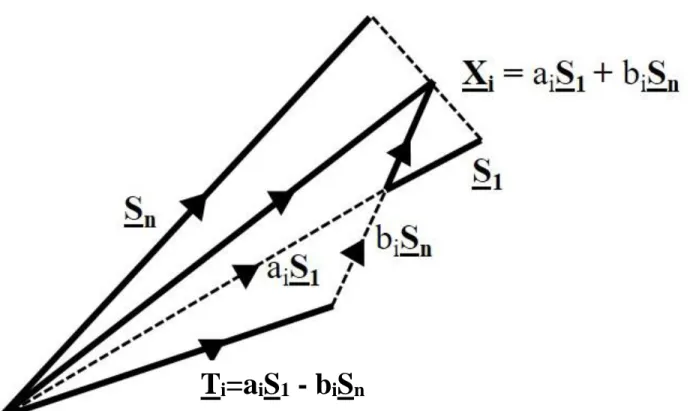
The approach used to analyze these 31 data vectors is based on manipulating spectra two at a time to create three linearly independent component vectors with characteristics of spectral forms that retain physically meaningful interpretation. Data vectors are transformed by the construction
9
shown in Figure 4, the outcome of which is illustrated in Figure 5, left. In essence, two data vectors are selected from the set of 31 data vectors. Then by considering the difference vector formed from these two data vectors S1 and Sn a new vector Ti is selected as an interim spectral form. The chosen vector Ti may need further adjustments en route to deriving three-component vectors with characteristics of spectral forms belonging to the same subspace as the three most significant abstract factors equivalent to the abstract factors shown in Figure 2. The calculation in Figure 5, left differs from the results in Figure 2 in that in Figure 5, left data vectors are used without pre-processing of data vectors to remove background influences.
An example of an analysis based on the transformation steps described in Figure 4 is shown in Figure 5, right. The C 1s data envelope is decomposed into three components, namely C 1s a, C 1s b and C 1s c while the data treatment retains features typical of Au 4f and O 1s spectra in computed components. It is thought unlikely that carbon is chemically linked to Au, so the existence of gold peaks in these components is logically equivalent to measuring these forms of carbon on a gold substrate. Hence, the analysis partitions the C 1s region into three chemically shifted forms. One form, C 1s b, with characteristics expected for carbon bonded to oxygen at 286.5 eV includes minor C 1s peaks possibly C-H (285) and C=O or C-O-C (288-290 eV) [19,20]. This can be proposed as the initial adventitious carbon state. On the other hand, the C 1s a form which, when applied to the data in the current experiment, monotonically increases with measurement time and is thought to be C-C or C-H type chemistry analogous to PMMA type of H2C-C-C=O bond with the peak at 285.72 eV and C-H3 at 285 eV[20], which are summed to form a single trace in Figure 6, e.g. C 1s a c. The quantification in Figure 6 of these data is performed using Kratos relative transmission correction using Kratos relative sensitivity factors (RSFs) that assume elements appear as bulk materials within the sampling depth for photoemission due to scattering of photons with energy 1486.6 eV. Since carbon is shown to be a surface layer using cleaning the sample with an ion beam, the percentage of carbon is amplified relative to gold by the use of bulk RSFs and further amplified by attenuation of a substrate material relative to an overlayer of carbon. It can be, therefore, concluded that carbon is present in significant proportions but is not as significant as the profile would suggest. Nevertheless, changes in carbon are the dominant process during these measurement cycles and forming an interpretation for these carbon components shown in Figure 5 is appropriate for these data.
10
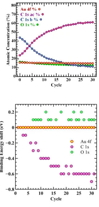
The trend plot in Figure 6 shows how a gold sample with an overlayer of adventitious organic material is modified over an extended period under analysis conditions. The most significant change to the surface is observed in the C 1s intensities where the peak maximum shifts by 0.6 eV throughout the experiment relative to a very stable position for the Au 4f peaks. This peak shift of 0.6 eV is a consequence of an alteration in carbon chemistry caused by an increasing quantity of C-C and C-H type bonds as defined above in addition to and at the expense of C-O type bonds resulting in a movement to lower binding energy, with time, for the C 1s peak maximum. The analysis shows the C 1s data envelope is heavily influenced by two peak envelopes (C-O and combined C-C/C-H) separated by 0.82 eV and the varying proportions for these two sources of carbon cause the shift in peak maximum.
Highly correlated peak structures, such as the ones shown in Figure 5, are difficult to analyze with conventional synthetic components constructed from Voigt like functional forms and without significant levels of fitting-parameter constraints. Determining a consistent peak position for these carbon peaks is prone to error. It is therefore clear from these measurements an energy calibration based on the C 1s spectra would rely on knowledge of the sample history and while the chemistry of adventitious carbon is typically of no interest to most samples upon which XPS is performed, the use of adventitious carbon as a means of calibrating the binding energy scale is of some importance, particularly if binding energy assignments for peaks of interest are of significance to an XPS analysis.
Conclusions
By examining the evolution of C 1s spectra measured from a gold sample with normal adventitious contamination, the extent to which C 1s can be used as a binding energy reference is assessed. A technique for extracting lineshapes based on data is described and conclusions based on these measurements suggest precise binding energy calibration requires a careful analysis of a C 1s peak structure resulting from unknown surface contaminants. Routine use of binding energy calibration based on identifying the saturated carbon peak is deemed to be only a rough approximation and unsuitable as a means of locating a peak of interest in terms of precise binding energy.
The XPS data analysis often does not fall into a category of rigorous analysis but is reliant on the user’s ability to guide these transformations to a plausible solution. Solutions must be tested
11
against the data set to ensure data reproduction can be achieved and sample knowledge is used to discriminate against poor conclusions. The advantage of the approach described is that component shapes are derived from data rather than assuming mathematical shapes for underlying peaks. Indeed, the need to identify every underlying component peak is not required by the current approach, but partial decomposition into components provides insight into the structure in terms of traditional component peaks not obvious from the initial data set.
Acknowledgments. This work by J.B. was supported as part of UNCAGE-ME, an Energy Frontier Research Center funded by the U.S. Department of Energy, Office of Science, Basic Energy Sciences under Award No. DE-SC0012577.
12 References
[1] D.R. Baer, M.H. Engelhard, XPS analysis of nanostructured materials and biological surfaces, J. Electron Spectros. Relat. Phenomena. 178–179 (2010) 415–432.
https://doi.org/10.1016/j.elspec.2009.09.003.
[2] A.R. Head, H. Bluhm, Ambient Pressure X-Ray Photoelectron Spectroscopy, in: K.B.T.-E. of I.C. Wandelt (Ed.), Ref. Modul. Chem. Mol. Sci. Chem. Eng., Elsevier, Oxford, 2016: pp. 13–27. https://doi.org/10.1016/B978-0-12-409547-2.10924-2.
[3] M. Salmeron, From Surfaces to Interfaces: Ambient Pressure XPS and Beyond, Top. Catal. 61 (2018) 2044–2051. https://doi.org/10.1007/s11244-018-1069-0.
[4] M. Salmeron, R. Schlogl, Ambient pressure photoelectron spectroscopy: A new tool for surface science and nanotechnology, Surf. Sci. Rep. 63 (2008) 169–199.
https://doi.org/10.1016/j.surfrep.2008.01.001.
[5] M. Descostes, F. Mercier, N. Thromat, C. Beaucaire, M. Gautier-Soyer, Use of XPS in the determination of chemical environment and oxidation state of iron and sulfur samples: constitution of a data basis in binding energies for Fe and S reference compounds and applications to the evidence of surface species of an oxidized py, Appl. Surf. Sci. 165 (2000) 288–302. https://doi.org/10.1016/S0169-4332(00)00443-8.
[6] G. Greczynski, L. Hultman, X-ray photoelectron spectroscopy: Towards reliable binding energy referencing, Prog. Mater. Sci. 107 (2020) 100591.
https://doi.org/10.1016/j.pmatsci.2019.100591.
[7] P. Swift, Adventitious carbon: the panacea for energy referencing?, Surf. Interface Anal. 4 (1982) 47–51. https://doi.org/10.1002/sia.740040204.
[8] G. Greczynski, L. Hultman, C 1s Peak of Adventitious Carbon Aligns to the Vacuum Level: Dire Consequences for Material’s Bonding Assignment by Photoelectron Spectroscopy, ChemPhysChem. 18 (2017) 1507–1512. https://doi.org/10.1002/cphc.201700126. [9] G. Hopfengärtner, D. Borgmann, I. Rademacher, G. Wedler, E. Hums, G.W. Spitznagel,
13
Electron Spectros. Relat. Phenomena. 63 (1993) 91–116. https://doi.org/10.1016/0368-2048(93)80042-K.
[10] J. Baltrusaitis, B. Mendoza-Sanchez, V. Fernandez, R. Veenstra, N. Dukstiene, A. Roberts, N. Fairley, Generalized molybdenum oxide surface chemical state XPS determination via informed amorphous sample model, Appl. Surf. Sci. 326 (2015) 151–161.
https://doi.org/10.1016/j.apsusc.2014.11.077.
[11] V. Fernandez, D. Kiani, N. Fairley, F.-X. Felpin, J. Baltrusaitis, Curve fitting complex X-ray photoelectron spectra of graphite-supported copper nanoparticles using informed line shapes, Appl. Surf. Sci. 505 (2020) 143841. https://doi.org/10.1016/j.apsusc.2019.143841. [12] F.L. Bauer, A.S. Householder, J.H. Wilkinson, C. Reinsch, Handbook for Automatic
Computation: Volume II: Linear Algebra, Springer, Berlin Heidelberg, 2012. [13] N. Fairley, CasaXPS French Cookbook: Analysis of Non-Trivial XPS Using Novel
Methodologies: A Companion Text to Videos and Data, Casa Software Ltd, 2014. [14] E.R. Malinowski, Factor analysis in chemistry, 3rd ed., John Wiley & Sons, Ltd, 2002. [15] S. Béchu, M. Richard-Plouet, V. Fernandez, J. Walton, N. Fairley, Developments in
numerical treatments for large data sets of XPS images, Surf. Interface Anal. 48 (2016) 301–309. https://doi.org/10.1002/sia.5970.
[16] S. Tougaard, Quantitative analysis of the inelastic background in surface electron spectroscopy, Surf. Interface Anal. 11 (1988) 453–472.
https://doi.org/10.1002/sia.740110902.
[17] S. Tougaard, Practical algorithm for background subtraction, Surf. Sci. 216 (1989) 343–360. https://doi.org/10.1016/0039-6028(89)90380-4.
[18] J. Walton, N. Fairley, XPS spectromicroscopy: exploiting the relationship between images and spectra, Surf. Interface Anal. 40 (2008) 478–481. https://doi.org/10.1002/sia.2731. [19] D. Briggs, G. Beamson, Primary and secondary oxygen-induced C1s binding energy shifts
14 https://doi.org/10.1021/ac00039a018.
[20] G. Beamson, D. Briggs, High Resolution XPS of Organic Polymers: The Scienta ESCA300 Database, Wiley; 1st edition, 1992.
15
Arbitrary Units
Figure 1: Example of concatenated spectral intensities. The O 1s intensities are maintained at the binding energy for the oxygen transition. C 1s and Au 4f intensities are added to the vector by applying an offset in energy to the true binding energies for these transitions. For the manipulation in vector space results are presented in arbitrary units.
16
Arbitrary Units
Figure 2: PCA decomposition of data set consisting of all 31 vectors. These traces represent the first five abstract factors in which the PCA is collecting shape information into alternative vectors based on a least-squares criterion. These are non-physical in terms of spectroscopy, but mathematically these abstract factors contain the same spectroscopic information as the original spectra.
17
Arbitrary Units Arbitrary Units
18
Figure 4: S1 and Sn are two spectra selected from a range of spectra in an evolving data set such that PCA applied to { S1 … Sn} yield only two abstract factors. The set of vectors Xi=ciS1 + (1-ci)Sn or as an alternative Xi = Si are fitted with lineshapes derived from S1 and Sn and by definition provided a range of fits with various proportions in the two spectra S1 and Sn. A transformed spectrum is chosen from the set of Ti is obtained by selecting an appropriately shaped vector consistent with spectroscopic shapes.
19 Arbitrary Units
Figure 5: (left) An example of a vector Ti constructed from two lineshapes derived from data. The new vector is selected based on the movement to lower binding energy compared to the original spectra S1 and Sn while maintaining appropriate peak shapes for both the O 1s peak and also the well-defined reference shape from the Au 4f doublet. (right): Three vectors constructed (C 1s a, C 1s b and C 1s c) using the procedure described in Figure 4 for a peak model that is fitted to a data vector. The procedure creates new vectors with a clear separation of phases in the carbon data envelope.
20
Figure 6: (top) Examples of C 1s peaks fitted using the component shapes calculated from the data set. It is clear from these C 1s spectra sampled from the data set how differing amounts of these two components account for the shift in peak position. (bottom): Shift of the peak positions as measured by maximum height above a linear background calculated from regions defined on the O 1s, C 1s and Au 4f high-resolution spectra. These energies are calculated directly from the data as acquired without any energy calibration shifts being applied. Note how the C 1s data envelope shifts by ~0.6 eV throughout the measurement while there is no shift for the Au 4f.
Declaration of interests
☒The authors declare that they have no known competing financial interests or personal relationships that could have appeared to influence the work reported in this paper.
☐The authors declare the following financial interests/personal relationships which may be considered as potential competing interests: