HAL Id: hal-00512377
https://hal.archives-ouvertes.fr/hal-00512377
Submitted on 30 Aug 2010HAL is a multi-disciplinary open access archive for the deposit and dissemination of sci-entific research documents, whether they are pub-lished or not. The documents may come from teaching and research institutions in France or abroad, or from public or private research centers.
L’archive ouverte pluridisciplinaire HAL, est destinée au dépôt et à la diffusion de documents scientifiques de niveau recherche, publiés ou non, émanant des établissements d’enseignement et de recherche français ou étrangers, des laboratoires publics ou privés.
FICS 2010
Dale Miller, Arnaud Carayol, Panos Rondogiannis, Lars Birkedal, Marek
Czarnecki, Hervé Grall, Paul Levy, Matteo Mio, Keiko Nakata, Andrei
Romashchenko, et al.
To cite this version:
Dale Miller, Arnaud Carayol, Panos Rondogiannis, Lars Birkedal, Marek Czarnecki, et al.. FICS 2010. 7th Workshop on Fixed Points in Computer Science, FICS 2010, Aug 2010, Brno, Czech Republic. pp.89. �hal-00512377�
FICS 2010, the 7th Workshop on Fixed Points in Computer Science, was held in Brno, Czech Re-public, on August 21-22 2010, as a satellite workshop to the conferences Mathematical Foundations of Computer Science and Computer Science Logic 2010. FICS aims to provide a forum for researchers to present their results to those members of the computer science and logic communities who study or apply the theory of fixed points.
The editor wishes to thank the authors that primarily contributed with their ideas and work to the success of the workshop. He would also like to thank the the external reviewers, Dietmar Berwanger, Mart´ın Escard´o, Martin Lange, Richard McKinley, Dieter Probst, Joshua Sack, and the members of the Program Committee, Thorsten Altenkirch, Giovanna d’Agostino, Peter Dybjer, Zolt´an ´Esik, Anna Ing´olfsd´ottir, Gerhard J¨ager, Ralph Matthes, Andrzej Murawski, Damian Niwinski, Luigi Santocanale, Alex Simpson, Jean-Marc Talbot, Tarmo Uustalu, Yde Venema, Igor Walukiewicz, for their collaboration in the process of selecting the contributions. Finally, the editor wishes to thank Tony Kuˇcera and Tom´aˇs Br´azdil for taking care of the local organization of the workshop.
A special thank goes to the French institutions that made the organisation of the workshop possible through their financial support:
- Laboratoire d’Informatique Fondamentale de Marseille (LIF, UMR 6166), - Universit´e Aix-Marseille I (Universit´e de Provence),
- Agence Nationale de la Recherche,
through the projects ECSPER (ANR-JC09-472677) and SFINCS (ANR- 07-SESU-012).
Brno, August 21, 2010, Luigi Santocanale
Invited Talks Arnaud Carayol,
Structures Defined by Higher-Order Recursion Schemes . . . 7 Dale Miller,
Fixed Points and Proof Theory: An Extended Abstract . . . 9 Panos Rondogiannis,
Fixed-Point Semantics for Non-Monotonic Formalisms . . . 17
Contributed Talks
Lars Birkedal, Jan Schwinghammer, Kristian Støvring,
A Metric Model of Lambda Calculus with Guarded Recursion . . . 19 Lars Birkedal, Jan Schwinghammer, Kristian Støvring,
A Step-indexed Kripke Model of Hidden State
via Recursive Properties on Recursively Defined Metric Spaces . . . 27 Marek Czarnecki,
How Fast Can the Fixpoints in Modalµ-Calculus Be Reached? . . . 35 Herv´e Grall,
Proving Fixed Points . . . 41 Paul Blain Levy,
Characterizing Recursive Programs up to Bisimilarity . . . 47 Matteo Mio,
The Equivalence of Game and Denotational Semantics for the Probabilisticµ-Calculus . . . 53 Keiko Nakata,
Denotational Semantics for Lazy Initialization of Letrec . . . 61 Andrei Romashchenko,
Fixed Point Argument and Tilings without Long Range Order . . . 69 Tarmo Uustalu,
A Note on Strong Dinaturality, Initial Algebras
and Uniform Parameterized Fixpoint Operators . . . 77 Paweł Waszkiewicz,
Common Patterns for Metric and Ordered Fixed Point Theorems . . . 83
LIGM
Universit´e Paris-Est and CNRS 5, boulevard Descartes, Champs-sur-Marne
F-77454 Marne-la-Vall´ee Cedex 2 [email protected]
Higher-order recursion schemes are a particular form of typed term rewriting systems. By iterative rewriting from a fixed finite term, an (higher-order) recursion scheme generates at the limit an infinite term. In 2006, Luke Ong has shown that for the infinite terms obtained in this way monadic second-order logic (MSO) is decidable. As terms defined by recursion schemes encompass most of the known examples of infinite terms having decidable MSO theory, this result has revived the interest for recursion schemes.
In this talk, we will survey results concerning the structures defined by recursion schemes. These structures are essentially graphs which can be defined using MSO logic on the terms generated by recur-sion schemes. Our main focus will be to assess the expressivity of these structures through alternative characterisations.
An extended abstract
Dale Miller
INRIA Saclay & LIX/Ecole Polytechnique, Palaiseau, France
Abstract
We overview some recent results in the proof theory for fixed points and illustrate how those re-sults can be used to provide a unified approach to computation, model checking, and theorem proving. A key theme in this work is the development of focused proof system that allow for micro-rules (e.g., sequent calculus introduction rules) to be organized into macro-rules. Such macro-rules can often be designed to correspond closely to “steps” or “actions” taken within computational systems.
1 Introduction
Potentially unbounded behavior is available in proof theory via the contraction rule (see Figure1): when reading this rule from its conclusion to its premise, a formula is duplicated and such duplication can be applied again and again. When contraction is removed, decidability often follows. For example, the multiplicative-additive fragment of linear logic (MALL) does not have contraction (nor weakening) and, as a result, it is decidable whether or not a formula is a theorem. It is possible to given a proof system for propositional intuitionistic logic that does not contain contraction [9]: a naive implementation of that proof system can be a decision procedure for that logic.
Decidable logics, such as MALL and propositional intuitionistic logic, have rather limited applica-tions. For a logic and proof system to find wide ranging applications in, say, computation and deduction, they must allow for potentially infinite behaviors.
Girard designed linear logic to be the result of extending MALL with the exponentials (!, ?): the proof rules of contraction and weakening are allowed only on formulas marked by such exponentials. In this way, potentially infinite behaviors can be mixed with MALL: linear logic becomes undecidable in this way (even the propositional fragment of linear logic is undecidable [12]).
While the addition of the exponentials to MALL is elegant and powerful, the exponentials are not without problems for those working in computational logic. For example, when using (as we will) fo-cused proof systems, the exponentials can cause focusing phases to terminate. Furthermore, exponentials are not canonical: that is, if one allows a “red” version and a “blue” version of both of ! and ?, it is not possible to prove them equivalent (all other connectives of linear logic are canonical in this sense). While there are interesting uses for such non-canonical exponentials (see, for example, the material on subexponentials in [18]) one would like to have alternative approaches to potentially infinite behavior in proof systems.
Baelde and Miller have proposed another approach to extending MALL with potentially infinite behavior: in particular, they have added the least and greatest fixed points directly to MALL [6,3]. The resulting logic is surprisingly elegant and expressive: it has been used to describe the logical foundations of a model checker [5] and is being used to design a new theorem proving architecture for the search for proofs involving induction [7]. The development of a focused proof system for MALL plus fixed points has lead to some new proof theory phenomena as well as some new ways to approach the unity of such different topics as computation, model checking, and inductive and co-inductive theorem proving.
This extended abstract will illustrate some of the proof theory of fixed points by concentrating on adding fixed points to classical first-order logic. Parts of this abstract are based on similar material found in [14].
Fixed points and proof theory: An extended abstract Miller
Structural rules: ` B,B,∆` B,∆ contract ` B,∆` ∆ weaken
Identity rules: ` B,B⊥ initial
` ∆1,B ` B⊥,∆2 ` ∆1,∆2 cut Multiplicative rules: ` B 1,∆1 ` B2,∆2 ` B1∧ B2,∆1,∆2 ∧ ` B1,B2,∆ ` B1∨ B2,∆ ∨ ` t t ` f ,∆` ∆ f Additive rules: ` B 1,∆ ` B2,∆ ` B1∧ B2,∆ ∧ ` Bi,∆ ` B1∨ B2,∆ ∨i ` t,∆ t —
Figure 1: Proof rules for propositional classical logic
2 A focused proof system for classical logic
We now consider propositional classical logic over formulas built from ∧, ∨, t, f . Remarkably, we shall not have a need for atomic formulas. Figure1contains a one-sided sequent calculus proof systems for this logic. A sequent ` ∆ contains a multiset of formulas ∆. Besides containing the usual structural rules and identity rules (initial and cut), the logical connectives have two sets of introduction rules. That is, for each logical connective, there is a set of multiplicative rules and a set of additive rules for it. (The set of additive rules for f is empty and the set of additive rules for ∨ contains two rules.) Notice that the rules for the additive conjunction and the multiplicative disjunction are invertible while the rules for the multiplicative conjunction and the additive disjunction are not necessarily invertible.
The cut rule is admissible and the initial rule is admissible for all but atomic formulas. Since we have no atomic formulas, both identity rules can be dropped.
As is well known, the additive rule and the multiplicative rule for the same connective are inter-admissible in the presence of the structural rules of contraction and weakening. Another way to state this admissibility statement is the following. Annotate names of the connectives in the inference rules as follows: the invertible rules are annotated as negative ∧− and ∨− while the not-necessarily-invertible rules are annotated as positive ∧+ and ∨+ (annotate their units also to be t−, f−, t+, f+). Given a formula B let ˆB be any polarization of B in which every logical connectives in B is given either a plus or a minus annotation. Then, B is provable (in the unannotated proof system) if and only if ˆB is provable (in the annotated proof system). We shall say that an annotated formula is negative if its top-level logical connective is annotated negatively and is positive if its top-level logical connective is annotated positively. By B⊥ we shall mean the negation normal form of B: since we have no atomic formulas, negations will not occur within formulas. Notice that the de Morgan dual of ∨+and ∧+are, respectively, ∧−and ∨−.
If we try to take the construction of proofs literally as a model for performing computation, one is immediately struck by the inappropriateness of sequent calculus rules in Figure1for this task: there are just too many ways to build proofs and most of them differ in truly minor ways. One would like to have a tight correspondence between the application of inference rules and “actions” within a computation. An early attempt to provide the sequent calculus with normal forms that corresponded to computation was the work on uniform proofs and backchaining [15] that provided a proof-theoretic foundation for logic programming. It was, however, Andreoli’s focused proof system [1] for linear logic that really allowed one to more richly restrict and organize the sequent calculus. The earlier work on uniform proofs was
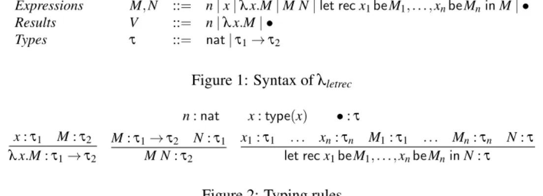
Structural rules: ` Θ,P ⇑ Γ` Θ ⇑ Γ,P Store ` Θ ⇑ N ` Θ ⇓ N Release ` P,Θ ⇓ P ` P,Θ ⇑ · Focus Negative phase: ` Θ ⇑ Γ,t− ` Θ ⇑ Γ,A ` Θ ⇑ Γ,B ` Θ ⇑ Γ,A ∧−B ` Θ ⇑ Γ ` Θ ⇑ Γ, f− ` Θ ⇑ Γ,A,B
` Θ ⇑ Γ,A ∨−B ` Θ ⇑ Γ,∀xA` Θ ⇑ Γ,A Positive phase: ` Θ ⇓ t+ ` Θ ⇓ A ` Θ ⇓ B ` Θ ⇓ A ∧+B ` Θ ⇓ Ai ` Θ ⇓ A1∨+A2 ` Θ ⇓ A[t/x] ` Θ ⇓ ∃xA Figure 2: The focused proof system LKF for classical logic.
rather limited, both in its range of “focusing behavior” and in the subsets of logic to which it could be applied. Andreoli’s result, however, applied to a full and rich logic.
Figure2presents the focused proof system for annotated propositional classical logic that is derived from the LKF proof system of Liang and Miller [11]. In that figure, P denotes a positive formula, N a negative formula, andΘ consists of positive formulas. The sequents in this proof system are of the form ` Θ ⇑ Γ and ` Θ ⇓ B where Θ is a multiset of formulas, Γ is a list of formulas, and B is a formula. The inference rules used in the negative phase are invertible while those in the positive phase are not necessarily invertible. The structural rules contain two rules that allow switching between the two kinds of sequents. Notice also that the Focus rule incorporates the contraction rule.
Theorem 1. LKF is sound and complete for classical logic. More precisely, let B be a first order formula and let ˆB be a polarization of B. Then B is provable in classical logic if and only if there is an LKF proof of ` · ⇑ ˆB [11].
Notice that polarization does not affect provability but it does affect the shape of possible LKF proofs. Focused proof systems such as LKF allow us to change the size of inference rules with which we work. Let us call individual introduction rules (such as in Figures1 and 2) “micro-rules.” An entire phase within a focused proof (the collecting together of only ⇑ sequents or only ⇓ sequent) can be seen as a “macro-rule.” In particular, consider the following derivation
` Θ,D ⇑ N1 ··· ` Θ,D ⇑ Nn ··· only ⇓ sequents here ···
` Θ,D ⇓ D ` Θ,D ⇑ ·
Here, the selection of the formula D for the focus can be taken as selecting among several macro-rules: this derivation illustrates one such macro-rule: the inference rule with conclusion ` Θ,D ⇑ · and with n ≥ 0 premises ` Θ,D ⇑ N1, . . . ,` Θ,D ⇑ Nn (where N1, . . . ,Nn are negative formulas). We shall say that this macro-rule is positive. Similarly, there is a corresponding negative macro-rule with conclusion, say, ` Θ,D ⇑ Ni, and with m ≥ 0 premises of the form ` Θ,D,C ⇑ ·, where C is a multiset of positive formulas or negative literals. In this way, focused proofs allow us to view the construction of proofs from conclusions of the form ` Θ ⇑ · by first attaching a positive macro rule (by focusing on some formula in Θ) and then attaching negative inference rules to the resulting premises until one arrives again to sequents of the form ` Θ0 ⇑ ·. Such a combination of a positive macro rule below negative macro rules is often called a bipole [2].
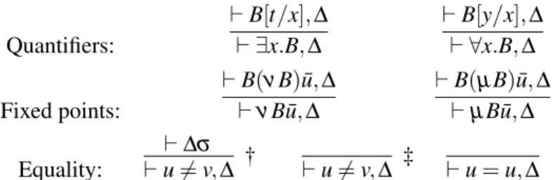
Fixed points and proof theory: An extended abstract Miller Quantifiers: ` B[t/x],∆` ∃x.B,∆ ` B[y/x],∆ ` ∀x.B,∆ Fixed points: ` B(νB) ¯u,∆ ` νB ¯u,∆ ` B(µB) ¯u,∆ ` µB ¯u,∆ Equality: ` u 6= v,∆` ∆σ † ` u 6= v,∆ ‡ ` u = u,∆
The † proviso requires the terms u and v to be unifiable andσ to be their most general unifier. The ‡ proviso requires that the terms s and t are not unifiable. The usual eigenvariable condition holds for y in the ∀ introduction rule.
Figure 3: Introduction rules for = andµ.
3 Fixed points and first-order structure
To classical logic we shall now add the two fixed point constructors µ and ν, the two first-order quan-tifiers ∀ and ∃, and the two comparison relations on first-order terms = and 6=. Notice that each pair of these connectives forms a de Morgan dual. The connectivesµ and ν are really a collection {µn}n≥0and {νn}n≥0such that the simple type ofµnand ofνnisτn→ τn, whereτnis i → ... → i → o (n occurrences of the type i). We shall not write the subscripted arity. Notice that all six of these constants are logical connectives in the sense that they all have introduction rules: furthermore, the identity rules (cut and ini-tial) are admissible. The (unfocused) proof rules for these additional connectives are given in Figure3. The rules for equality and its negation are due to Schroeder-Heister [20] and Girard [10].
Example 2. Identify the natural numbers as terms involving 0 for zero and s for successor. The following simple logic program defines two predicates on natural numbers.
nat 0 ⊂ true. nat (s X) ⊂ nat X.
leq 0 Y ⊂ true. leq (s X) (s Y ) ⊂ leq X Y. The predicate nat can be written as the fixed point
µ(λ pλx.(x = 0) ∨+
∃y.(s y) = x ∧+p y) and binary predicate leq (less-than-or-equal) can be written as the fixed point
µ(λqλxλy.(x = 0) ∨+∃u∃v.(s u) = x ∧+(s v) = y ∧+q u v).
In a similar fashion, any Horn clause specification can be made into fixed point specifications (mu-tual recursions requires standard encoding techniques). Notice the use of positively annotated logical connectives here.
Following the usual convention of classifying invertible introduction as negative connectives, ∀ and 6= are negative and their duals ∃ and = are positive. Since the two fixed points are (currently) indistin-guishable (they have the same introduction rules), we arbitrarily classifyµ as positive and ν as negative. The focused versions of the introduction rules for these connectives is given in Figure4. Notice now that focusing phases can involve long chains of unfoldings. For example, the fixed points in Example2are encoded using entirely positive connectives. Thus, if the focused sequent ` Θ ⇓ leq m n has a proof, it has a proof that involves exactly one macro-rule. As the following example illustrates, it is now possible to put an arbitrary (Horn clause) computation within a (macro) rule.
` Θ ⇓ B[t/x] ` Θ ⇓ ∃x.B ` Θ ⇑ Γ,B[y/x] ` Θ ⇑ Γ,∀x.B ` Θ ⇓ u = u ` Θσ ⇑ Γσ ` Θ ⇑ Γ,u 6= v † ` Θ ⇑ Γ,u 6= v ‡ ` Θ ⇑ Γ,B(νB) ¯u ` Θ ⇑ Γ,νB ¯u ` Θ ⇓ B(µB) ¯u ` Θ ⇓ µB ¯u
Figure 4: Focused inference rules for = andµ. The proviso † and ‡ and the definition of σ are the same as above.
Example 3. Consider proving the positive focused sequent
` Θ ⇓ (leq m n ∧+N1)∨+(leq n m ∧+N2),
where m and n are natural numbers and leq is the fixed point expression displayed above. If both N1and N2are negative formulas, then there are exactly two possible macro rules with this conclusion: one with premise ` Θ ⇑ N1when m ≤ n and one with premise ` Θ ⇑ N2when n ≤ m (thus, if m = n, either premise is possible). In this sense, a macro inference rule can contain an entire Prolog-style computation.
The following example illustrates that fixed points can be used to describe a typical query from model checking.
Example 4. Assume that first-order terms encode process and action expressions such as are found in CCS. The usual notion of one-step transition can generally be written using a simple, recursive Horn clause program: hence, the ternary relation P−→ PA 0 can be encoded using a purely positive formula. The notion of simulation is then the (greatest) fixed point of the equivalence
sim P Q ≡ ∀P0∀A[P−→ PA 0⊃ ∃Q0[Q−→ QA 0∧ sim P0Q0]]. We can then chose to write the sim relation as the expression
νλsλPλQ.∀P0∀A[P−→ PA 0⊃ ∃Q0[Q−→ QA 0∧ s P0Q0]]
(Here, we are assuming that the implication B ⊃ C is rendered as B⊥∨−C in the polarized setting.) Although the body of this definition looks complex, it is, in fact, composed of exactly two “macro con-nectives” (a bipole). The expression ∀P0∀A[P−→ PA 0⊃ ·] is a purely negative formula and its “intro-duction” is invertible: since all possible actions A and continuations P0must be computed, there are no choices to be made in building a proof for this expression. On the other hand, focusing on the expression ∃Q0[Q−→ QA 0∧+·] yields a non-invertible, positive macro rule. In this way, the focused proof system is aligned directly with the structure of the actual (model-checking) problem.
The fact that an entire computation can fit within a macro rule (using purely positive fixed point expressions) provides a great deal of flexibility in designing inference rules. Such flexibility allows inference rules to be designed so that they correspond to an “action” within a given computational system. If one takes seriously using only macro rules (and hiding the details of the micro rules) then placing arbitrary computation within a macro inference rule is probably too much: the term “inference rule” is usually reserved for decidable steps. Thus, some care should be exercised in balancing the complexity of a macro rule with the needs of proof systems to have their correctness be decidable.
Fixed points and proof theory: An extended abstract Miller
` Γ,B(µB) ¯u ` Γ, µB ¯u µ
` Γ,S ¯u ` BSx,(Sx)⊥
` Γ,νB ¯u ν ` µB ¯u,ν ¯B ¯u µν
The variable S denotes a closed term of typeτn, where the arity ofν is n. Also, x is an eigenvariable of the proof.
Figure 5: Inference rules for induction and co-induction.
Large macro rules can easily be broken up, if desired, by the use of delays. Within LKF, we can define the delaying operators
∂+(B) = B ∧+t+ and ∂−(B) = B ∧−t−.
Clearly, B, ∂−(B), and∂+(B) are all logically equivalent but ∂−(B) is always negative and∂+(B) is always positive. If one wishes to break a positive macro rule resulting from focusing on a given positive formula into smaller pieces, then one can insert∂−(·) into that formula. Similarly, inserting ∂+(·) can limit the size of a negative macro rule. By inserting many delay operators, a focused proof can be made to emulate an unfocused proof [11].
4 Induction and co-induction rules
Treating fixed points simply by unfolding is, of course, limited. For example, while it is easy to define fixed points that describe the notions of “natural number”, “even”, and “odd”, it is not possible to prove that every natural number is either even or odd. While one can simply write the appropriate formula stating that theorem, attempts at proofs of it will lead only to potentially infinite unfoldings. What is missing, of course, is induction. To this end, consider the three inference rules displayed in Figure5 (taken from [3,6]). Notice that theµν rule is the only form of the initial rule that we shall need in this proof system. Here, the negation B of a body B is defined asλ p.λ~x.(B(λ~x.(p~x)⊥)~x)⊥. A body B is said to be monotonic when for any variables p and ¯t, the negation normal andλ-normal form of Bp¯t does not contain any negated instance of p. We shall assume that all bodies are monotonic.
Notice that the rule called ν is the rule for co-induction. If we write sequents as two sided, then moving this rule to the left-side as an introduction rule for µ yields the usual induction rule. Thus, induction and co-induction are treated as perfect duals of each other.
Proposition 5. The following inference rules are derivable:
` P,P⊥ init ` Γ
,B(νB) ¯u ` Γ,νB ¯u νR
These results are standard, cf. [21]. The proof of the second one relies on monotonicity and is obtained by applying theν rule with B(νB) as the co-invariant. As a result of this proposition, we can replace the inference rules forµ and ν given in Figure3with the rules in Figure5. It is also the case that µ and ν are now canonical. Such canonicity is gained, however, by the rather “high-price” of using an inference rule (theν rule) that involves a higher-order variable (the invariant).
Baelde [3,4] has proved the (relative) completeness of the focused inference rules in Figure6in the context of MALL: his proof involves some rather complex arguments for treating the higher-order nature of the induction/co-induction rule. That proof should, however, lift to the setting described here where classical logic replaces MALL.
Notice that in the ⇑ phase, one chooses between doing (co)induction on νB¯t and freezing the fixed point expression by moving it to the left of the ⇑. Since such a ν-expression is assigned a negative
` Γ ⇑ S¯t,∆ `⇑ BS~x,S~x⊥ ` Γ ⇑ νB¯t,∆ ~x new ` Γ,νB¯t ⇑ ∆ ` Γ ⇑ νB¯t,∆ ` Γ ⇓ B(µB)~x ` Γ ⇓ µB~x ` νB~x ⇓ µB~x
Figure 6: Focused proof rules for the fixed point connectives
polarity, the Focus rule can never move it from the left of the arrow to the right. Thus, aν-expression on the left of the ⇑ arrow can only be used to match its dual of the right ⇓ in the (focused version of the) µν rule. For more about these rules for (co)induction, see the Baelde’s PhD thesis [3] or the theorem prover based on that work [7].
5 The unity of computational logic
The proof theory of fixed points offers us a framework for comparing and combining computation, model checking, and theorem proving. The differences between these three activities can be characterized by their different uses of fixed points. Logic programming involves may behavior only, which involves unfolding fixed points and non-deterministically picking a path to a success. On the other hand, both model checking and theorem proving deal with must as well as may behavior. These two differ in that model checkers generally assume finite fixed points (or have specialized methods for handling loops) while (inductive) theorem provers use invariants to characterize possible infinite unfoldings. Given these rough descriptions, it is possible to see rich ways that these activities can fit together into one system (and one logic!) and enhance each other: for example, a theorem prover might prove certain symmetry lemmas (via induction) and these could be used in the model checker to reduce search space. Similarly, tabling within model checkers can be seen as lemma generation in theorem provers [16]. Also, as we have seen, logic programming-style computation can be inserted within the inference rules used in both model checking and theorem proving.
6 Related work
The proof theory of fixed points described here is largely taken from the recent papers of Baelde [3,7]. While Baelde largely considered adding fixed point to MALL, he has also shown how that combination directly treats important subsets of intuitionistic logic. Miller and Saurin [17] have also considered fixed points using dialog games which are known to be closely related to focused proof systems. This work builds on earlier work by McDowell, Miller, and Tiu [13,21]. The work on cyclic proofs by, say, Santocanale [19] and Brotherston and Simpson [8], is a related but alternative approach to the treatment of induction within proofs.
Acknowledgments: I wish to thank David Baelde and the anonymous reviewers of this abstract for their comments.
References
[1] Jean-Marc Andreoli. Logic programming with focusing proofs in linear logic. J. of Logic and Computation, 2(3):297–347, 1992.
[2] Jean-Marc Andreoli. Focussing and proof construction. Annals of Pure and Applied Logic, 107(1):131–163, 2001.
Fixed points and proof theory: An extended abstract Miller
[3] David Baelde. A linear approach to the proof-theory of least and greatest fixed points. PhD thesis, Ecole Polytechnique, December 2008.
[4] David Baelde. Least and greatest fixed points in linear logic. Submitted, October 2009.
[5] David Baelde, Andrew Gacek, Dale Miller, Gopalan Nadathur, and Alwen Tiu. The Bedwyr system for model checking over syntactic expressions. In Frank Pfenning, editor, 21th Conference on Automated Deduction (CADE), number 4603 in LNAI, pages 391–397. Springer, 2007.
[6] David Baelde and Dale Miller. Least and greatest fixed points in linear logic. In N. Dershowitz and A. Voronkov, editors, International Conference on Logic for Programming and Automated Reasoning (LPAR), volume 4790 of LNCS, pages 92–106, 2007.
[7] David Baelde, Dale Miller, and Zachary Snow. Focused inductive theorem proving. Accepted to IJCAR 2010., 2010.
[8] James Brotherston and Alex Simpson. Complete sequent calculi for induction and infinite descent. In 22th Symp. on Logic in Computer Science, pages 51–62, 2007.
[9] Roy Dyckhoff. Contraction-free sequent calculi for intuitionistic logic. J. of Symbolic Logic, 57(3):795–807, September 1992.
[10] Jean-Yves Girard. A fixpoint theorem in linear logic. A posting to [email protected], February 1992. [11] Chuck Liang and Dale Miller. Focusing and polarization in linear, intuitionistic, and classical logics.
Theo-retical Computer Science, 410(46):4747–4768, 2009.
[12] P. Lincoln, J. Mitchell, A. Scedrov, and N. Shankar. Decision problems for propositional linear logic. Annals Pure Applied Logic, 56:239–311, 1992.
[13] Raymond McDowell and Dale Miller. Reasoning with higher-order abstract syntax in a logical framework. ACM Trans. on Computational Logic, 3(1):80–136, 2002.
[14] Dale Miller. Finding unity in computational logic. In ACM-BCS-Visions Conference, April 2010.
[15] Dale Miller, Gopalan Nadathur, Frank Pfenning, and Andre Scedrov. Uniform proofs as a foundation for logic programming. Annals of Pure and Applied Logic, 51:125–157, 1991.
[16] Dale Miller and Vivek Nigam. Incorporating tables into proofs. In J. Duparc and T. A. Henzinger, editors, CSL 2007: Computer Science Logic, volume 4646 of LNCS, pages 466–480. Springer, 2007.
[17] Dale Miller and Alexis Saurin. A game semantics for proof search: Preliminary results. In Proceedings of the Mathematical Foundations of Programming Semantics (MFPS05), number 155 in Electronic Notes in Theoretical Computer Science, pages 543–563, 2006.
[18] Vivek Nigam and Dale Miller. Algorithmic specifications in linear logic with subexponentials. In ACM SIGPLAN Conference on Principles and Practice of Declarative Programming (PPDP), pages 129–140, 2009.
[19] Luigi Santocanale. A calculus of circular proofs and its categorical semantics. In Proceedings of Foundations of Software Science and Computation Structures (FOSSACS02), number 2303 in LNCS, pages 357–371. Springer-Verlag, January 2002.
[20] Peter Schroeder-Heister. Rules of definitional reflection. In M. Vardi, editor, Eighth Annual Symposium on Logic in Computer Science, pages 222–232. IEEE Computer Society Press, IEEE, June 1993.
[21] Alwen Tiu. A Logical Framework for Reasoning about Logical Specifications. PhD thesis, Pennsylvania State University, May 2004.
Department of Informatics & Telecommunications, University of Athens, Greece [email protected]
We examine two successful application domains for fixed-point theory, namely (non-monotonic) logic programming and Boolean grammars. We demonstrate that these two areas are quite close, and as a result interesting ideas from one area appear to have interesting counterparts in the other one.
Negation in Logic Programming: We present a recent [RW05] purely model-theoretic characterization of the semantics of logic programs with negation. The new semantics provides a logical basis for the classical well-founded semantics of logic programs [vGRS91]. The proposed approach uses a truth domain that has an uncountable linearly ordered set of truth values between False (the minimum element) and True (the maximum), with a Zero element in the middle. Under the new semantics, every logic program with negation has a unique minimum model which can be constructed as the least fixed point of the immediate consequence operator of the program. The main benefits of the new construction is that it provides a purely logical characterization of negation-as-failure and a better understanding of the fixed-point semantics of non-monotonic logic programming.
Boolean Grammars: These new grammars [Okh04] extend the context-free ones by allowing conjunction and negation in the right hand sides of rules. It has been demonstrated that Boolean grammars can be parsed efficiently and that they can express interesting languages that are not context-free. Despite their simplicity, Boolean grammars proved to be non-trivial from a semantic point of view. In particular, the use of negation makes it difficult to define a simple derivation-style semantics (such as the familiar one for context-free languages). We present the well-founded construction for Boolean grammars [KNR09], which provides the first general solution to the problem of assigning a proper meaning to every Boolean grammar. Our results indicate that many-valued formal language theory is the appropriate mathematical machinery underlying Boolean grammars.
References
[KNR09] Kountouriotis, V., Nomikos, Ch., Rondogiannis, P.: Well-Founded Semantics for Boolean Grammars.
Information and Computation.207(9) (2009) 945–967.
[Okh04] Okhotin, A.: Boolean Grammars. Information and Computation.194(1) (2004) 19–48.
[RW05] Rondogiannis, P., Wadge, W., W.: Minimum Model Semantics for Logic Programs with
Negation-as-Failure. ACM Transactions on Computational Logic.6(2) (2005) 441–467.
[vGRS91] van Gelder, A, Ross, K., A., Schlipf, J., S.: The Well-Founded Semantics for General Logic Programs.
Journal of the ACM.38(3) (1991) 620–650.
IT University of Copenhagen [email protected] Saarland University [email protected] IT University of Copenhagen [email protected] Abstract
We give a model for Nakano’s typed lambda calculus with guarded recursive definitions in a category of metric spaces. By proving a computational adequacy result that relates the interpretation with the operational semantics, we show that the model can be used to reason about contextual equivalence.
1 Introduction
Recent work in semantics of programming languages and program logics has suggested that there might be a connection between metric spaces and Nakano’s typed lambda calculus with guarded recursive definitions [8]. In this paper we show that is indeed the case by developing a model of Nakano’s calculus in a category of metric spaces and by showing that the model is computationally adequate. The latter is done with the use of a logical relation, whose existence is non-trivial because of the presence of recursive types. We define the relation in a novel indexed way, inspired by step-indexed models for operational semantics [2].
For space reasons, we can only briefly hint at some of the motivating applications in semantics: In [4], Birkedal et al. gave a model of a programming language with recursive types, impredicative polymorphism and general ML-style references. The model is a Kripke model, where the set of worlds is a recursively defined metric space (with the recursion variable in negative position). A simplified variant of the recursive equation can be formulated in a version of Nakano’s calculus.
Pottier [9] has recently suggested to use Nakano’s calculus as a calculus of kinds in an extension of Fω with recursive kinds, which can serve as a target calculus for a store-passing translation of a language with ML-style references. The model we present here can be extended to a model of Fω with recursive kinds by indexing complete uniform per’s over metric spaces.
Hinze [6] has shown, in the context of Haskell streams, how the uniqueness of fixed points of con-tractive functions in an operational setting can be used for verification. Nakano’s calculus can be used to formalize such arguments, and in our model unique fixed points for contractive functions do exist.
For reasoning about imperative interactive programs, Krishnaswami et al. [7] related an efficient imperative implementation to a simple model of functional reactive programming. In current unpublished work by Krishnaswami on extending this to higher-order programs, metric spaces are being used to model the functional reactive programs to capture that all uses of recursion are guarded. A logical relation is used to relate the functional reactive programs and the imperative implementation thereof; that logical relation is defined using ideas that seem similar to those we are using in our logical relation for the adequacy proof in Section3.
In the remainder of the paper, we present (our version of) Nakano’s calculus (Section2), define the denotational semantics and prove that it is computationally adequate (Section3), briefly discuss some closely related work (Section4), and conclude with some comments about future work.
A Metric Model of Lambda Calculus with Guarded Recursion Birkedal et al. Γ,x:τ ` x : τ Γ ` n : Int Γ,x:τ ` t : σ Γ ` λx:τ.t : τ → σ Γ ` t1: •n(τ → σ) Γ ` t2: •nτ Γ ` t1t2: •nσ Γ ` t1:τ1 Γ ` t2:τ2 Γ ` (t1,t2):τ1× τ2 Γ ` t : •n(τ 1× τ2) Γ ` proji(t) : •nτi •Γ ` t : •τ Γ ` t : τ Γ ` t : •τi, j Γ ` Ini, j(t) : tyi Γ ` t : tyi Γ,x1:•τi,1` t1:τ . . . Γ,xik:•τi,ki` tki:τ
Γ ` case t of Ini,1(x1)⇒ t1|...| Ini,ki(xki)⇒ tki :τ
Γ ` t : τ ` τ ≤ σ
Γ ` t : σ
Figure 1: Typing rules of Nakano’s lambda calculus
` τ ≤ σ ` •τ ≤ •σ ` τ0≤ τ ` σ ≤ σ0 ` τ → σ ≤ τ0→ σ0 ` τ ≤ τ0 ` σ ≤ σ0 ` τ × σ ≤ τ0× σ0 ` τ ≤ •τ ` τ → σ ≤ •τ → •σ ` •τ → •σ ≤ •(τ → σ) ` τ × σ ≤ •τ × •σ ` •τ × •σ ≤ •(τ × σ) Figure 2: Subtyping
2 Nakano’s Lambda Calculus
In this section we recall the typed lambda calculus of Nakano [8]. It allows certain forms of guarded recursive definitions, and tracks guardedness via a modality in the type system. We shall show that this modality can be understood semantically as a scaling operation of the distances in a metric space.
The precise language considered below differs from that presented by Nakano in [8] in that we assume a fixed number of “global” (possibly mutually recursive) datatype declarations. In contrast, Nakano includes equi-recursive types of the form µX.A (subject to some well-formedness conditions that ensure formal contractiveness, and a type equivalence relation).
Syntax and typing. We assume that there is a fixed number of type identifiers ty1, . . . ,tyn, each as-sociated with a recursive data type equation in the style of Haskell or ML that specifies constructors Ini,1, . . . ,Ini,ki:
data tyi=Ini,1ofτi,1|...| Ini,ki ofτi,ki . (1) The typesτi,1, . . . ,τi,ki that appear on the right hand side of (1) are built up from ground types b (for sim-plicity, we restrict ourselves to Int) and the identifiers ty1, . . . ,tyn, using product and function space and the unary type constructor ‘•’ (referred to as ‘later’ modality in recent work on step-indexed semantics [3]). One concrete instance of (1) is a type of infinite sequences ofτ’s: data seqτ =Cons ofτ × seqτ. In general, these declarations need not be monotone, however, and the identifiers tyimay also appear in negative positions. For instance, Nakano [8, Ex. 1] considers the type data u = Fold of u → τ. With this type, the fixed point combinator Y from untyped lambda calculus has type (•τ → τ) → τ; thus, it is not necessary to include a primitive for recursion.
Terms and their types are given in Figure1. The type system uses the subtyping relation defined in Figure2(omitting the reflexivity and transitivity rules). Intuitively, the type •τ may be understood as the set of values of typeτ that need to be guarded by a constructor. This intuition explains the two rules
for typing constructor applications and pattern matching in Figure1: The application of a constructor lets one remove the outermost modal operator, and it also folds the recursive type. Conversely, the case construct removes a constructor, and the typing rule records this fact by applying the modality to the type of the bound variables. The typing rules for function application and component projections are also generalized to take care of the modal operator. We write Tm(τ) for the set of closed terms of type τ.
Operational semantics and contextual equivalence. The operational semantics consists of the usual (deterministic, call-by-name) reduction rules of lambda calculus with constructor types. One does not reduce under constructors: every term of the form Ini, j(t) is a value. We take contextual equivalence as our notion of program equivalence. Formally, we observe the values that terms yield when plugged into closing, base-type valued contexts: Let us write ` C : (Γ0.τ0)( (Γ . τ) for a context C if Γ ` C[t] : τ wheneverΓ0` t : τ0. Then t1and t2are contextually equivalent, writtenΓ ` t1' t2:τ, if Γ ` t1:τ and Γ ` t2:τ, and for all ` C : (Γ.τ) ( (/0.Int) and n ∈ N, C[t1]→ n ⇔ C[t∗ 2]→ n.∗
3 Denotational Semantics
We give a denotational semantics of types and terms in the category of complete, 1-bounded ultrametric spaces and non-expansive maps between them.
Ultrametric spaces. We briefly recall some basic definitions and results about metric spaces [10]. A 1-bounded ultrametric space (X,d) is a metric space where the distance function d : X × X → R takes values in the closed interval [0,1] and satisfies the “strong” triangle inequality d(x,y) ≤ max{d(x,z),d(z,y)}. A metric space is complete if every Cauchy sequence has a limit. Because of the use of max in the above inequality, rather than ‘+’ as for the weaker triangle inequality of metric spaces in general, a sequence (xn)n∈N in an ultrametric space (X,d) is a Cauchy sequence if for every ε > 0 there exists n ∈ N such that d(xk,xk+1)≤ ε for every k ≥ n.
A function f : X1→ X2between metric spaces (X1,d1), (X2,d2)is non-expansive if d2(f (x), f (y)) ≤ d1(x,y) for all x,y ∈ X1. It is contractive if there exists someδ < 1 such that d2(f (x), f (y)) ≤ δ ·d1(x,y) for all x,y ∈ X1. The complete, 1-bounded, non-empty, ultrametric spaces and non-expansive functions between them form a Cartesian closed category CBUltne. Products are given by the set-theoretic product where the distance is the maximum of the componentwise distances. The exponential (X1,d1)→ (X2,d2) has the set of non-expansive functions from (X1,d1)to (X2,d2)as underlying set, and the distance func-tion is given by dX1→X2(f ,g) = sup{d2(f (x),g(x)) | x ∈ X1}.
A functor F : (CBUltopne)n× CBUltnne−→ CBUltne is locally non-expansive if d(F( f ,g),F( f0,g0))≤ max{d( f1,f10),d(g1,g01), . . . ,d( fn,fn0),d(gn,g0n)} for all non-expansive f = ( f1, . . . ,fn), f0= (f10, . . . ,fn0), g = (g1, . . . ,gn) and g0 = (g01, . . .g0n). It is locally contractive if there exists some δ < 1 such that d(F( f ,g),F( f0,g0))≤ δ · max{d( f1,f0
1),d(g1,g01), . . . ,d( fn,fn0),d(gn,g0n)}. Note that the factor δ is the same for all hom-sets. By multiplication of the distances of (X,d) with a non-negative shrinking factor δ < 1, one obtains a new ultrametric space, δ ·(X,d) = (X,d0)where d0(x,y) =δ ·d(x,y). By shrinking, a locally non-expansive functor F yields a locally contractive functor (δ ·F)(X,Y) = δ ·(F(X,Y)).
It is well-known that one can solve recursive domain equations in CBUltne by an adaptation of the inverse-limit method from classical domain theory:
Theorem 1 (America-Rutten [1]). Let Fi: (CBUltopne)n× CBUltnne−→ CBUltne be locally contractive functors for i = 1,...,n. Then there exists a unique (up to isomorphism) X = (Xk,dk)k∈ CBUltnne such that (Xi,di) ∼= Fi(X,X) for all i.
A Metric Model of Lambda Calculus with Guarded Recursion Birkedal et al.
The metric spaces we consider below are bisected, meaning that all non-zero distances are of the form 2−nfor some natural number n ≥ 0. When working with bisected metric spaces, the notation x=n y means that d(x,y) ≤ 2−n. Each relation=n is an equivalence relation because of the ultrametric inequality; we are therefore justified in referring to the relation=n as “n-equality.” Since the distance of a bisected metric space is bounded by 1, the relation x=0 y always holds. Moreover, the n-equalities become finer as n increases, and x = y if x=n y holds for all n. Finally, a function f : X1→ X2between bisected metric spaces is non-expansive iff x1=xn 01⇒ f (x1)=n f (x01), and contractive iff x1=xn 01⇒ f (x1)n+1= f (x01)for all n. Denotational semantics of Nakano’s lambda calculus. We can now define the interpretation of types and terms in CBUltne. More precisely, by induction on the type τ we define locally non-expansive functors Fτ : (CBUltopne)n× CBUltnne−→ CBUltne, by separating positive and negative occurrences of the identifiers ty1, . . . ,tyninτ:
FInt(X,Y ) = (Z,d), where d is the discrete metric Ftyi(X,Y ) = Yi
Fτ1×τ2(X,Y ) = Fτ1(X,Y ) × Fτ2(X,Y ) Fτ1→τ2(X,Y ) = Fτ1(Y,X) → Fτ2(X,Y )
F•τ(X,Y ) =12· Fτ(X,Y )
Now consider the functors Fi: (CBUltopne)n× CBUltnne−→ CBUltnefor i = 1,...,n, defined by
Fi(X,Y ) =12· Fτi,1(X,Y ) + ... +12· Fτi,ki(X,Y ) . (2) Because of the shrinking factor 1/2 in (2), each Fi is in fact locally contractive. Theorem 1therefore gives a unique fixed point D withιi: Fi(D,D) ∼= Difor all i. We use D to give the semantics of types:
JτK=defFτ(D,D) .
Example 2 (Interpretation of streams). On streams, the semantics yields the “natural” metric. In fact, since JseqτK ∼=12· (JτK × JseqτK) we have
dJseqτK(s1s2. . . ,s10s02. . . )≤ 2−n ⇔ dJτK(s1,s01)≤ 2−(n−1) ∧ dJseqτK(s2s3. . . ,s02s03. . . )≤ 2−(n−1). In particular, because of the discrete metric on JIntK, for seqInt this means s =n s0 holds if s1 = s0
1, . . . ,sn−1=s0n−1, i.e., if the common prefix of s and s0 has at least length n − 1, and s = s0if si=s0ifor all i ∈ N.
For each subtyping derivation∆ of a judgement ` τ ≤ σ we define a corresponding coercion function, i.e., a non-expansive function J∆K : JτK → JσK. First note that, for each of the 5 subtyping axioms ` τ ≤ σ in Figure2(as well as the reflexivity axiom), the underlying sets of JτK and JσK are equal. Thus we can define J∆K as the identity on the underlying sets, and it is easy to check that ∆ is in fact non-expansive.1
If ∆ is obtained from ∆1 and ∆2 by an application of the transitivity rule, then J∆K is defined as the composition of J∆1K and J∆2K. Finally, for each of the 3 structural rules in Figure2, we use the functorial property of the respective type constructor to define J∆K from the coercions of the subderivations. It follows by induction that the coercion determined from any derivation∆ of ` τ ≤ σ is the identity on the underlying set of JτK, and hence independent of ∆.
1Note however that even though the underlying sets are the same, the inclusion of J•(τ → σ)K into J•τ → •σK fails to be
Each term x1:τ1, . . . ,xn:τn` t : τ denotes a non-expansive function JtK : Jτ1K × ... × JτnK → JτK
which is defined by induction on the typing derivation. The cases of lambda abstraction, application, pairing and projections are given in terms of the cartesian closed structure on CBUltne. From the def-inition of the type interpretation it follows thatιi is an isomorphism between 12· Jτi,1K + ... +12· Jτi,kiK and JtyiK. Together with the injections from J•τi, jK = 12· Jτi, jK into the sum, this isomorphism is used to interpret the constructors and pattern matching of the calculus:
JIni, j(t)K(~a) = (ιi◦inj◦JtK)(~a) and Jcase t of Ini,1(x1)⇒ t1|...| Ini,ki(xki)⇒ tkiK(~a) = JtjK(~a,a) whereι−1
i (JtK(~a)) = inj(a) for some 1 ≤ j ≤ kiand a ∈ Jτi, jK. We obtain a model that is sound: Theorem 3 (Soundness). If /0 ` t : τ and t1→ t2then Jt1K = Jt2K in JτK.
Remark 4 (Recursive definitions). In [8] Nakano shows that the fixed point combinator Y from untyped lambda calculus can be represented byλ f .∆f(Fold(∆f))where∆f =λx. f (case x of Fold(y) ⇒ yx) and the data type data u = Fold of u → τ is assumed, and that this term has type (•τ → τ) → τ. Note that in the above interpretation, where the modality is interpreted by scaling the distances by 1/2, the type •τ → τ denotes the set of all non-expansive functions 12· JτK → JτK, or equivalently (by the bisectedness of JτK) the contractive functions on JτK. Such functions have a unique fixed point in JτK by the Banach fixed point theorem, and we can show that Y indeed returns this fixed point since f (JYK f ) = JYK f .
As an alternative to this coding, we could introduce a recursion operator rec : (•τ → τ) → τ for each τ as a primitive, with reduction rule rec t → t (rec t), and use the above observation for its interpretation. Computational adequacy. We now relate the interpretation of lambda terms in the metric model and their operational behaviour. In particular, we prove that the semantics is sound for reasoning about contextual equivalence: if two terms have the same denotation then they are contextually equivalent.
The general idea of the adequacy proof is standard: the universal quantification over contexts prevents a direct inductive proof, so we use the compositionality of the denotational semantics and construct a (Kripke) logical relation between semantics and syntax. More precisely, we consider the family (Rk
τ)kτ of relations indexed by typesτ and natural numbers k, where Rk
τ ⊆ JτK × Tm(τ) is given by: n RkIntt ⇔ t→ n∗ (a1,a2)Rkτ1×τ2t ⇔ a1Rkτ1 proj1(t) ∧ a2Rkτ2 proj2(t) f Rkτ1→τ2t ⇔ ∀ j,a1,t1. j ≤ k ∧ a1Rτj1t1 ⇒ f a1R j τ2t t1 a Rk•τt ⇔ k > 0 ⇒ a Rk−1τ t a Rk
tyit ⇔ ∃a0,t0.a = (ιi◦inj)(a0) ∧ t→ In∗ i, j(t0) ∧ a0Rk•τi, jt0 Note that it is the natural number index which lets us define the relations Rk
τ inductively in the presence of recursive types tyi. We prove the ‘fundamental property’ by induction on typing derivations:
Proposition 5. If Γ ` t : τ, k ∈ N, and aiRkτi tifor all xi:τiinΓ, then JtK(~a) R k
τt[~x:=~t].
Proof sketch. By induction on the derivation ofΓ ` t : τ. The proof uses the closure of the relations under the operational semantics, the downwards closure (Kripke monotonicity) in k, and the closure under the coercions determined by the subtyping relation.
A Metric Model of Lambda Calculus with Guarded Recursion Birkedal et al.
Now adequacy is easily proved. In fact, given Γ ` t1:τ, Γ ` t2:τ and ` C : (Γ . τ) ( (/0 . Int), and C[t1]→ n for some n ∈ N, then JC[t∗ 2]K = JC[t1]K = n follows from the assumption Jt1K = Jt2K and Theorem3. By Proposition5, JC[t2]K RIntk C[t2], and therefore n RkIntC[t2]holds. But by definition this means C[t2]→ n, and with a symmetric argument the claim∗ Jt1K = Jt2K ⇒ Γ ` t1' t2:τ follows.
Apart from using the semantics directly to reason about contextual equivalence, we can also use com-putational adequacy to derive more abstract proof principles from it. For instance, by the characterization of the metric on seqIntgiven in Example2and the fact that there are closed terms getn: seqInt→ •nInt that yield the n-th element of a sequence, we obtain a variant of Bird and Wadler’s take lemma: if getnt1 and getnt2 reduce to the same value, for each n ∈ N, then /0 ` t1' t2: seqInt. Similarly, we can exploit the uniqueness of fixed points of contractive equations also in the operational setting: if there exists a closed term f : •τ → τ such that f t1 and t1 are convertible, and also f t2 and t2 are convertible, then /0 ` t1' t2:τ. See, for instance, Hinze’s article [6] for numerous applications of such a unique fixed point principle phrased in the context of Haskell streams, and Pottier’s work [9] for a similar application to establish type equivalences in the context of Fω with recursive kinds.
4 Related Work
Metric semantics of PCF. Escard´o [5] presents a metric model of PCF. One can, almost,2 factor his
interpretation of PCF into two parts: (1) a syntactic translation from PCF to Nakano’s calculus, extended with constants for integer operations and a booleans, and (2) the metric interpretation of Nakano’s calcu-lus presented here. The basic idea of the syntactic translation is that a potentially divergent PCF term of integer type is translated into a term of the recursive type Ints=Done of Int | Next of Ints. After evaluat-ing such a term, one either obtains an actual integer answer, Done(n), or a new term that one can evaluate in the hope of eventually getting an integer answer. PCF function types are translated to function types.
Now, for all typesτ that are used to interpret PCF types, one defines a term delay : •τ → τ; this term is used to define the fixed-point combinator of PCF in terms of the fixed-point combinator of our calculus (Remark4). See Escard´o for more details. Intuitively, the idea is that unfolding a recursive definition takes a “computation step,” which will be visible as an extra Next in the final answer of type Ints. Escard´o shows an adequacy result which implies that the semantics of a PCF term does indeed match the number of unfoldings of the fixed-point combinator; the same information can be obtained from our adequacy proof using the definition of the logical relation on recursive types. Escard´o gives two adequacy proofs, the first of which uses a Kripke logical relation as in our adequacy proof.
Since Escard´o considers PCF, he does not treat recursively defined types, as we do here.
5 Conclusion and Future Work
We have presented a computationally adequate metric model of lambda calculus with guarded recursion. It complements Nakano’s realizability interpretations [8], and it explains the modality in terms of scaling. We conjecture that an adaptation of the present model can be used to give a model for focusing proof systems with recursive types [11].
2Due to the syntactic restrictions on recursive types in our variant of Nakano’s calculus, the metrics on PCF ground types (and
References
[1] P. America and J. J. M. M. Rutten. Solving reflexive domain equations in a category of complete metric spaces. Journal of Computer and System Sciences, 39(3):343–375, 1989.
[2] A. W. Appel and D. McAllester. An indexed model of recursive types for foundational proof-carrying code. ACM Transactions on Programming Languages and Systems, 23(5):657–683, 2001.
[3] A. W. Appel, P.-A. Melli`es, C. D. Richards, and J. Vouillon. A very modal model of a modern, major, general type system. In Proceedings of POPL, pages 109–122, 2007.
[4] L. Birkedal, K. Støvring, and J. Thamsborg. Realizability semantics of parametric polymorphism, general references, and recursive types. In Proceedings of FOSSACS, pages 456–470, 2009.
[5] M. Escard´o. A metric model of PCF. Presented at the Workshop on Realizability Semantics and Applications, June 1999. Available at the author’s web page.
[6] R. Hinze. Functional pearl: streams and unique fixed points. In Proceedings of ICFP, pages 189–200, 2008. [7] N. Krishnaswami, L. Birkedal, and J. Aldrich. Verifying event-driven programs using ramified frame
prop-erties. In Proceedings of TLDI, pages 63–76, 2010.
[8] H. Nakano. A modality for recursion. In Proceedings of LICS, pages 255–266, 2000. [9] F. Pottier. A typed store-passing translation for general references. Submitted, Apr. 2010.
[10] M. B. Smyth. Topology. In Handbook of Logic in Computer Science, volume 1. Oxford Univ. Press, 1992. [11] N. Zeilberger. The Logical Basis of Evaluation Order and Pattern-Matching. PhD thesis, Carnegie Mellon
Recursive Properties on Recursively Defined Metric Spaces
Lars Birkedal IT University of Copenhagen [email protected] Jan Schwinghammer Saarland University [email protected] Kristian Støvring IT University of Copenhagen [email protected] AbstractFrame and anti-frame rules have been proposed as proof rules for modular reasoning about pro-grams. Frame rules allow one to hide irrelevant parts of the state during verification, whereas the anti-frame rule allows one to hide local state from the context. We give a possible worlds seman-tics for Chargu´eraud and Pottier’s type and capability system including frame and anti-frame rules, based on the operational semantics and step-indexed heap relations. The worlds are constructed as a recursively defined predicate on a recursively defined metric space, which provides a considerably simpler alternative compared to a previous construction.
1 Introduction
Reasoning about higher-order stateful programs is notoriously difficult, and often involves the need to track aliasing information. A particular line of work that addresses this point are substructural type systems with regions, capabilities and singleton types [1,7,8]. In this context, Pottier [9] presented the anti-frame rule as a proof rule for hiding local state. It states that (the description of) a piece of mutable state that is local to a procedure can be removed from the procedure’s external interface (expressed in the type system). The benefits of hiding local state include simpler interface specifications, simpler reasoning about client code, and fewer restrictions on the procedure’s use because of potential aliasing. Thus, in combination with frame rules that allow the irrelevant parts of the state to be hidden during verification, the anti-frame rule provides an important ingredient for modular reasoning about programs. Soundness of the frame and anti-frame rules is subtle, and relies on properties of the programming language. Pottier [9] sketched a proof for the anti-frame rule by a progress and preservation argument, resting on assumptions about the existence of certain recursively defined types. Subsequently, Schwing-hammer et al. [12] investigated the semantic foundations of the anti-frame rule by identifying sufficient conditions for its soundness, and by instantiating their general setup to prove soundness for a separation logic variant of the rule. The latter was done by giving a Kripke model where assertions are indexed over recursively defined worlds. The recursive domain equation involved functions that should be monotonic with respect to an order relation that is specified using the isomorphism of the solution itself and an op-erator on the recursively defined worlds. This means that the standard existence theorems do not appear to apply, and thence we had to give the solution by a laborious explicit inverse-limit construction [12].
Here we explore an alternative approach, which consists of two steps. First, we consider a recursive metric space domain equation without any monotonicity requirement, for which we obtain a solution by appealing to a standard existence theorem. Second, we carve out a suitable subset of what might be called hereditarily monotonic functions. We show how to define this recursively specified subset. The resulting subset of monotonic functions is, however, not a solution to the original recursive domain equation; hence we verify that the semantic constructions used to justify the anti-frame rule in [12] suitably restrict to the recursively defined subset of hereditarily monotonic functions. In summa, this results in a considerably simpler model construction than the earlier one in loc. cit.
A Step-indexed Kripke Model of Hidden State Birkedal et al.
In the next section we give a brief overview of Chargu´eraud and Pottier’s type and capability system [7,9] with higher-order frame and anti-frame rules. Section3summarizes some background on ultramet-ric spaces and presents the construction of a set of hereditarily monotonic recursive worlds. Following recent work by Birkedal et al. [4], we work with step-indexed heap relations based on the operational se-mantics of the calculus. The worlds thus constructed are then used (Section4) to give a model of the type and capability system. For space reasons, many details are relegated to an online technical appendix.
2 A Calculus of Capabilities
Syntax and operational semantics. We consider a standard call-by-value, higher-order language with general references, sum and product types, and polymorphic and recursive types. For concreteness, the following grammar gives the syntax of values and expressions, keeping close to the notation of [7,9]:
v ::= x | () | injiv | (v1,v2)| fun f (x)=t | l t ::= v | (vt) | case(v1,v2,v) | projiv | ref v | getv | setv Here, the term fun f (x)=t stands for the recursive procedure f with body t. The operational semantics is given by a relation (t |h) 7−→ (t0|h0)between configurations that consist of a (closed) expression t and a heap h. We take a heap h to be a finite map from locations l to closed values, we use the notation h#h0to indicate that two heaps h,h0 have disjoint domains, and we write h · h0for the union of two such heaps. By Val we denote the set of closed values.
Types. Chargu´eraud and Pottier’s type system uses capabilities, value types, and memory types. A capability C describes a heap property, much like the assertions of a Hoare-style program logic. For instance, {σ : ref int} asserts that σ is a valid location that contains an integer value. More complex assertions can be built by separating conjunctions C1∗ C2 and universal and existential quantification over names σ. Value types τ classify values; they include base types, singleton types [σ], and are closed under products, sums, and universal quantification. Memory types χ,θ describe the result of computations. They extend the value types by a type of references, and also include all types of the form ∃~σ.τ ∗C which describe the final value and heap that result from the evaluation of an expression. Arrow types (which are value types) have the form χ1→ χ2 and thus, like the pre- and post-conditions of a triple in Hoare logic, make explicit which part of the heap is accessed and modified when a procedure is called. We also allow recursive capabilities, value types, and memory types, resp., provided the recursive definition is (formally) contractive, i.e., the recursion must go through a type constructor such as →.
Frame and anti-frame rules. Each of the syntactic categories is equipped with an invariant extension operation, · ⊗C. Intuitively, this operation conjoins C to the domain and codomain of every arrow type that occurs within its left hand argument, which means that the capability C is preserved by all procedures of this type. This intuition is made precise by regarding capabilities and types modulo a structural equivalence which subsumes the “distribution axioms” for ⊗ that are used to express generic higher-order frame rules [6]. Two key cases of the structural equivalence are the distribution axioms for arrow types, (χ1→ χ2)⊗C = (χ1⊗C ∗C) → (χ2⊗C ∗C), and for successive extensions, (χ ⊗C1)⊗C2= χ ⊗(C1◦C2)where the derived operation C1◦C2abbreviates the conjunction (C1⊗C2)∗C2.
There are two typing judgements, x1:τ1, . . . ,xn:τn` v : τ for values, and x1:χ1, . . . ,xn:χn t : χ for expressions. The latter is similar to a Hoare triple where (the separating conjunction of)χ1, . . . ,χnserves as a precondition andχ as a postcondition. This view provides some intuition for the following “shallow”
and “deep” frame rules, and for the (roughly dual) anti-frame rule: [SF] Γ t : χ Γ ∗C t : χ ∗C [DF] Γ t : χ (Γ ⊗C)∗C t : (χ ⊗C)∗C [AF] Γ ⊗C t : (χ ⊗C)∗C Γ t : χ (1)
As in separation logic, the frame rules can be used to add a capability C (which might assert the existence of an integer reference, say) as an invariant to a specificationΓ t : χ, which is useful for local reasoning. The difference between the shallow variant [SF] and the deep variant [DF] is that the former adds C only on the top-level, whereas the latter also extends all arrow types nested insideΓ and χ, via · ⊗C. While the frame rules can be used to reason about certain forms of information hiding [6], the anti-frame rule expresses a hiding principle more directly: the capability C can be removed from the specification if C is an invariant that is established by t, expressed by · ∗C, and guaranteed to hold whenever control passes from t to the context and back, expressed by · ⊗C.
3 Hereditarily Monotonic Recursive Worlds
Intuitively, capabilities describe heaps. A key idea of the model that we present next is that capabilities (as well as types and type contexts) are parameterized by invariants – this will make it easy to interpret the invariant extension operation ⊗, as in [11,12]. But, as the frame and anti-frame rules in (1) indicate, invariants can be arbitrary capabilities again. Thus, we are led to consider a Kripke model where the worlds are recursively defined: to a first approximation, we need a solution to the equation
W = W → Pred(Heap) . (2)
In fact, we will also need to consider a preorder on W and ensure that the interpretation of capabilities and types is monotonic. We will find a solution to a suitable variant of (2) using ultrametric spaces. Ultrametric spaces. We recall some basic definitions and results about ultrametric spaces; for a less condensed introduction to ultrametric spaces we refer to [13]. A 1-bounded ultrametric space (X,d) is a metric space where the distance function d : X × X → R takes values in the closed interval [0,1] and satisfies the “strong” triangle inequality d(x,y) ≤ max{d(x,z),d(z,y)}. A metric space is complete if every Cauchy sequence has a limit. A function f : X1→ X2between metric spaces (X1,d1), (X2,d2)is non-expansive if d2(f (x), f (y)) ≤ d1(x,y) for all x,y ∈ X1. It is contractive if there exists someδ < 1 such that d2(f (x), f (y)) ≤ δ ·d1(x,y) for all x,y ∈ X1. By multiplication of the distances of (X,d) with a non-negative factorδ < 1, one obtains a new ultrametric space, δ ·(X,d) = (X,d0)where d0(x,y) =δ ·d(x,y). The complete, 1-bounded, non-empty, ultrametric spaces and non-expansive functions between them form a Cartesian closed category CBUltne. Products are given by the set-theoretic product where the distance is the maximum of the componentwise distances. The exponential (X1,d1)→ (X2,d2) has the set of non-expansive functions from (X1,d1) to (X2,d2) as underlying set, and the distance function is given by dX1→X2(f ,g) = sup{d2(f (x),g(x)) | x ∈ X1}.
The notation x=n y means that d(x,y) ≤ 2−n. Each relation=n is an equivalence relation because of the ultrametric inequality; we refer to the relation=n as “n-equality.” Since the distances are bounded by 1, x=0 y always holds, and the n-equalities become finer as n increases. If x=n y holds for all n then x = y. Uniform predicates, worlds and world extension. Let (A,v) be a partially ordered set. An upwards closed, uniform predicate on A is a subset p ⊆ N × A that is downwards closed in the first and upwards closed in the second component: if (k,a) ∈ p, j ≤ k and a v b, then ( j,b) ∈ p. We write UPred(A) for the set of all upwards closed, uniform predicates on A, and we define p[k]={( j,a) | j < k}. Note that
A Step-indexed Kripke Model of Hidden State Birkedal et al.
p[k]∈ UPred(A). We equip UPred(A) with the distance function d(p,q) = inf{2−n| p[n]=q[n]}, which makes (UPred(A),d) an object of CBUltne.
In our model, we use UPred(A) with the following concrete instances for the partial order (A,v): (1) heaps (Heap,v), where h v h0iff h0=h·h0for some h0#h, (2) values (Val,v), where u v v iff u = v, and (3) stateful values (Val×Heap,v), where (u,h) v (v,h0)iff u = v and h v h0. We also use variants of the latter two instances where the set Val is replaced by the set of value substitutions, Env, and by the set of closed expressions, Exp. On UPred(Heap), ordered by subset inclusion, we have a complete Heyting BI algebra structure [3]. Below we only need the separating conjunction and its unit I, given by
p1∗ p2 = {(k,h) | ∃h1,h2.h = h1·h2 ∧ (k,h1)∈ p1∧ (k,h2)∈ p2} and I = N × Heap . It is well-known that one can solve recursive domain equations in CBUltne by an adaptation of the inverse-limit method from classical domain theory [2]. In particular, with regard to (2) above:
Theorem 1. There exists a unique (up to isomorphism) (X,d) ∈ CBUltnes.t.ι :12·X →UPred(Heap) ∼= X. Using the pointwise lifting of separating conjunction to 1/2·X →UPred(Heap) we define a composi-tion operacomposi-tion on X, which reflects the syntactic abbreviacomposi-tion C1◦C2=C1⊗C2∗C2of conjoining C1and C2and additionally applying an invariant extension to C1. Formally, ◦ : X × X → X is a non-expansive operation that for all p,q,x ∈ X satisfies
ι−1(p ◦ q)(x) = ι−1(p)(q ◦ x) ∗ ι−1(q)(x) ,
and which can be defined by an easy application of Banach’s fixed point theorem as in [11]. One can show that this operation is associative and has a left and right unit given by emp =ι(λw.I); thus (X,◦,emp) is a monoid in CBUltne. Using ◦ we define an extension operation ⊗ : Y(1/2·X)× X → Y(1/2·X) for any Y ∈ CBUltneby ( f ⊗x)(x0) = f (x ◦x0). Without going into details, let us remark that this operation is the semantic counterpart to the syntactic invariant extension, and thus plays a key role in explaining the frame and anti-frame rules. However, for Pottier’s anti-frame rule we also need to ensure that specifications are not invalidated by invariant extension. This requirement is stated via monotonicity, as we discuss next. Relations on ultrametric spaces and hereditarily monotonic worlds. As a conseqence of the fact that ◦ defines a monoid structure on X there is an induced preorder on X:
x v y ⇔ ∃x0.y = x ◦ x0.
For modelling the anti-frame rule, we aim for a set of worlds similar to X ∼= 1/2· X → UPred(Heap) but where the function space consists of the non-expansive functions that are additionally monotonic, with respect to the order induced by ◦ on X and with respect to set inclusion on UPred(Heap):
(W,v) ∼= 12· (W,v) →mon(UAdm,⊆) . (3)
Because the definition of the order v (induced by ◦) already uses the isomorphism between left-hand and right-hand side, and because the right-hand side depends on the order for the monotonic function space, the standard existence theorems for solutions of recursive domain equations do not appear to apply to (3). Previously we have constructed a solution to this equation explicitly as inverse limit of a suitable chain of approximations [12]. We show in the following that we can alternatively carve out from X a suitable subset of what we call hereditarily monotonic functions. This subset needs to be defined recursively.
Let R be the collection of all non-empty and closed relations R ⊆ X. Given R ∈ R, we define R[n] =def {y | ∃x ∈ X. x=n y ∧ x ∈ R} .

![Figure 2 presents the focused proof system for annotated propositional classical logic that is derived from the LKF proof system of Liang and Miller [11]](https://thumb-eu.123doks.com/thumbv2/123doknet/8062881.270343/12.892.201.695.142.373/figure-presents-focused-annotated-propositional-classical-derived-miller.webp)