HAL Id: hal-00549622
https://hal-polytechnique.archives-ouvertes.fr/hal-00549622
Submitted on 22 Dec 2010HAL is a multi-disciplinary open access
archive for the deposit and dissemination of sci-entific research documents, whether they are pub-lished or not. The documents may come from teaching and research institutions in France or abroad, or from public or private research centers.
L’archive ouverte pluridisciplinaire HAL, est destinée au dépôt et à la diffusion de documents scientifiques de niveau recherche, publiés ou non, émanant des établissements d’enseignement et de recherche français ou étrangers, des laboratoires publics ou privés.
equation: SH case
Laurent Guillot, Yann Capdeville, Jean-Jacques Marigo
To cite this version:
Laurent Guillot, Yann Capdeville, Jean-Jacques Marigo. 2-D non-periodic homogenization of the elastic wave equation: SH case. Geophysical Journal International, Oxford University Press (OUP), 2010, 182 (2), pp.1438-1454. �10.1111/j.1365-246X.2010.04688.x�. �hal-00549622�
For Peer Review
For Peer Review
2D non periodic homogenization of the elastic wave
equation - SH case
Laurent GUILLOT
1, Yann CAPDEVILLE
1, Jean-Jacques MARIGO
21
Équipe de sismologie, Institut de Physique du Globe de Paris, CNRS. email: guillot@ipgp.jussieu.fr
2
École Polytechnique
SUMMARY
In the Earth, seismic waves propagate through 3-dimensional heterogeneities character-ized by a large variety of scales, some of them much smaller than their minimum wave-length. Computing the wavefield in such media with the use of numerical methods, leads to high calculation costs. To lower these latter, but also to obtain a better geodynamical interpretation of tomographic images, we aim at calculating appropriate effective prop-erties of heterogeneous and discontinuous media, by deriving convenient upscaling rules for the material properties and for the wave equation.
To progress towards this goal, we extend the successful work of Capdeville et al. (2009a), from 1-D to 2-D; basically, we first apply the so-called homogenization method -based on a two-scale asymptotic expansion of the field variables-, to model antiplane wave propagation in 2-D periodic media. These are characterized by short-scale variations of elastic properties, compared to the smallest wavelength of the wavefield. Seismograms are obtained using the 0th-order of this asymptotic expansion, plus a partial first-order correction, at a much lower computational cost. They are in excellent agreement with reference solutions calculated with spectral elements simulations, at least in the bulk of the medium. We then follow the suggestions of Capdeville et al. (2009a) to extend the homogenization of the wave equation, to 2-D nonperiodic, deterministic media.
1 2 3 4 5 6 7 8 9 10 11 12 13 14 15 16 17 18 19 20 21 22 23 24 25 26 27 28 29 30 31 32 33 34 35 36 37 38 39 40 41 42 43 44 45 46 47 48 49 50 51 52 53 54 55 56 57 58
For Peer Review
1 INTRODUCTION
Are some parts of the Earth elastically anisotropic at the large scale? Even though some have per-formed sophisticated statistical analyses to prove that anisotropy is needed to explain data (e.g. the F-test in Trampert & Woodhouse (2002)), this is still an open question: the answer given by seismolog-ical data, often depends on the parameterization of the media that elastic wavefields have propagated through. Classically, synthetic data calculated in isotropic models with a fine spatial parameterization of elastic properties, fit real data as well as synthetic ones, calculated using anisotropic models with a coarser parameterization.
Nevertheless, seismological imaging often relies on relatively long-period data (e.g., Beucler & Mon-tagner (2006)), with respect to the size of the Earth heterogeneities, as can be found in the crust or even in the upper mantle (Gudmundsson et al., 1990). But it is well-known that in that case, long-wavelength wavefields naturally “uspscale” these media: what waves see, is a medium with effective properties (see Kennett (1983) or Chapman(2004) for instance). It is then of prime interest, to be able to understand the rules of this upscaling process, or, in other words, to understand how media contain-ing small-scale heterogeneities, are “seen” by the the long-period part of an elastic wavefield.
Backus (1962) showed that finely-layered isotropic media are orthotropic for long-wave propaga-tion. One of the important achievements of this article (and of the associated paper, see Capdeville et al., 2009b) will be to show that this kind of result can be generalized to more complex media, like randomly-generated ones. We shall therefore bring another interpretation to seismological data: per-haps the “real” Earth may be widely isotropic but highly heterogeneous, and the “effective” Earth, anisotropic.
As recalled by Capdeville et al. (2009b) in their introduction, numerous different kinds of methods have been used to determinate the effective properties of media with small-scale heterogeneities. In this article, we will tackle this issue using some tools of the so-called homogenization theory. Lots of studies have been devoted to this theory, either to its mathematical bases (Murat & Tartar, 1985; Allaire, 1992) or to some physical applications, often related to physical properties of composite mate-rials (Dumontet, 1986; Francfort & Murat, 1986). Unfortunately, most of these works were relative to periodic media, in the static case - remote from the preoccupations of a seismologist who study using wave properties, an Earth far from being a simple checkerboard. Some works were however devoted to time-depending equations (e.g Sanchez-Palencia 1980; Auriault & Bonnet 1985; Fish et al. 2002; Fish & Chen 2004; Parnell & Abrahams 2006; Lurie 2009; Allaire et al. 2009) or to nonperiodic settings: Briane (1994), who developed for elliptic equations, a theory based on a local, periodic approximation to nonperiodic materials; Shkoller (1997), who applied Briane’s theory to defects in fiber-reinforced composites; or more recently, Nguetseng (2003), who presented a quite complex mathematical
treat-1 2 3 4 5 6 7 8 9 10 11 12 13 14 15 16 17 18 19 20 21 22 23 24 25 26 27 28 29 30 31 32 33 34 35 36 37 38 39 40 41 42 43 44 45 46 47 48 49 50 51 52 53 54 55 56 57 58
For Peer Review
ment of elliptic equations in nonperiodic media.High-order homogenization in the dynamical, nonperiodic case, has been tackled by Capdeville & Marigo (2007) and Capdeville & Marigo (2008) for wave propagation in stratified media. More re-cently, Capdeville et al. (2009a) proposed another method to understand upscaling of the wave equa-tion, in 1D; in that paper, they suggested to apply a procedure that can be generalized to a higher dimension in space. In this article, we will apply this procedure to 2D-SH wave propagation (or an-tiplane elastodynamic motion). In a first part, we will recall general features of homogenization theory applied to 2D periodic media (as was done by Fish & Chen (2004) in the multidimensional case); and then we will generalize these results, to the nonperiodic case, using the heuristic procedure suggested in Capdeville et al. (2009a), or in the companion paper Capdeville et al. (2009b). We will show that order 0 homogenization theory gives results in very good agreement with solutions considered as ref-erence ones (using the Spectral Element Method in very heterogeneous media; see e.g. Komatitsch & Vilotte (1998)).
2 PERIODIC CASE 2.1 Generalities
Let us consider a plane, infinite elastic surface (or a 2D finite domain surrounded by an absorbing boundary layer) whose elastic tensor and density are c0 and ρ0, respectively. As in the 1D case
(Capdeville et al, 2009), we consider the elastic plate to be infinite (or surrounded by an absorbing boundary layer, which is equivalent) in order to avoid the necessary treatment of boundary conditions. This issue is postponed to a future work.
The position of a point in this space, is described by a vector x =t(x
1, x2), wheretis the transposition
operator.
The propagation of elastic waves in such a medium, results of the application of an external force f (x, t), that will be defined later (note that this quantity is a scalar in the case of antiplane wave prop-agation). The general, classical, linearized equation of motion and constitutive relation we have to solve for 2D wave propagation in an elastic medium are:
ρ0∂ttu− ∇ · σ = f
σ= c0· ∇xu,
(1)
where u is the displacement, σ the incremental Cauchy stress tensor, c0 the general stiffness tensor, and ∇x =t(∂x1, ∂x2) the space gradient operator.
As we consider antiplane motion in 2D, the displacement generated by the application of a (scalar) source term, is a scalar quantity, which will be noted u. This displacement is perpendicular to the
1 2 3 4 5 6 7 8 9 10 11 12 13 14 15 16 17 18 19 20 21 22 23 24 25 26 27 28 29 30 31 32 33 34 35 36 37 38 39 40 41 42 43 44 45 46 47 48 49 50 51 52 53 54 55 56 57 58
For Peer Review
(x1x2)− plane. Equations (1) can therefore be recast into these simplified expressions (see appendix
A):
ρ0∂ttu − ∇ · σ = f
σ= µ0· ∇xu ,
(2)
where the elastic tensor c0 reduces to µ0= µ011 µ012 µ021 µ022 (3)
defined by only 3 independent parameters, since µ012= µ021. Note that we do not employ in this article, the strain tensor in the definition of the constitutive law, as done by Capdeville et al. (2009b). This will imply a slightly different procedure to retrieve the so-called homogenized elastic coefficients, for we shall impose the symmetry of µ0.
The index notation will be extensively used throughout this article. Any tensor A of order p has components, in the index notation: Ai1i2..ip.
2.2 Set up of the homogenization problem - Periodic case
Let us assume in this first section, that the physical properties of the surface, are "-periodic, that is ρ0(x + ") = ρ0(x) and µ0(x + ") = µ0(x), for any x (see Fig. 1).
Let us also consider that the time dependence of the source term f (equation (2)) is characterized by a corner frequency fc in the spectral domain. This hypothesis underlies the existence of a minimum
wavelength λmfor the propagating wavefield, away from the source.
In this section dedicated to antiplane wave propagation in periodic settings, will be assumed that ε = %
λm
<< 1 , (4)
where % is the characteristic length (that can always be found) of the periodic pattern as seen by the propagating wavefield, at a given point.
Clearly, heterogeneities in the medium are considered to be much smaller than the minimum wave-length of the propagating wavefield - or, in other words, the scale of heterogeneities is small, in com-parison with the scale of the wavefield.
Given λm, the minimum wavelength of the wavefield in the direction of the wave-vector, we can
de-fine a sequence of wave propagation problems, by varying the initial periodicity ", each problem being indexed by a specific ε. This approach is classical in the homogenization theory, the goal being then to find an asymptotic solution (u, σ) to the wave equation when ε tends towards 0 (Sanchez-Palencia, 1980). According to this point of view, we can rewrite equations (2) indexing each physical quantity
1 2 3 4 5 6 7 8 9 10 11 12 13 14 15 16 17 18 19 20 21 22 23 24 25 26 27 28 29 30 31 32 33 34 35 36 37 38 39 40 41 42 43 44 45 46 47 48 49 50 51 52 53 54 55 56 57 58
For Peer Review
µ
1, ρ
1µ
2, ρ
2"
2Λ
"
1Figure 1. Sketching detail of one (very simple) periodic cell of an infinite plane. The periodicity vector " =
(%1, %2) has a characteristic length, much smaller than the characteristic size of the propagating wavefield, Λ.
by ε, at the exception of the source (which is in fact not exactly correct for a point source, as underlined in Capdeville et al. (2009a), for instance):
ρε∂ttuε− ∇ · σε= f
σε= µε· ∇xuε.
(5) Our purpose is to study large-scale wave propagation with respect to the scale of heterogeneities. A clever trick to explicitly take small-scale heterogeneities into account, is to re-scale them, in order for them to artificially have the same scale as the wavefield. A space variable which varies rapidly is then introduced:
y=t(y1, y2) =
x
ε . (6)
The variable y is usually called the microscopic variable and x, is the macroscopic one. It is easy to see that any change in y induces a very small change in x, when ε → 0. This observation leads to the idea that scales can be separated, and therefore, that x and y can be considered as being independent
variables. A direct consequence of this, is the redefinition of the gradient operator:
∇x→ ∇x+1
ε∇y. (7)
As underlined in the introduction, simple physical considerations (see for instance Backus (1962) or Chapman (2004)) lead us to think that a wavefield “sees” small heterogeneities in an effective way at a
1 2 3 4 5 6 7 8 9 10 11 12 13 14 15 16 17 18 19 20 21 22 23 24 25 26 27 28 29 30 31 32 33 34 35 36 37 38 39 40 41 42 43 44 45 46 47 48 49 50 51 52 53 54 55 56 57 58
For Peer Review
large scale; but we can expect it should also be locally sensitive to rapid variations of elastic properties. The homogenization theory is a tool that allows to catch both effects, by seeking solutions to the wave equations (5) under the form of asymptotic expansions in ε:
uε(x, t) =% i≥0 εiui(x, x/ε, t) =% i≥0 εiui(x, y, t) , σε(x, t) = % i≥−1 εiσi(x, x/ε, t) = % i≥−1 εiσi(x, y, t) . (8)
In these equations, ui and σi depend on both space variables x and y, and are chosen to be λ m
-periodic in y. Note that the expansion for the stress starts at i = −1 because of the constitutive relation between u and σ, and the redefinition of the gradient operator in (7).
What remains to do before solving the wave equation, given the ansatz (8), is to define the y-dependence of material properties:
ρ(y) = ρε(εy) , µ(y) = µε(εy) .
(9) These quantities can be called, the unit cell density and stiffness tensor. They are of course, ε-independent and λm-periodic.
The external source term f is assumed to be ε and y independent. This assumption is not obvious for a punctual source. The idea behind this assumption is to forget about the source during the asymptotic development and then to reintroduce it using energy considerations. This issue is discussed with more details in Capdeville et al. (2009b).
Finally, we define the so-called cell average (over the unit cell Y = [0, %1/ε] × [0, %2/ε], |Y| being its
surface), for any (tensorial) function g(x, y) which is λm-periodic in y:
$g% (x) = 1 |Y|
&
Y
g(x, y)dy . (10)
For any tensorial quantity g(x, y) of order q, λm-periodic in y, it can easily be shown that:
'∂igii1...iq−1( = 0 . (11)
For any couple of tensorial functions g(x, y) and h(x, y), of order p and q, respectively, λm-periodic
in y, is verified the following property
'∂yi(gii1..ip−1hj1..jq)( = 0 , (12)
and then:
'(∂yi(gii1..ip−1)hj1..jq( = − 'gii1..ip−1(∂yihj1..jq)( . (13)
Let us now turn to the iterative resolution of our homogenization problem.
1 2 3 4 5 6 7 8 9 10 11 12 13 14 15 16 17 18 19 20 21 22 23 24 25 26 27 28 29 30 31 32 33 34 35 36 37 38 39 40 41 42 43 44 45 46 47 48 49 50 51 52 53 54 55 56 57 58
For Peer Review
2.3 Resolution of the two scale homogenization problem
In the following, the time dependence t is dropped to ease the notations.
Introducing expansions (8) in equations (5), using (7) and identifying term by term in εi, we readily obtain:
ρ∂ttui− ∇x· σi− ∇y · σi+1= f δi,0, (14)
σi= µ · (∇xui+ ∇yui+1) . (15)
These last equations have to be solved for each i. • Equations (14) for i = −2 and (15) for i = −1 give ∇y · σ−1 = 0 ,
σ−1= µ · (∇y· u0) .
(16)
These equations imply that ∇y· (µ · ∇yu0) = ∂y
i(µij∂yju
0) = 0 . (17)
Multiplying the last equation by u0, integrating over the unit cell, and then by part, taking account of
the periodicity of u0and µ, leads to & Y µij(∂yiu 0)(∂ yju 0) dy = 0 . (18)
As µ is positive-definite, the unique solution to the above equation is u0(x, y) = u0(x). We therefore have
σ−1= 0 , (19)
u0 = u0(x) ='u0( . (20)
This last equality simply implies that the order 0 solution in displacement is independent on the fast variable y, and does not oscillate with x/ε. This is a major result that confirms the well known fact that the displacement field is poorly sensitive to scales much smaller than its own scale (see Chapman (2004)). Anecdotically, this fact justifies the name of the theory: u0is an homogenized solution.
• Equations (14) for i = −1 and (15) for i = 0 give
∇y· σ0= 0 , (21) σ0= µ · (∇yu1+ ∇xu0) , (22) 1 2 3 4 5 6 7 8 9 10 11 12 13 14 15 16 17 18 19 20 21 22 23 24 25 26 27 28 29 30 31 32 33 34 35 36 37 38 39 40 41 42 43 44 45 46 47 48 49 50 51 52 53 54 55 56 57 58
For Peer Review
or rewritten using the summation convention:∂yiσ 0 i = 0 , (23) σi0 = µij(∂yju 1+ ∂ xju 0) . (24)
Because the action of the divergence operator, equation (21) does not imply that σ0(x, y) = σ0(x) = 'σ0( (x), as it it the case in 1D (Capdeville et al., 2009a), where the divergence becomes a simple
gradient operator. Nevertheless we will next obtain a simple expression for'σ0(.
Both equations lead to this next equality:
∇y·)µ · ∇yu1* = −∇y·)µ · ∇xu0* , (25) which should be verified, whatever the gradient of u0 be. Because of this and of the linearity of the previous equation, we can look for a solution of the form
u1(x, y) ='u1( (x) + χ1(y) · ∇
xu0(x) . (26)
The vectorial quantity χ1(y) (with components χ1
k(y), k = 1, 2), is called the first order periodic
corrector; it is λm-periodic. Introducing (26) into (25), we obtain the equations of the so-called cell
problems: +∇y·)µ · )I + ∇yχ1 **, k= ∂yi)µij)δjk+ ∂jχ 1 k** = 0 , (27)
that lead to find the first-order corrector components. To enforce the uniqueness of the solution for (27), we impose'χ1
k( = 0.
On the contrary to the 1D case where an analytical solution to the previous equation does exist, we can not solve it in 2D, but numerically. The special case of a stratified (and nonperiodic) model, which can be considered as a 1D medium, is treated in Appendix C.
In prevision to the next section, where homogenization in nonperiodic settings will be tackled, let us rewrite (27) under the equivalent form
∇y· H = ∇y· (µ · G) = 0 (28)
where H and G = I + ∇yχ1(I being the identity tensor) are second order tensors whose components
have the dimension of a stress and of the gradient of a displacement, respectively. This observation will be useful in the section dedicated to nonperiodic homogenization.
Taking the cell average of (24) and using the ansatz (26), we obtain the order 0 constitutive relation: 'σ0( = µ∗· ∇ xu0, (29) 1 2 3 4 5 6 7 8 9 10 11 12 13 14 15 16 17 18 19 20 21 22 23 24 25 26 27 28 29 30 31 32 33 34 35 36 37 38 39 40 41 42 43 44 45 46 47 48 49 50 51 52 53 54 55 56 57 58
For Peer Review
where µ∗is the order 0 homogenized elastic tensor whose components are:µ∗ij ='µik(δjk+ ∂yjχ
1
k)( . (30)
Obviously, and because of (22), (29) and the definition of G, we obtain
µ∗= $H% . (31)
At the first sight, it is not obvious to physically interpret the expression for the effective elastic con-stants (30). As noticed by Papanicolaou & Varadhan (1979), they are the sum of their own average and of a correction term, which is the average of elementary stresses associated to displacements equal to the first-order corrector’s components. This observation may lead to a practical method for the de-termination of effective elastic constants, as shown by Suquet (1982) in the static case, and Grechka (2003) in the dynamical one. We will use this kind of observation in the next section (dedicated to the nonperiodic case), in order to determinate conveniently, both the y-dependence of the stiffness tensor, and the effective, homogenized tensor associated to it.
• Equations (14) for i = 0 and (15) for i = 1 give
ρ∂ttu0− ∇x· σ0− ∇y· σ1= f , (32)
σ1= µ · (∇yu2+ ∇xu1) . (33)
Applying the cell average on (32), using the property (13), the fact that u0does not depend on y, and the expression (29) for the average of'σ0(, we obtain the order 0 wave equation:
ρ∗∂ttu0− ∇x·'σ0( = f
'σ0( = µ∗· ∇ xu0,
(34)
where ρ∗ = $ρ% is the effective density, whose expression is the same as in 1D (Capdeville et al., 2009a). We can notice that this equation is simply the classical wave equation that can be solved using classical techniques. Because ρ∗ and µ∗ are constant, solving the order 0 wave equation is a much simpler task than in the original medium; no numerical difficulty arises, that is related to the rapid spatial variations of the physical properties in the plane.
Once u0 is found, and because the cell problem (27) has been solved to determinate the effective elastic tensor, the first order correction χ1(x/ε) · ∇xu0(x) can then be computed.
Obtaining the complete order 1 solution u1(x, y) using (26) (that means, finding the remaining term
'u1(x)() is much more difficult than in 1D, as we shall show now.
Subtracting (34) to (32) we obtain, ∇y· σ1 = (ρ − $ρ%)∂ttu0, (35) 1 2 3 4 5 6 7 8 9 10 11 12 13 14 15 16 17 18 19 20 21 22 23 24 25 26 27 28 29 30 31 32 33 34 35 36 37 38 39 40 41 42 43 44 45 46 47 48 49 50 51 52 53 54 55 56 57 58
For Peer Review
which, together with (33), gives∇y·)µ · ∇yu2* = −∇y·)µ · ∇xu1* + (ρ − $ρ%)∂ttu0. (36) Using (26), we easily obtain the following, expanded equation:
∂yi)µij∂yju 2* = −∂ yi)µij ∂xj'u 1(* − ∂ yi -µijχ1k∂x2jxku 0.+ (ρ − $ρ%)∂ ttu0. (37)
Exactly as was done in (26), using the linearity of the last equation, we can separate variables and look for a solution of the following form (in index notation)
u2(x, y) ='u2( (x) + χ1 k(y)∂xk'u 1( (x) + χ2 lm(y)∂x2lxmu 0(x) + χρ(y)∂ ttu0. (38)
The components of the second-order tensor χ2, and of χρ, are solutions of the following partial
dif-ferential equations: ∂yi)µij)δjlχ 1 k+ ∂yjχ 2 lk)** = 0 , (39) ∂yi)µij∂yjχ ρ* = ρ − $ρ% , (40) where χ2
lk and χρ are λm-periodic. To ensure the uniqueness of the solutions, we impose 'χ2lk( =
$χρ% = 0, whatever the couple (l, k) be. Note that χ2is obviously symmetric: χ2ij = χ2ji.
Introducing (38) into (33) and averaging the expression over the unit cell, we obtain the contribution at order 1 to the constitutive relation:
'σ1 i( = µ∗ij∂xj'u 1( + µ1∗ ilk∂x2kxlu 0+ µρ∗ i ∂ttu0 (41) where µ1∗ilk='µij(δjlχ1k+ ∂yjχ 2 lk)( and (42) µρ∗i ='µij∂yjχ ρ( (43) Finally taking the average of equation (14) for i = 1 and using (41), gives the contribution of order 1 to the wave equation, in index notation:
$ρ% ∂tt'u1( + 'ρχ1i( ∂xi∂ttu0− ∂xk'σ 1 k( = 0 'σ1 i( = µ∗ij∂xj'u 1( + µ1∗ ilk∂x2kxlu 0+ µρ∗ i ∂ttu0. (44) As was done by Capdeville et al. (2009a) for the 1D case, we can show that the previous equations can be recast, for µρ∗i ='ρχ1
i( (see appendix B): $ρ% ∂tt'u1( + µρ∗i ∂xi∂ttu0− ∂xk'σ 1 k( = 0 'σ1 i( = µ∗ij∂xj'u 1( + µ1∗ ilk∂x2kxlu 0+ µρ∗ i ∂ttu0. (45)
Unfortunately, the µ1∗ilk coefficients are not null in general, therefore we can not further simplify the
1 2 3 4 5 6 7 8 9 10 11 12 13 14 15 16 17 18 19 20 21 22 23 24 25 26 27 28 29 30 31 32 33 34 35 36 37 38 39 40 41 42 43 44 45 46 47 48 49 50 51 52 53 54 55 56 57 58
For Peer Review
order 1 equations, to a form similar to that obtained for 1D wave propagation. However, as noted by Boutin (1996) - and this can easily verified numerically -, these coefficients are quite small in comparison to the order 0 homogenized coefficients µ∗ij, and the associated term could be considered as negligible. Furthermore, they are identically null when homogenized elastic properties in the unit cell, are isotropic (Boutin, 1996); this is the special case of a heterogeneous but macroscopically isotropic material.
Though we may solve up to a higher order (see for instance, Fish & Chen (2004) for a 2D periodic case), we stop here the expansion.
2.4 Practical resolution
Solving the homogenized wave equations derived above can be done in series, or by combining suc-cessive orders together, using one of different kinds of wave propagation solvers: normal-mode sum-mation (Capdeville & Marigo, 2007); finite element methods Fish & Chen (2004); or, as in Capdeville et al. (2009a) and this work, the Spectral Element Method (SEM).
In the most general case, we then want to solve
$ˆuε,p% (x) = u0(x) + ε'u1( (x) + ... + εp$up% (x) , (46)
$ ˆσε,p% (x) ='σ0( (x) + ε 'σ1( (x) + ... + εp$σp% (x) , (47)
where the bracketed terms are the different homogenized fields, that we could calculate as in the previous section. Once these effective fields known, we could find the complete ones, ˆuε,pand ˆσε,p, by applying a high-order corrector operator to it, as suggested by Capdeville et al. (2009a) in 1D - and it can be shown that the following approximations are then verified:
ˆ
uε,p= uε+ O(εp) , ˆ
σε,p= σε+ O(εp) .
(48)
As noticed previously, the order 1 effective equation of motion and constitutive relation, can not be reduced in order to look like the same equations at order 0, unless µ1∗is the null tensor. This implies that in the most general case, the obtention of'u1( (x) and 'σ1( (x) involves not so light
modifica-tions in the SEM code. We could of course, proceed to homogenization to order 1, starting from a microscopically (at the scale of the unit cell) isotropic medium, and obtain a partial order 2 solution; we have nevertheless not lead this work, the case of a isotropic and periodic medium, being irrelevant in geophysics.
As we shall see in the section 3.5 dedicated to some examples of wave propagation in a periodic set-ting, determining only a partial first-order homogenized solution seems enough to obtain quite accurate
1 2 3 4 5 6 7 8 9 10 11 12 13 14 15 16 17 18 19 20 21 22 23 24 25 26 27 28 29 30 31 32 33 34 35 36 37 38 39 40 41 42 43 44 45 46 47 48 49 50 51 52 53 54 55 56 57 58
For Peer Review
seismograms, with respect to ones calculated in a reference medium. Therefore, as in Capdeville et al. (2009b), we will only try to solve
ˆ
uε,1/2(x) =' ˆuε,0( (x) + χ1(x/ε) · ∇
x' ˆuε,0( (x) , (49)
where the 1/2 superscript means “partial order 1”. Of course, for it is only a partial order 1 solution, we do not have in general
uε(x) = ˆuε,1/2(x) + O(ε2) , (50)
on the contrary of the 1D case (Capdeville et al., 2009a), unless'uε,1( is very small (or null).
2.5 External source term
In seismology, we generally consider that the source dimension is much smaller than the smallest wavelength of the (far) wavefield, and that a point source (located around a given x0) is therefore a
good approximation. This localization of the source leads to its mathematical formulation: f (x, t) = δ(x − x0)g(t).
We claimed earlier in this article, that the external force should not depend on the ε-parameter. In general, as shown in Capdeville et al. (2009a), this is not true, because interactions of a (ideal) point source with its surrounding microscopic structure, must be accounted for.
In this article, as the asymptotic, homogenized solution we look for, is expanded at its sole, truncated order 1, and that only collocated forces located in homogeneous source regions, will be considered, the corrective source term of order 1 is not needed. Nevertheless the reader should keep in mind that this is an oversimplification, and that the procedure suggested in Capdeville et al. (2009a) or Capdeville et al. (2009b) - and based on energetic considerations- is necessary to treat source effects in a correct manner.
2.6 Homogenization in a periodic setting: an example
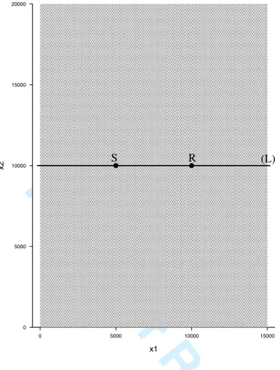
Let us turn now to a practical application of the homogenization theory in a periodic setting. A numer-ical experiment is led in a rectangular plane (see Fig. 2) of size 15 × 20 km2, surrounded by absorbing
boundary layers (which is not important here, for the sole balistic arrival is of interest, the coda waves being non-existent). The microscopic structure is that of a stretched checkerboard, as shown in Fig. 1, with a horizontal periodicity of 120 m, and a vertical one of 200 m. Elastic properties and density in the elements of the periodic cell, are ±50% around a mean value of 60 GPa for µ11and µ22(µ12being
null), and 2800 kg m−3for ρ.
To obtain values for the first-order corrector components and their spatial derivatives, the cell problem
1 2 3 4 5 6 7 8 9 10 11 12 13 14 15 16 17 18 19 20 21 22 23 24 25 26 27 28 29 30 31 32 33 34 35 36 37 38 39 40 41 42 43 44 45 46 47 48 49 50 51 52 53 54 55 56 57 58
For Peer Review
0 5000 10000 15000 20000 x2 0 5000 10000 15000 x1 S R (L)Figure 2. Periodic model. The periodicity vector is " = (%1, %2) = (120m, 200m). The point source is located
at S, the receiver at R. The (L)-line is the one along which are calculated snapshots shown in Fig. 4.
(27) is solved using periodic boundary conditions. The differential equations are solved with a finite element method based on the same mesh and quadrature than the one that will be used to solve the wave equation. This then allows to compute the homogenized stiffness tensor µ∗and density ρ∗, and the 0th-order homogenized wave equation,
$ρ% ∂ttu − ∇x· (µ∗· ∇xu) = f . (51)
using the spectral element method (SEM, see for instance Komatitsch & Vilotte (1998)).
The collocated source is located at S = (xS1, xS2) = (5 km, 10 km). Its time evolution is described
by a Ricker with a central time shift of 0.4 s and a central frequency of 5 Hz (to which is associated a corner frequency of about 12.5 Hz). A receiver is located at R = (xR1, xR2) = (10 km, 10 km),
therefore, at the same vertical component as the source, which means, that the periodicity seen at this receiver point, is of 120 m. Considering the physical properties of the medium (with a mimimum
1 2 3 4 5 6 7 8 9 10 11 12 13 14 15 16 17 18 19 20 21 22 23 24 25 26 27 28 29 30 31 32 33 34 35 36 37 38 39 40 41 42 43 44 45 46 47 48 49 50 51 52 53 54 55 56 57 58
For Peer Review
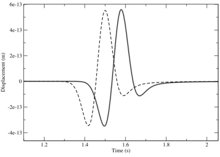
1.2 1.4 1.6 1.8 2 Time (s) -4e-13 -2e-13 0 2e-13 4e-13 6e-13 Displacement (m)Figure 3. Displacement (in meters) recorded at the receiver R located at (10km,10km). The reference is plotted
in grey, the order 0 homogenized solution in black, and the “natural averaging” (see text)solution is in dashed line.
wavelength of around 370 m), and the cut-off frequency of the source, the value of ε in the far field, is around 0.32. In order to properly compare the homogeneous solution with a reference one, calculated in the reference checkerboarding box, both solutions are computed with the same mesh (each element of this latter, corresponding to an element of the checkerboard), and the same time step (10−3s). The seismogrames resulting of these numerical simulations are reported in Fig. 3, in which are shown the reference solution (grey line), the order 0 homogenized solution (black line) and a solution obtained when taking the arithmetic average of both density and elastic constants (dashed line). Clearly, this last solution (which could be seen as a “natural averaging” solution) is not in phase with the reference one, whereas there is an excellent agreement between this latter, and the order 0 homogenized seismogram. Snapshots along a line (L) (see Fig. 2) between the source and the receiver, are shown in Fig. 4.a for each of the simulations, at t =0.4 s. Once again, the agreement is excellent between reference and 0th-order homogenized solutions, and very poor with the “natural filtering” solution.
The residual between the reference solution and the order 0 homogenized solution uε(x, t) − ˆu0(x, t), at t =0.4 s, is plotted in Fig. 4.b. The error amplitude is lower than the percent and contains fast variations.
Once done the 0th order homogenized simulation (and therefore, once known displacement gradients),
1 2 3 4 5 6 7 8 9 10 11 12 13 14 15 16 17 18 19 20 21 22 23 24 25 26 27 28 29 30 31 32 33 34 35 36 37 38 39 40 41 42 43 44 45 46 47 48 49 50 51 52 53 54 55 56 57 58
For Peer Review
we can compute the incomplete order 1 solution (49), again, at any time after the source excitation. In Fig. 4.c is shown the partial order 1 residual uε(x, t) − ˆu1/2(x, t). Comparing Fig. 4.b and Fig. 4.c,
it appears that the partial order 1 periodic correction removes most of the fast variations present in the order 0 residual. The remaining fast variations are due to the neglected higher-order terms, in the expansion (48). The smooth remaining residual could be due to'u1( term (and also, to higher-order
ones in 47) that is (are) not computed. In order to check the order of that this smooth remaining residual, we perform a test similar (at t =1.2 s) to the previous one, but with ε = 0.16 (which corresponds to a periodicity divided by a factor 2). Surprisingly, there is approximately a factor 4 in amplitude between both (see Fig. 4.d), which indicates a residual of order ε2, almost. That means that the'u1( term is quite close to being null; probably because the coefficients of µ1∗are quite small in
(45) - homogenized elastic properties in the unit cell, are close to being isotropic, which is in fact the case - and that (45) can be rearranged as in Capdeville et al. (2009a) ('u1( being equal to 0 in 1D).
3 NON PERIODIC CASE
Let us now turn to the case of interest in geophysics: the Earth material properties being not spatially arranged periodically, we give up this drastic hypothesis and consider more complex patterns for het-erogeneities - more precisely: we do not make any assumption on the spatial variability of density and elastic coefficients. After a theoretical treatment, we will apply it to the specific case of a plane in which properties are randomly generated around a constant mean value, as in Capdeville et al. (2009b), surrounded by a strip of progressively constant physical properties (to avoid any spurious reflection) and a PML (Perfectly Matched Layers, e.g. Festa & Vilotte (2005)) layer (to avoid the treatment of boundary layers in our homogenization procedure), as shown in Fig. 5.a. Note that this problem we shall tackle, is not that of the homogenization of random structures as studied by Papanicolaou & Varadhan (1979); in our example, the properties will be spatially known and unique.
Obviously we will still assume a minimum wavelength λm(or a maximum wave-number km = 1/λm)
for the anti-plane wavefield u, far enough from the source. Therefore, to some sense, heterogeneities in the plane, whose the size is much smaller than λm, should have a little, effective influence on the
wavefield u and an homogenization procedure may be hopefully performed. As recalled by Aki & Richards (1980), there are 3 different wave propagation regimes (waves in a smoothly-varying body, coda waves, and the homogenized part of a wavefield) depending on the ratio of the wavefield charac-teristic scale, to the one of the heterogeneities.
But when properties are not periodic in space: what is the characteristic scale of the heterogeneities? The whole difficulty we are faced to, is therefore to find a clear spatial scale delimitation (to apply an homogenization procedure), in order to catch wavefield properties in each of these regimes. In 1D,
1 2 3 4 5 6 7 8 9 10 11 12 13 14 15 16 17 18 19 20 21 22 23 24 25 26 27 28 29 30 31 32 33 34 35 36 37 38 39 40 41 42 43 44 45 46 47 48 49 50 51 52 53 54 55 56 57 58
For Peer Review
10000 11000 12000 13000 14000 x1 (m) -2e-13 0 2e-13 4e-13 Displacement (m) (a) 10000 11000 12000 13000 14000 x1 (m) -6e-15 -4e-15 -2e-15 0 2e-15 4e-15 Displacement (m) (b) 10000 11000 12000 13000 14000 x1 (m) -4e-15 -2e-15 0 2e-15 4e-15 Displacement (m) (c) 12000 12500 13000 13500 14000 14500 15000 x1 (m) -6e-15 -4e-15 -2e-15 0 2e-15 4e-15 (d)Figure 4. -a: grey line: snapshot of the displacement uε(x, t) at t =0.4 s computed in the reference model.
Black line: the order 0 homogenized solution ˆu0
(x, t). Dashed line: solution computed in a model obtained by arithmetically averaging the elastic properties.
-b: order 0 residual, uε(x, t) − ˆu0
(x, t). -c: partial order 1 residual, uε(x, t) − ˆu1/2,ε
(x, t).
-d: grey line: partial order 1 residual for ε = 0.32. Black line: partial order 1 residual for ε = 0.16 with an amplitude multiplied by 4, at t =1.2 s .
Capdeville & Marigo (2007) suggested to apply a filter to the recast elastic operator in the frequency domain, or to some physical quantities known a priori (Capdeville et al., 2009a); this filtering op-eration allowed them to obtain very accurate “homogenized” solutions, when compared to reference ones. Unfortunately, in a most general case, we do not know to which physical quantities this filtering procedure has to be applied. We will suggest one way to proceed (as done in Capdeville et al. (2009a)),
1 2 3 4 5 6 7 8 9 10 11 12 13 14 15 16 17 18 19 20 21 22 23 24 25 26 27 28 29 30 31 32 33 34 35 36 37 38 39 40 41 42 43 44 45 46 47 48 49 50 51 52 53 54 55 56 57 58
For Peer Review
after having recalled some filtering notions, and having set up a heuristic homogenization procedure to wave propagation in 2D non-periodic domains.
3.1 Basic notions on spatial filtering
In the theoretical development that will follow, we shall desire to separate low from high wave-numbers k = 1/λ (the norm of the wavenumber vector k) of a spatial distribution of any given quantity g(x) (which can be a tensor of any order), around a given wavenumber k0. Note that the
choice of k0 will be determinant to accurately described waveform properties in each propagation
regime.
To that purpose we shall introduce a low-pass space filter operator that takes the form, for any function g: Fk0(g) (x) = & R g(x$)wk0(x − x $)dx$, (52)
where wk0 is a wavelet that would ideally be defined in the spectral domain as
¯ wk0(k) = 1 for k ≤ k0; 0 for k > k0, (53)
where ¯w is just the Fourier transform of w.
In practice, in order to have a wavelet wk0 for which a compact support is a good approximation, we
do not use a filter with such a sharp cutoff but one defined by a smoother transition from 1 to 0 around k0. There are many ways to design a filter with such a property. The one we shall use is characterized
as: ¯ w(k) = 1 for k ≤ kmin; 1 2 -1 + cos-π |k|−kmin kmax−kmin ..
for |k| ∈]kmin, kmax[ ;
0 for |k| ≥ kmax.
, (54)
where kmin and kmax are two real numbers around 1, defining for the low pass filter the tapering
zone from 1 to 0. Just notice that the following property is verified: 3
R2w(x)dx = 1, and that we
can easily define wk0(x) = k0w(xk0), the same but contracted (if k0 > 1) wavelet of corner spatial
frequency k0, that also verifies:
3
R2wk0(x)dx = 1. The choice of kminand kmaxis ad hoc and left to
the user, this latter being aware of these 2 limitations: the perfectly sharp cutoff (kmin= kmax = 1) is
characterized by an infinite support in the space domain, that can not be truncated with a convenient accuracy; and any other choice, for which this truncation can be safely applied, does not present the interesting property of a perfectly clear separation of scales for a given quantity g.
1 2 3 4 5 6 7 8 9 10 11 12 13 14 15 16 17 18 19 20 21 22 23 24 25 26 27 28 29 30 31 32 33 34 35 36 37 38 39 40 41 42 43 44 45 46 47 48 49 50 51 52 53 54 55 56 57 58
For Peer Review
3.2 Set up of the homogenization problem in the nonperiodic case
In 1D, Capdeville et al. (2009a) applied the previous filtering operation to physical quantities that were explicitly known a priori. For wave propagation in higher dimensions, we do not have access to this kind of information, and do not know how to separate scales for density and elastic constants, in order to proceed to an homogenization of these quantities and of the wave equation. In other words, we do not know, for a given distribution of material properties, how to construct the x and y contributions of ρ and µ, from ρ0 and µ0. To that purpose, we then present here, an original but heuristic procedure. Classically a small parameter ε is introduced to solve the so-called two-scale homogenization prob-lems:
ε = λ λm
, (55)
where λ is a spatial wavelength, upon which will depend our asymptotic expansion (see below). For a periodic medium, λ would be the local length defining the periodicity of the model (called % in the first section of this article). In the non periodic case, it is not as obvious (because of the absence of an isolated characteristic length), and the introduction of another parameter is required
ε0=
λ0
λm
. (56)
λ0 is the length below which a wavelength can be considered as belonging to the small scale
(mi-croscopic) domain, and reciprocally for the large (or ma(mi-croscopic) scale. This λ0-parameter can be
arbritrarily chosen; nevertheless it makes sense to assume that the wavefield does interact with hetero-geneities whose size is smaller than λm. Therefore, picking a ε0 << 1, which means considering as
microscopic, heterogeneities whose size is much smaller than the minimum wavelength, should be a good guess.
Exactly as done in the periodic case, we can now introduce the fast space variable y = x/ε, treat x and y as independent space variables when ε tends towards 0, and redefine the gradient operator as in (7).
We then introduce a wavelet wm(y) = wkm(y) where wkm is a low-pass filter as defined in 3.1 and
km = 1/λm. We obviously assume that we can design it in such a way that its support in the space
domain is contained in an interval [−αλm, +αλm]2, where α is a positive real number.
Let Y0 = [−βλm, βλm]2 be a square of R2, with β a positive real number much larger than α,
and Yx the same square, but translated by a vector x/ε0. We define T = {g(x, y) : R2 × Y0 →
R , Y0-periodic in y} the set of functions defined in y on Y0and extended to R2by periodicity.
As-sociated to the wavelet wm, can be defined a filtering operator for any function g ∈ T :
F (g) (x, y) = & R2 g(x, y$)wm(y − y$)dy$. (57) 1 2 3 4 5 6 7 8 9 10 11 12 13 14 15 16 17 18 19 20 21 22 23 24 25 26 27 28 29 30 31 32 33 34 35 36 37 38 39 40 41 42 43 44 45 46 47 48 49 50 51 52 53 54 55 56 57 58
For Peer Review
Finally let V be the set of functions g(x, y) such that, for a given x, the y part of g is periodic and contains only spacial frequencies higher than km, plus a constant value in y:
V = {g ∈ T /F (g) (x, y) = $g% (x)} , (58)
where, similarly to the periodic case, the cell average of g over the newly defined periodic cell is $g% (x) = 1
|Y0|
&
Y0
g(x, y)dy . (59)
Of course, as in our procedure to treat wave propagation in nonperiodic media, the periodicity con-dition is kept, properties (11) and (13) are still valid. Furthermore, it is easy to show that, for any (tensorial) function g in V, the (spatial) partial derivatives of its components are also in V, and finally that:
∀h ∈ V with $h% = 0 and ∇g = h ⇒ g lies in V . (60) In this section and the next one, we proceed in the same way as in Capdeville et al. (2009a). We first assume that we have been able to define (ρε0(x, y), µε0(x, y)) that verify
ρε0(x, x/ε
0) = ρ0(x)
µε0
(x, x/ε0) = µ0(x)
(61)
and that set up a sequence (as in the periodic case) of models indexed by ε ρε0,ε(x) ≡ ρε0(x,x ε) , µε0,ε (x) ≡ µε0 (x,x ε) . (62)
We also guess that, with such a set of parameters, a solution to the homogenization problem described below exists. This is by far not obvious. The construction of such (ρε0(x, y) and µε0(x, y)) from
(ρ0(x) and µ0(x)), which is therefore a critical issue, is left for section 3.4.
As in the periodic case (and after recasting of the wave equation, see appendix A), we then look for the solutions of the wave equation and constitutive relation
ρε0,ε ∂ttuε0,ε− ∇ · σε0,ε = f , σε0,ε = µε0,ε · ∇uε0,ε . (63)
A solution to the equations (63) is again sought as an asymptotic expansion in ε: uε0,ε (x, t) = ∞ % i=0 εiuε0,i (x, x/ε, t) = ∞ % i=0 εiuε0,i (x, y, t) σε0,ε(x, t) = ∞ % i=−1 εiσε0,i(x, x/ε, t) = ∞ % i=−1 εiσε0,i(x, y, t) , (64) 1 2 3 4 5 6 7 8 9 10 11 12 13 14 15 16 17 18 19 20 21 22 23 24 25 26 27 28 29 30 31 32 33 34 35 36 37 38 39 40 41 42 43 44 45 46 47 48 49 50 51 52 53 54 55 56 57 58
For Peer Review
with the additional hypothesis - in this specific, nonperiodic case -, that uε0,iand σε0,imust belong to
the space V. Introducing the expansions (64) in the wave equations (63) and using (7) we obtain the system of differential equations
ρε0
∂ttuε0,i− ∇x· σε0,i− ∇y · σε0,i+1= f δi,0 (65)
σε0,i= µε0·)∇uε0,i+ ∇uε0,i+1* , (66)
which need to be solved for each i, up to a given i0. As in the periodic case (section 2.4), we will
restrict this resolution to order 1/2, that means: i0= 0, plus the first-order periodic correction.
3.3 Resolution of the two scale homogenization problem
We follow the same procedure as for the periodic case. We work at ε0. Because the y periodicity is
kept in V, the resolution of the homogenized equations is almost the same as in the periodic case. The major difference is that each physical quantity we look for, depends on ε0and on x.
• As for the periodic case, equations (65) for i = −2 and (66) for i = −1 give σε0,−1 = 0 and
uε0,0 ='uε0,0( (x).
• Equations (65) for i = −1 and (66) for i = 0 give ∇y· σε0,0
= 0 , (67)
σε0,0
= µε0
· (∇yuε0,1+ ∇xuε0,0) . (68)
Both previous equations lead to this next equality: ∇y·)µε0 · ∇
yuε0,1* = −∇y·)µε0· ∇xuε0,0* , (69)
Similarly to the periodic case, we can look for a solution of the form uε0,1
(x, y) ='uε0,1( (x) + χε0,1
(x, y) · ∇xuε0,0(x) . (70)
As uε0,1must belong to V, and because uε0,0is y-independent, the first order corrector χε0,1(x, y)
(a vector of dimension 2) must also be in V. We will see in section 3.4, how to proceed to obtain a first-order corrector that has this property. Introducing (70) into (69), we obtain the equations of the cell problems: ∇y· -µε0 ·-∇yyk+ ∇χε0,1 k .. = 0 . (71)
To enforce the uniqueness of the solution, we again impose4χε0,1
k
5 = 0. As in the periodic case, we can rewrite (71) under the equivalent form ∇y· Hε0 = ∇y· (µε0· Gε0) = 0 , (72) 1 2 3 4 5 6 7 8 9 10 11 12 13 14 15 16 17 18 19 20 21 22 23 24 25 26 27 28 29 30 31 32 33 34 35 36 37 38 39 40 41 42 43 44 45 46 47 48 49 50 51 52 53 54 55 56 57 58
For Peer Review
with Hε0 = µε0 · Gε0, and Gε0 = I + ∇χε0,1, where I is the unit tensor.Taking the cell average of (68) and using the ansatz (70), together with the guess that the first-order corrector can be found in V, we obtain the order 0 homogenized constitutive relation:
'σε0,0( = µε0∗
· ∇xuε0,0, (73)
where µ∗ε0 is the order 0 homogenized elastic tensor whose components again are (as in the periodic
case): µ∗ε0 ij = 4 µε0 ik(δjk+ ∂yjχ ε0,1 k ) 5 . (74)
As in the periodic case, it is easy yo show the following equality µ∗ε0
= $Hε0
% , (75)
and also that σε0,0
= Hε0
· ∇uε0,0
, (76)
Obviously, because we look for σε0,0belonging to this space, Hε0 mus lie inV. Furthermore, as it is
needed - to obtain the desired asymptotic solution of our problem- that the first-order corrector also be in this space, Gε0
, and because it is its gradient, must lie in V. These remarks will be fundamental, in our quest of the construction of a suitable µε0(x, y) in section 3.4.
• Finally, equation (65) for i = 0 gives ρε0∂
ttuε0,0− ∇x· σε0,0− ∇y· σε0,1= f . (77)
To be able to obtain σε0,1in V, the last equation implies that ρε0 must lie in V. Taking the average of
this equation, together with (68) leads to the order 0 homogenized wave equation $ρε0
% ∂ttuε0,0− ∇x· σε0,0= f (78)
'σε0,0( = µ∗ε0· ∇
xuε0,0. (79)
As we have seen for the periodic case, pushing the development further, leads to effective equations that are not those implemented in the spectral elements’ codes. Furthermore, and more dramatically, in 1D (Capdeville et al., 2009a), a nonperiodic development as the one looked for in this article, is only valid for the order 0 and the first order corrector. It is valid for higher order only in certain specific cases. Therefore, we do not go further, and again looks for a partial first-order solution, as in the section of this article, dedicated to periodic settings. As for the periodic case, the different orders can be combined as shown in section 2.4. For our partial first-order solution, and using the same notations,
1 2 3 4 5 6 7 8 9 10 11 12 13 14 15 16 17 18 19 20 21 22 23 24 25 26 27 28 29 30 31 32 33 34 35 36 37 38 39 40 41 42 43 44 45 46 47 48 49 50 51 52 53 54 55 56 57 58
For Peer Review
we then have ˆ uε0,ε,1/2 (x) =' ˆuε0,ε,0( (x) + χε0,1 (x, x/ε) · ∇x' ˆuε0,ε,0( (x) , (80)where the 1/2 superscript again means “partial order 1”. Of course, for it is only a partial order 1 solution, we do not have in general
uε0,ε
(x) = ˆuε0,ε,1/2
(x) + O(ε2) , (81)
Let us notice finally, that practically, only the case where ε0 = ε is of interest, as underlined by
Capdeville et al. (2009a), because it is the only value of ε0 that leads to the solution of the reference
problem (see 61).
3.4 Construction of ρε0(x, y) and µε0(x, y)
Here we are at the heart of the problem: how to conveniently construct ρε0(x, y) and µε0(x, y), in
order for uε,0, uε,1and σε,0 to be in V? As already said, µε0 must be built such that the first order
corrector χε0,1 (equation 70) and the vector Hε0 (equation 76) belong to V. Let us just recall that
χε0,1being in V implies that Gε0 also is (because it is its gradient). We will show that the reciprocity
is verified.
We therefore look for ρε0(x, y) and µε0(x, y) such that
(i) ρε0, Hε0 and χε0,1are in V;
(ii) ρε0 and µε0 must be positive definite;
(iii) ρε0(x, x/ε
0) = ρ0(x) and µε0(x, x/ε0) = µ0(x).
Let us introduce a given, starting ρ0s(x, y) = ρ0(ε0y) defined on R × Yxand then y-extended
peri-odically to R2. Note that this starting density distribution, is x-dependent.
The construction of ρε0(x, y) is then trivial:
ρε0(x, y) = F)ρ0
s* (x, x/ε0) + (ρ0s− F)ρ0s*)(x, y) (82)
We indeed have ρε0(x, x/ε
0) = ρ0(x) and ρε0 is in V and is a positive function with a well chosen
wavelet wm.
It is by far not so easy to find a correct µε0. We shall follow the same procedure described in Capdeville
1 2 3 4 5 6 7 8 9 10 11 12 13 14 15 16 17 18 19 20 21 22 23 24 25 26 27 28 29 30 31 32 33 34 35 36 37 38 39 40 41 42 43 44 45 46 47 48 49 50 51 52 53 54 55 56 57 58
For Peer Review
et al. (2009a) or Capdeville et al. (2009b). Let us recall that these fields are defined as: Gε0 = I + ∇yχε0,1, (83) Hε0 = µε0· Gε0, (84) ∇y· Hε0 = 0 , (85) $Gε0 % = I . (86)
To find convenient G and H, we process in the following way:
(i) Step 1: at a given x, let us define the area Yx, and build a starting µε0,s(x, y) = µ0(x, ε0y) on
it. Then solve for the (starting) periodic corrector solution of (85) with periodic boundary conditions on Yx, in order to find χε0,1,s(x, y).
Then we can compute Gε0,s (x, y) = I + ∇yχε0,1,s, (87) Hε0,s (x, y) = µε0,s (x, y) · Gε0,s (x, y) . (88)
At this stage, we can already compute the effective elastic tensor for any x: µ∗,ε0
(x) =-F (Hε0,s
) · F (Gε0,s
)−1.(x/ε0) . (89)
(ii) Step 2: now let us compute for any y ∈ Yx,
Gε0 (x, y) = [(Gε0,s − F (Gε0,s )) (y)] · [F (Gε0,s ) (x/ε0)]−1+ I , (90) Hε0 (x, y) = [(Hε0,s − F (Hε0,s )) (y) + F (Hε0,s ) (x/ε0)] · [F (Gε0,s) (x/ε0)]−1 . (91)
The extension of Gε0 and Hε0 from Y
xto R2in y in then done by periodic extension. At this stage,
we can check that (H, G) ∈ V2, and that $G% = I.
This last property is interesting, because of the definition (83) of Gε0 and the fact that this
quan-tity belongs to V: it implies that ∇yχε0,1 also belongs to V; it has also the following property:
'∇yχε0,1( = 0, and then, because of (60) , we finally derive the necessary condition: χε0,1∈ V.
(iii) Step 3: From (84) we can now build µε0(x, y) =
-Hε0· (Gε0)−1
.
(x, y) , (92)
(iv) Step 4: once µε0(x, y) is known, the whole homogenization procedure can be pursued to find
the different components of the 1st-order corrector vector.
This procedure may seems obscure and here is a tentative of interpretation (that is a bit different than the one given in Capdeville et al. (2009a) or Capdeville et al. (2009b)). The idea behind step one, is to first assume that all scales are fast. Then, the cell problem equations (71) (which are those of the static
1 2 3 4 5 6 7 8 9 10 11 12 13 14 15 16 17 18 19 20 21 22 23 24 25 26 27 28 29 30 31 32 33 34 35 36 37 38 39 40 41 42 43 44 45 46 47 48 49 50 51 52 53 54 55 56 57 58
For Peer Review
equilibrium in mechanics) are solved. They describe the microscopic effect of the imposition of a unit gradient in displacement in the yk-direction: the associated (microscopic) displacement obviously is
yk+ χεk0,1,s; therefore Gε0,sonly is the gradient of this displacement (as equation (83) indicates) and
Hε0,s the microscopic stress associated to this gradient. The idea behind any elastic homogenization
technique, is to find the effective tensor that links an effective stress and an effective deformation: this is exactly what is done in equation (89) where F (Hε0,s) and F (Gε0,s) play the role of the effective
stress and deformation. Equation (89) allows to directly determinate (after filtering) the homogenized elastic tensor, without solving for the “correct” other quantities, with the starting µε0,s(y). Practically,
in order to ensure the symmetry of this effective elastic tensor, we impose, in this procedure, the equality of µ∗,ε0
12 and µ∗,ε
0
21 , adding then a condition in (89) and solving this latter using a singular
value decomposition. Steps 2 and 3 allow to build µε0(x, y) by separating the scales of Hε0,s and
Gε0,susing the filter F () and making sure that $Gε0% = I.
Following all these operations, we have by construction µε0(x, x/ε
0) = µ0(x) and µε0is positive
definite for a well chosen wavelet wm. We also have checked that χε0,1also belongs to V (we have
Gε0 ∈ V and $Gε0% = I by construction (see step 2), which, using (60), indeed implies that χε0,1
belongs to V ). This corrector is unique when we impose the classical averaging condition'χε0,1( = 0.
In order to determine χε0,1, we first find µε0 with (92) and solve (71) once again.
As noticed by Capdeville et al. (2009b), we are not yet able to prove the symmetry of the homogeneous elastic tensor µ∗,ε0 in the general case, using the procedure presented in this section. We prove it in
the specific case of a nonperiodic but layered medium, in appendix C.
3.5 Homogenization in a non-periodic setting: an example
To validate it, we finally apply the homogenization procedure developed previously, for wave propa-gation throughout the random model shown in Fig. 5-a. This model is a square of size 20 × 20 km2,
surrounded by a 1km thick strip of constant physical properties (µ011 = µ022 = 60 GPa, µ012 = µ021 = 0GPa, ρ = 2800 kg m−3), plus an additional PML to avoid reflections at the boundaries in long-time simulations. This square is divided in elements of size 100×100m2. Elastic values in each element are randomly generated within ±50% of the elastic values of the surrounding strip; note that it is decided to start with an isotropic model, so the reference values for µ0
11and µ022are equal.
A reference solution can be computed in this model using SEM. A collocated source is located at S = (xS1, xS2) = (100 m, 10 km). Its time evolution is described by a Ricker with a central time shift
of 0.4 s and a central frequency of 5 Hz (to which is associated a corner frequency of about 12.5 Hz). Seismograms are recorded at fourteen receivers as shown in Fig. 5-a. A seismogram recorded at re-ceiver 8, and resulting of such a numerical simulation, is reported in the different collection of traces
1 2 3 4 5 6 7 8 9 10 11 12 13 14 15 16 17 18 19 20 21 22 23 24 25 26 27 28 29 30 31 32 33 34 35 36 37 38 39 40 41 42 43 44 45 46 47 48 49 50 51 52 53 54 55 56 57 58
For Peer Review
0 10000 20000 x2 0 10000 20000 x1 30 40 50 60 70 80 90 C11 (GPa) S 1 2 3 4 5 6 7 8 9 1011121314 0 10000 20000 x2 0 10000 20000 x1 30 40 50 60 70 80 90 C11 (GPa)Figure 5. a- Square, random model. The point source is located at S, the 14 receivers are also indicated. Here
are represented the values of the µ0
11coefficient.
b- Homogenized (or effective) model for the square, random model. On this figure are reported the values for the homogenized coefficient µ∗,ε0
11 , with ε0equal to 0.27. 8 9 10 11 x1 (km) 50 55 60 65 70 Stiffness (GPa)
Figure 6. Portion of a one-dimensional section, at x2 = 10km, of the stiffness µ 0
11 in the original, random
model (black line) and in its homogenized, effective counterpart ((µ∗,ε0
11 , in dashed grey line). Here ε0is equal
to 0.54. 1 2 3 4 5 6 7 8 9 10 11 12 13 14 15 16 17 18 19 20 21 22 23 24 25 26 27 28 29 30 31 32 33 34 35 36 37 38 39 40 41 42 43 44 45 46 47 48 49 50 51 52 53 54 55 56 57 58
For Peer Review
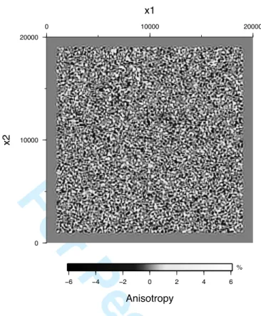
0 10000 20000 x2 0 10000 20000 x1 −6 −4 −2 0 2 4 6 Anisotropy %Figure 7. Effective anisotropy for the random model, calculated as (µ∗,ε0
11 − µ∗,ε
0
22 )/µ∗,ε
0
11 , with ε0=0.27.
in Fig. 8, in grey line with black dots.
As for the homogenization, and practically, we first solve the cell problem (71) on small domains YX, with periodic boundary conditions, for a large number of x-values. We therefore obtain values
for first-order correctors and for homogenized coefficients. The resolution of the cell problem is done using a finite element method, based on the same mesh and quadrature as the ones that is used in wave propagation simulations with SEM. In the following example, the polynomial order of the expansion of physical fields, is equal to 4.
In Fig. 5-b is shown the effective model corresponding to the previous random model Fig. 5-a; it is ob-tained by applying a homogenization procedure with a low-pass filter whose the cut-off corresponds to a ε0equal to 0.27. As can be seen, elastic quantities also show rapid spatial variations, but these
varia-tions are much smoother than in the original medium. This can be seen more precisely along a section, see Fig. 6. It is also possible to determinate the apparent anisotropy, as seen by the wavefield whose the smallest wavelength is much larger than the characteristic size of the (isotropic!) heterogeneities; here we decide to measure the anisotropy as the normalized difference between the homogenized values for µ011and µ022: (µ∗,ε0
11 − µ ∗,ε0
22 )/µ ∗,ε0
11 (the other terms of the homogenized elastic tensor being very
1 2 3 4 5 6 7 8 9 10 11 12 13 14 15 16 17 18 19 20 21 22 23 24 25 26 27 28 29 30 31 32 33 34 35 36 37 38 39 40 41 42 43 44 45 46 47 48 49 50 51 52 53 54 55 56 57 58
For Peer Review
5 Time (s) -5e-12 0 5e-12 1e-11 Velocity (m/s) (a) 5 Time (s) -5e-12 0 5e-12 1e-11 Velocity (m/s) (b) 5 Time (s) -5e-12 0 5e-12 1e-11 Velocity (m/s) (c) 5 Time (s) -5e-12 0 5e-12 1e-11 Velocity (m/s) (d)Figure 8. Velocity traces computed for the collocated source S, at the receiver 8. The reference solution is in
grey with black dots; the order 0 homogenized solution, in black. The ε0-parameter takes values 2.16 (a), 1.08
(b), 0.54 (c) and 0.27 (d).
close to be null). As can be seen on Fig. 7, the anisotropy can be quite large, varying between -6% and 6%, with (absolute) average values lying between 1 and 2%. In Fig. 8 we compare the particle velocity (recorded at receiver 8, with the source located at S; see 5-a), calculated in the reference medium (grey line with black dots), to the one obtained with the sole order 0 homogenization ( ˙uε0,0), for different
values of ε0, varying from 2.16 to 0.27 (black line). For large values of ε0, that means, when the
ho-mogenized model is too smooth with respect to the minimum wavelength of the wavefield, it clearly appears that the coda of direct waves is nonexistent or incorrectly calculated. The more ε0 decreases,
the more the coda correctly “built” is: for a ε0of 0.27, the agreement between the reference and the
homogenized solutions, is excellent. Note that the arrival time of the ballistic wave is always rightly retrieved, whatever the value of ε0is; this is not the case when seismograms are recorded in effective
1 2 3 4 5 6 7 8 9 10 11 12 13 14 15 16 17 18 19 20 21 22 23 24 25 26 27 28 29 30 31 32 33 34 35 36 37 38 39 40 41 42 43 44 45 46 47 48 49 50 51 52 53 54 55 56 57 58
For Peer Review
5 Time (s) -5e-12 0 5e-12 1e-11 Velocity (m/s)Figure 9. Velocity traces recorded at the receiver 8 (see Fig. 5-a). The reference solution is plotted in grey, and
the “natural filtered” solution is in dashed line. Both are clearly out-of-phase.
media when a simple (and erroneous) filtering is applied to elastic quantities (see Fig. 9).
Let us now take a look at the convergence of the homogenized solution uε0,0towards the reference
one uref. As suggested in the companion paper (Capdeville et al., 2009b), let us introduce a measure of the error between a given field u and the reference one, at a given receiver k, as:
Ek( ˙u) =
6 320
0 ( ˙u − ˙uref) 2 (xk, t)dt 6 320 0 ( ˙uref) 2 (xk, t)dt , (93)
where the maximal bound for the time integral, indicates that seismic recordings of interest last 20 seconds (after that time the amplitude of the coda wave is completely negligible). Then a combined error Etotcan be defined, taking into account the error at each individual receiver (see Fig. 5-a), as:
Etot( ˙u) = 1 14 14 % k=1 Ek( ˙u) . (94)
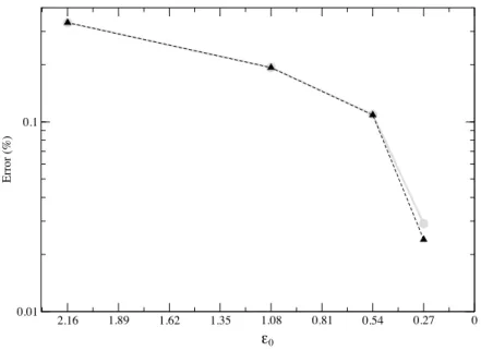
As in the P-SV case (Capdeville et al., 2009b), the error Etot( ˙uε0,0) decreases quite slowly when ε0
with large values, decreases (see Fig. 10). The reason is quite obvious when taking a look at Fig. 8: the coda only begins to be fully constructed for values of ε0around 0.5. Quite surprinsingly, from this
point, the convergence is then very fast: instead of a theoretical, expected convergence in ε0, the order
0 homogenized converges towards the reference one, in ε20. For this random example, this observation
1 2 3 4 5 6 7 8 9 10 11 12 13 14 15 16 17 18 19 20 21 22 23 24 25 26 27 28 29 30 31 32 33 34 35 36 37 38 39 40 41 42 43 44 45 46 47 48 49 50 51 52 53 54 55 56 57 58
For Peer Review
0 0.27 0.54 0.81 1.08 1.35 1.62 1.89 2.16 0.01 0.1 Error (%) ε0Figure 10. Total error as defined in (94), as a function of ε0, between the order 0 homogenized solution
(E(uε0,0), straight line) or the partial first-order solution (E(uε0,1/2), dashed line), and the reference one.
underlies the fact that high-order terms in the asymptotic expansion (64) are negligible in comparison with the leading term. This is confirmed when calculating the same kind of error, but this time between the partial first-order solution uε0,1/2and the reference one (see Fig. 10): the effect of the correction
term is null for large values of ε0, and quite weak for small ε0s - even if clearly observable. Note that
Capdeville et al. (2009b) pursue the same kind of calculations for smallest values of ε0, for which the
effect of the first-order correction, is more pronounced. Finally, we observe a quite good convergence even for high ε0 values, because even if the source is located in a homogeneous zone, the area on
which we calculate correctors and homogenized quantities, is larger than the homogeneous, surround-ing strip of the box model (see Fig. 5) when ε0is equal to 2.16, therefore the first-order correction for
the point source (see Capdeville et al. (2009a)) should be taken into account in this case (and the error associated with this large ε0 should then be lower than the one calculated here).
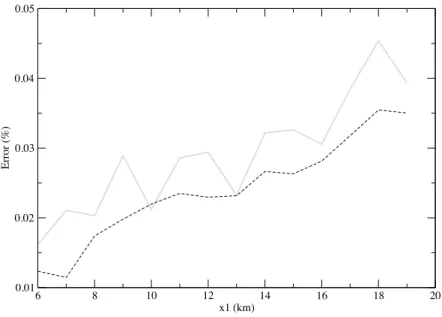
The effect of the first-order correction can be observed in Fig. 11, where are reported the errors E( ˙uε0,0) and E( ˙uε0,1/2) as a function of x
1, along a line joining all receivers plotted on Fig. 5-a.
The error almost always decreases with the supplemented corrective first-order term. We also observe, although it is less marked than in the P-SV case, that the error determined for the partial first-order homogenized solution, varies more slowly with x1, than the one for the order 0 solution. This effect
can be explained by the fact that the first-order corrector term, depends on y (fast scale)- and then
1 2 3 4 5 6 7 8 9 10 11 12 13 14 15 16 17 18 19 20 21 22 23 24 25 26 27 28 29 30 31 32 33 34 35 36 37 38 39 40 41 42 43 44 45 46 47 48 49 50 51 52 53 54 55 56 57 58