A study of the robustness of the group scheduling method using an emulation of a complex FMS

HAL Id: hal-01115937

http://hal.univ-nantes.fr/hal-01115937

HAL is a multi-disciplinary open access archive for the deposit and dissemination of sci-entific research documents, whether they are pub-lished or not. The documents may come from teaching and research institutions in France or abroad, or from public or private research centers.

L’archive ouverte pluridisciplinaire HAL, est destinée au dépôt et à la diffusion de documents scientifiques de niveau recherche, publiés ou non, émanant des établissements d’enseignement et de recherche français ou étrangers, des laboratoires publics ou privés.

A study of the robustness of the group scheduling

method using an emulation of a complex FMS

Olivier Cardin, Nasser Mebarki, Guillaume Pinot

To cite this version:

Olivier Cardin, Nasser Mebarki, Guillaume Pinot. A study of the robustness of the group schedul-ing method usschedul-ing an emulation of a complex FMS. International Journal of Production Economics, Elsevier, 2013, 146, pp.199 - 207. �10.1016/j.ijpe.2013.06.023�. �hal-01115937�

A study of the robustness of the group scheduling method using an emulation of a complex FMS Olivier Cardin a, Nasser Mebarkia, Guillaume Pinot a

a

LUNAM Université, IUT de Nantes – Université de Nantes, IRCCyN UMR CNRS 6597 (Institut de Recherche en Communications et Cybernétique de Nantes), 2 avenue du Pr Jean Rouxel – 44475 Carquefou

Corresponding Author : Olivier Cardin : olivier.cardin@irccyn.ec-nantes.fr;

Tel : +33 (0) 228092000 ; Fax : +33 (0) 228092021

Abstract

In the field of predictive-reactive scheduling methods, group sequencing is reputed to be robust (in terms of uncertainties absorption) due to the flexibility it adds with regard to the sequence of operations. However, this assumption has been established on experiments made on simple theoretical examples. The aim of this paper is to carry out experimentation on a complex flexible manufacturing system in order to determine whether or not the flexibility of the group scheduling method can in fact absorb uncertainties. In the study, transportation times of parts between machines are considered as uncertain. Simulation studies have been designed in order to evaluate the relationship between flexibility and the ability to absorb uncertainties. Comparisons are made between schedules generated using the group sequencing method with different flexibility levels and a schedule with no flexibility. A last schedule takes into account uncertainties whereas schedules generated using the group sequencing method do not. As it is the best possible schedule, it provides a lower bound and enables to calculate the degradation of performance of calculated schedules. The results show that group sequencing perform very well, enabling the quality of the schedule to be improved, especially when the level of uncertainty of the problem increases. The results also show that flexibility is the key factor for robustness. The rise in the level of flexibility increases the robustness of the schedule towards the uncertainties.

Keywords:Scheduling, Robustness, Flexibility, Group scheduling, Proactive-reactive scheduling.

1. Introduction

The most classical scheduling situation is the static scheduling, also called predictive scheduling. In this contextthe variables, theconstraints, the environment, all the data are considered as known. Then, the scheduling problem can be solved using combinatorial optimization methods, either exact methods such as linear programming, branch and bound methods, or heuristic methods (Pinedo, 2008).This phase is done off-line.

The problem is that manufacturing systems are not so deterministic. They present a lot of uncertainties and randomness, e.g., the breakdown of a machine, late material, new orders to proceed immediately, etc. During the execution of the schedule, it is frequently necessary to repair the schedule while preserving the solution’s quality. This phase is done on-line and is called reactive

scheduling or predictive-reactive scheduling since the reactive phase is based on a schedule computed during the predictive phase. When the schedule in progress can no longer be repaired, it is necessary to set a new predictive schedule.

Moreover, the model used to generate a schedule during the predictive phase can be more or less precise in regards with the real system (e.g. operating times considered as random, transfer times considered as negligible, etc.). Roy (2005) talks about “just about or ignorance areas that affect the modeling of a problem”.

To cope with these drawbacks, one can use real-time control methods (Chan et al., 2002). These kind of methods do not make any plan and builds the schedule dynamically. Generally, these methods use priority rules which determine for each resource of the shop the next operation to proceed among the waiting operations in the resource's queue. These methods consider the real-state of the shop, so hazardous phenomena can be effectively taken into account when they occur. As these methods deal with the real-state of the system, they are called reactive methods. The major drawback of the reactive methods is that their performance is generally poor.

Very few methods try to combine the advantages of both predictive and reactive methods. The proposed methods rely essentially on the introduction of slacks during the predictive phase in order to facilitate re-scheduling during the reactive phase. The idea is to introduce flexibility during the predictive phase in order to obtain a robust schedule, enabling to absorb the perturbations during its execution.This is called proactive scheduling (Herroelen and Leus, 2004; Van de Vonder et al., 2007). One of the most known proactivemethods in project scheduling is the critical chain method used in several project management pieces of software(Goldrath, 1997). The method relies on the introduction of slacks on the operations of the critical path in order to absorb the delays. Another proactive method is the Just In Case Scheduling method (Swanson et al., 1994). This method identifies the probable critical delays and for each of them an alternative scheduling is proposed.Other methods, using fuzzy logic, try to capture the uncertainties in the scheduling data.Caprihan et al. (2006) have added fuzzy criteria on priority rules such as Work In Next Queue (WINQ) and Number In Next Queue (NINQ). Domingos and Polianto(2003) have proposed a procedure for on-line scheduling where decisions are based on fuzzy logic.

In this paper, we focus on the group scheduling method which is one of the most studied proactive-reactive methods. This method is very interesting because it favors the cooperation between human and machine to address the uncertainties of both the system (i.e., randomness) and the model (i.e., lack of precision). This is done by defining a partial order of the operations on each machine, permitting the decision maker to complete the scheduling decisions according to his preferences and the real state of the shop. For this, the group scheduling method builds scheduling solutions that integrate sequential flexibility; moreover the method guarantees a minimal quality corresponding to the worst case. Thus, this method brings flexibility and enables to choose in real-time the operation (among a group of permutable operations) that fits best to the real state of the system However, group scheduling has a major drawback: when order groups are very large, the flexibility added to the schedule is bigger but the cycle times will be longer.

Group scheduling was first introduced in Erschler&Roubellat (1989). This method has been widely studied in the last twenty years, in particular in Erschler&Roubellat (1989), Billaut&Roubellat (1996), Wu et al. (1999) and Artigues et al. (2005).The flexibility added to the schedule should enable the

method to be robust, i.e. the method should absorb uncertainties, randomness and lack of precision of the model. Only two precedent studies have tried to verify this supposed property of the group scheduling method. Wu et al. (1999) study the impact of disturbed processing times on the objective of weighted sum of tardiness in comparison with static and dynamic heuristics. Esswein (2003) studies the impact of disturbed processing times, due dates and release dates on a one machine problem and compares its results with a static heuristic method.

Although these two studies show the capacity of group scheduling to be robust, they are made on simple and theoretical models with simplified assumptions.

This paper presents a new study to evaluate the capacity of group scheduling method to absorb uncertainties. Contrarily to previous studies done with the groupscheduling method, this study has been conducted on an emulation of a real flexible manufacturing system.As stated by Liu and MacCarthy(1996) a Flexible Manufacturing System (FMS) is an integrated system composed of automated workstations such as computer numerically controlled (CNC) machines with tool changing capability, a material handling and storage system such as automated guided vehicles or conveyors, and a computer control system which controls the operations of the whole system. It is frequently observed in the scheduling literature that transfer times are purely and simply ignored (Pinot, 2008). To evaluate the robustness of group scheduling in regards with uncertainties, we conducted experiments on a real FMS to test the effect of the non-consideration of transfer times in a predictive schedule. In order to have results on a large time horizon, experiments are made on an emulation of the real system and not directly on the real system.

The rest of the paper is organized as follows: first, the groupscheduling method is presented, second, the capacity of the group schedulingmethod to handle uncertainties are discussed, third, the different experiments made are presented, and finally the results, very promising, are discussed.

2. Group scheduling

Van de Vonder et al. (2007)propose a classification of scheduling methods under uncertainties. Their classification relies on the way uncertainties are taken into account. From this, they identity three major categories: proactive methods, reactive methods and proactive-reactive methods.

A proactive method is a method where flexibility is added in a predictive model in order to deal with the uncertainties when they occur. Its main advantage is that it permits the computation of an optimal solution of the schedule. The problem of this kind of methods is that it deals with a prediction of the system and not with the real state of the shop.

With reactive methods, decisions are taken considering the real events of the shop. So, these methods are really taking into account the uncertain nature of manufacturing systems. They are usually called dynamic methods because they build dynamically the schedule as one goes along the events in the system. Their main advantage is that they deal with the real-state of the shop but they may give poor solutions for the schedule.

Proactive-reactive methods deal with a static schedule computed by a predictive method during a first phase of the schedule called the predictive phase. Then, in a second phase re-schedulings are done in order to take into account the real-state of the shop. This second phase is called the reactive phase where the schedule is adjusted to the uncertainties which occur in the system. Thus, these

kinds of approaches are very interesting because they try to use the benefits of both predictive and reactive methods. Bel and Cavaillé (2001) describe different proactive-reactive methods.

One the most powerful and studied proactive-reactive methods is the group scheduling method. It is also one of the only proactive-reactive methods to be implemented in an industrialscheduling software named ORDOSoftware (Roubellat et al., 1995).

The group scheduling method was first introduced in (Erschler et al., 1989). The goal of this method is to provide a sequential flexibility during the execution of the schedule and to guarantee a minimal quality corresponding to the worst case. This method has been developed in the last twenty years, in particular in(Erschler et al., 1989), (Billaut et al., 1996), (Wu et al., 1999), (Artigues et al., 2005). A full theoretical description of the method is available in(Artigues et al., 2005). Let us describe the method and for this introduce some notations: in the rest of this article, the index i will be used for the operations and the index l will be used for the resources.

A group of permutable operations is a set of operations to be performed on a given resource Ml in an

arbitrary order. It is named gl,k. The group containing the operation Oi is denoted by g(i). The index k

will be used for the sequence number of a group.

A group sequence is defined as a sequence of vl groups (of permutable operations) on each machine Ml: gl,1, …, gl,vl, performed in this particular order. On a given machine, the group after (resp. before) g(i) is denoted by g+(i) (resp. g-(i)).

A group sequence is feasible if for each group, all the permutations among all the operations of the same group give a feasible schedule (i.e. a schedule which satisfies all the constraints of the problem). As a matter of fact, a group sequence describes a set of valid schedules, without enumerating them. The quality of a group sequence is expressed in the same way as that of a classical schedule. It is measured as the quality of the worst semi-active schedule found in the group sequence, as defined in (Artigues et al., 2005), where a semi-active schedule is a feasible schedule in which no local left-shift of an operation leads to another feasible schedule.

To illustrate these definitions, let us study an example.

Figure 1.A group sequence solving the problem described in Table 1.

Table 1 presents a job shop problem with three machines and three jobs, while Figure 1 presents a feasible group sequence solving this problem. This group sequence is made of seven groups: two groups of two operations and five groups of one operation. This group sequence describes four different semi-active schedules shown in Figure 1. Note that these schedules do not always have the same makespan: the best case quality is with Cmax = 10 and the worst case quality is with Cmax = 17.

Figure 2.Semi-active schedules described in Figure 1.

The execution of a group sequence consists in choosing a particular schedule among the different possibilities described by the group sequence. It can be seen as a sequence of decisions: each decision consists in choosing an operation to execute in a group when this group is composed of two or more operations. For instance, for the group sequence described on Figure 1, there are two decisions to be taken: on M1, at the beginning of the scheduling, either operation O1 or O8 has to be

executed. Let us suppose the decision taken is to schedule O1 first. On M3, after the execution of O7,

there is another decision to be taken: scheduling operation O3 or O5 first. If the decision is to execute O5 first, the first schedule of Figure 2 is realized.

Group scheduling has an interesting property: the quality of a group sequence in the worst case can be computed in polynomial time for minmax regular objective functions like makespan or maximum lateness (see (Artigueset al., 2005) for the description of the algorithm). Thus, it is possible to compute the worst case quality for large scheduling problems. Consequently, this method can be

used to compute the worst case quality in real time during the execution of the schedule. Due to this property, it is possible to use group scheduling in a decision support system in real time during the execution of the scheduling process.

To improve the performance of the group scheduling method, Pinot (2008), Riezeboset al. (2010) propose a complete study of the best case quality in a group schedule. The best case evaluation of a group schedule can be used during the predictive phase as well as during the reactive phase. During the predictive phase, the best possible performance of the schedule along with its worst case evaluation give the range of all possible performances of the future schedule. During the reactive phase, it can be used to assess possible decisions: one can know the best quality obtained if an operation is executed first, thus it allows better performance for the execution of the overall schedule.

The group scheduling method enables the description of a set of schedules in an implicit manner (i.e.,without enumerating the schedules). Actually, as it proposes a group of permutable operations, one can choose, during the reactive phase, inside a group the operation that best fits the real state of the system. For that, Thomas (1980) proposes an indicator called the sequential free margin which is a free margin adapted to group scheduling. The sequential free margin of a given operation represents the maximum tardiness that can be tolerated to guarantee no late jobs in every schedule described by the group sequence. This margin gives the ability to monitor the group sequence in real time: if the sequential free margin becomes negative, then some schedules described by the group sequence have late jobs. Such a margin is a very useful tool to take proper decisions and monitor the quality of the group sequence.

3. Robustness and group scheduling

A robust schedule can generally be defined as a schedule where perturbations are easily absorbed (Billaut et al., 2004). Thus, there is an association between flexibility and robustness, adding flexibility to a model is the way to have a robust schedule.

The goal of group scheduling is to propose sequential flexibility during the reactive phase of scheduling. This flexibility should improve the robustness of the method. Two studies evaluate the robustness provided by group scheduling: (Esswein, 2003) and (Wu et al., 1999).

Esswein (2003) formulates the predictive phase as a bi-objective problem: the first objective is the minimization of a regular objective (e.g., the makespan or the maximum lateness) in the worst case and the second is the maximization of the flexibility. The flexibility is expressed as a percentage according to the number of groups. A group sequence with a flexibility of 0% is a group sequence with one group per operation, and a group sequence with a flexibility of 100% is a group schedule with one group per machine. This flexibility represents the number of decisions to be effectively taken divided by the maximum number of decisions.

Esswein (2003) studies the robustness of group scheduling for one machine problems (1|ri, di|f) with

different objectives: Cmax (the makespan), Lmax (the maximum lateness), Tmax (the maximum tardiness) and ΣTi (the total tardiness). The study compares group scheduling with a static method. For the reactive phase, the free sequential margin proposed by Thomas (1980) is used to choose the operation in a group sequence. The static method is computed before the execution of the schedule using non disturbed data with the EDD priority rule.

Several types of uncertainties are studied: the increase of the release dates, the increase of the processing times and the decrease of the due dates. Several levels of perturbation are also tested. The results show that group scheduling is always better than the static method. In this study, adding flexibility at the expense of the worst case quality is generally profitable to the final quality of the schedule.

(Wu et al., 1999) uses group scheduling on a job shop with the minimization of the weighted total tardiness (J|| ΣwiTi). (Wu et al., 1999) call the method PFSL, but Artigues et al. (2005) have shown that this method is equivalent to group scheduling. The reactive phase uses priority rules to make the last decisions. This scheduling method is compared with a static method and a reactive method based on the ATC priority rule. The uncertainties studied are the variation of the processing times. The proposed scheduling method exhibits better performances when the uncertainties are small to moderated (p’i∈ [0.9pi, 1.1pi]).

This study shows that group scheduling can absorb uncertainties for small to moderated perturbed problems. This method does not use the free sequential margin, so group scheduling can be robust without this tool.

In both thestudies presented above, group scheduling exhibits better performance than static or dynamic methods when perturbations impact the execution of the schedule. At the end of hisstudy, Esswein (2003) conclude that if the results obtained are promising, the context of the experiment is limited and simple and the perturbations are limited as well. The same remarks can be made for the study of Wu et al. (1999). So, the question is “Do Group scheduling really absorbs uncertainties in a complex manufacturing system?” There is clearly a need for a detailed study to test the effectiveness of the robustness of the group scheduling method on a complexmanufacturing system.

According to Esswein (2003), « uncertainties describe potential modifications of some of the scheduling problem data which may occur between the computation of the schedule and the end of its execution in the shop ». Then,an uncertainty can be defined as a difference between the execution of a schedule and the hypotheses made for the computation of the schedule. Based on the classification proposed byRoy (2005), examples such as those could be addressed: rounding a length of a conveyor, difference of parameters in the orders compared to previsions, breakdowns and failures, lack of raw materials or inaccuracies in speeds and durations.

In this paper, we propose to test the robustness of the group scheduling method on an emulation of a real manufacturing system described below. This is a flexible manufacturing system modeled as a job-shop model. Frequently on job-shop models, the transportation system is not taken into account or whenever it is modeled, it is partially: only the transfertimes are modeled not the transport resources and their limited capacity. This assumption is very frequent on job-shop scheduling problems but not so trivial.Here, our assumption is to consider that the group sequence method is the right scheduling method to deal with a complex flexible manufacturing system without having a precise and complex job-shop model. The group sequence method is a proactive-reactive scheduling method. It means that as a proactive method, it introduces flexibility in the predictive schedule (i.e., groups of permutable operations) that should permit to give very good results during the execution of the schedule even if the job-shop model is approximate.

Our goal is to test the robustness of group scheduling with regards to uncertainties. In this study, the choice was made to choose, among all the possible uncertainties, thetransfer times. The main advantages of this choice are:

 It is possible to evaluate the exact impact of transfer time in the production, and thus find the optimal schedule using the same job-shop algorithm. This specificity is described later in this section when introducing the lower bound;

 It is possible to easily modify the impact of this uncertainty on the production by changing the speed of the transporters;

 This uncertainty is related to structural characteristics of the job-shop, which are thus static parameters of these experiments, therefore not chosen arbitrarily considering the scheduling problem.

In this section, we present in detail our experiments:

 To avoid the specificity of a single problem and thus biasing the results, 15 different scheduling problems were considered, each one with a 5 machines job shop and a various number of jobs., We have chosena set of benchmark instances called la01 to la15 from Lawrence (1984), used extensively in the scheduling literature. This set of instances is doubly useful: first it is a benchmark in the scheduling literature and second as optimal solutions with an approximation of transfer times can be computed, they will be used as lower bounds.

 The routings and the operating times of this set of instances will be used as input data for the FMS used in our study.

 In order to control the experiments and to reduce experiment times, the execution of the schedules on the production system were made through discrete-event simulation on an emulation of the real manufacturing system.

 The quality of the schedule is measured on the makespan. This performance criterion which measures the productivity of the system is one of the most used in the literature to evaluate the performance of scheduling methods (Buzacott and Yao, 1986, Chan et al., 2002, Pinedo, 2008). As the group scheduling method is implemented in an industrial software (ORDOSoftware), it is already used on real manufacturing systems and the performance measures usually used with ORDOSoftware are the makespan (i.e.,Cmax) and the maximum lateness (i.e.,Lmax). The makespan being the time difference between the start and finish of a sequence ofjobs, in our experiments the sequences of jobs were fixed and the initial and final states of the production system were considered as empty, in order to properly compare the different experiments.

 The production system is deterministic.

 Each schedule was executed 100 times on the simulated system, each execution with a different transportation speed. This was only possible because experiments were made on an emulation of the FMS and not directly on the FMS.

 To solve all the job-shop problems presented in this paper, we used the branch and bound algorithm described in Brucker et al. (1994). To generate the group sequences, we used a greedy algorithm (described in Pinot (2008) and Esswein (2003)) that merges two successive groups according different criteria until no group merging is possible without degrading the quality. This algorithm begins with a one-operation per group sequence from the schedule computed by the Brucker et al. (1994) algorithm used to solve the job-shop problems.

The next paragraphdescribes the construction of each schedule.

A lower bound, named LB, was computed. It is a solution of the classical job-shop scheduling problem with virtual machines added in order to model transportation times. This lower bound LB is compared to threedifferent schedules which are:

 NoTT (No Transfer Times): in this schedule, no transfer times are taken into account. By definition, this schedule will not allow any flexibility during the execution.

 OGSS (Optimal Group Sequence Schedule): in this schedule, the best case quality of the group sequence generated is equal to the worst case quality without any transfer times.  DGSS (Degraded Group Sequence Schedule): in this schedule, the worst case quality for the

scheduling problem without any transfer time is degraded. This group sequence offers more flexibility to choose operations during the execution of the schedule.

In order to conduct experiments on a large time horizon, we use an emulation (Pinot et al., 2007) of a Flexible Manufacturing System.The system under study (Fig. 3) is a Flexible Manufacturing System used as an experimental platform for research and teaching at the University of Nantes (France).

The system can be modeled as a six machines job shop, with automated transfers (Fig. 4). Each machine has a finite capacity upstream queue. Four of them are only FIFO queues, the two others enabling a free choice. Machine 6 is not considered in this study. Automated transfers between machines are performed by 42 unidirectional transporters, stored in a storehouse during the inactivity periods. They cannot handle more than one part at a time, but they also carry all data of the part updated in real-time (identification, routing, progress, etc.).

Figure 4.Job-shop model of the studied FMS.

The structure of the transport system is built around a central loop. Each transporter moves on the loop until it can enter the queue of a machine. To be more specific, when a transporter arrives at the entrance of any machine, a decision, based on the stock level, on the routing of the part and on the schedule of the machine, is made to allow (or not) the transporter to enter the queue of the machine. If not, the transporter goes ahead.

The emulation model allows us to simulate several scenarios, characterized by one parameter:the speed of the transporters (from zero to infinity).

Each transporter is assigned to a job at the exit of the storehouse, and is only freed when the job is completed. On the real system, these decisions are taken based on the data contained in the electronic tag of the transporter and the groups assigned to each station. Indeed, the schedules we suggest to work on can be implemented the same way, with the following specifications:

 each operation is assigned to a unique machine;

 for OGSS and DGSS, operations are stored in list of groups in each machine;

 forNoTT, each group has a single operation, thus there is no decision during the execution of the schedule.

As stated before, transportation times were chosen as the uncertainties considered in the model. Indeed, OGSS, DGSS and NoTT algorithms do not take into account the transportation times, and thus it is a disturbance in the execution of the schedule on the real system.As a matter of fact, changing the speed of the transporters enables to change the level of the uncertainties: the highest the speed of the transporters is, the less the uncertainties are.

Thus, to simplify the data analysis, we propose to use a parameter called the uncertainty degree and noted U°:

𝑈° = 𝑝𝑖 𝑙_𝑖,𝑗

With𝑝 the average processing time of an operation i and𝑙𝑖 the average transportation time between 𝑖,𝑗 two operations i and j.

As a consequence, U°= 1 means that processing times and transportation times are equal in average; U°= 10 means that transportation times are 10 times bigger than processing times in average; and U°= 0.1 means that processing times are 10 times bigger than transportation times in average. The model of the workshop was programmed with a discrete-event simulation tool, namely Arena. Its role is to exhibit the behavior of the real system (full of uncertainties) in response to a given schedule (not taking into account these uncertainties). A schedule is defined here as the output of the application of a scheduling algorithm to a scheduling problem. For each level of uncertainties, the transportation times evolve, and thus the problem is different.

For each schedule denoted Ψ, Ψ ∈ {LB, NoTT, DGSS, OGSS}, performance PΨ is measured as the total

makespan of the execution of the production.

For each Lawrence’s instance, the following happened:

1) 100 entry files E1 to E100 for the scheduler are generated introducing transfer times between each operation. Each file is different of the other because the speed is different, and thus the transfer times.

2) E1 to E100 are computed by the job-shop scheduler. The results represent the values of PLB.

3) An entry file E101 is generated, only considering the data from Lawrence’s instance (thus no transfer times).

4) The job-shop scheduler delivers a schedule S101 from E101.

5) 100 simulations are executed considering the schedule S101, each simulation with a different speed of the transporters. The results represent PNoTT.

6) The branch and bound algorithm delivers two schedules S102 and S103 from E101, S102 allowing a lower flexibility.

7) 100 simulations are executed considering the schedule S102, each simulation with a different speed of the transporters. The results represent POGSS.

8) 100 simulations are executed considering the schedule S103, each simulation with a different speed of the transporters. The results represent PDGSS.

As stated before, the emulation model was made deterministic, i.e. not considering any other disruptions than the transportation times. As a matter of fact, two consecutive simulations of the same schedule give the exact same result, which explain why no stochastic replications are made.

5. Results

PΨcan be considered as a function of the uncertainty degree U°, U°∈]0,+ ∞ [. Obviously, when U°

increases, every PΨ tends to increase in the same way. Therefore, in order to be able to compare the

results of each schedule, it was chosen to normalize the results in regards with the value of the Lower Bound (LB). This was made possible because LB was computedtaking into account the transfertimes.

In the following, the function obtained will be called the Degradation Function, as it measures the percentage of performance lost because of a non-optimal schedule. The degradation is computed as follows:

𝐷_𝜓 𝑈° =_𝑃𝑃𝜓 𝑈° 𝐿𝐵 𝑈° − 1

A couple of remarkable properties of D can be noted. By definition, we have: ∀𝑈° ∈]0; +∞[, 𝐷_𝐿𝐵 𝑈° = 0

As LB is a lower bound, we have:

∀𝑈° ∈]0; +∞[, 𝑃_𝜓 𝑈° ≥ 𝑃_𝐿𝐵 𝑈° Thus, from the above relations, it comes:

∀𝑈° ∈]0; +∞[, 𝐷_𝜓 𝑈° ≥ 0

The experiments are conducted on 15 different scheduling problems, the Lawrence’s instances. Comparing the performance degradations of each schedule for the 15 problems is rather difficult.So, we have chosen to first present the performance measures on a single Lawrence’s benchmark instance named la15. This instancewas chosen because it is one of the largest problems we tested. Thus, the results are clear enough for a graphical presentation.

Figure 5 introduces the evolution of performance degradation of each schedule, along the evolution of U°.

Figure 5.Performance degradation of each of the three schedules.

When we look carefully at the general evolution of the performances three distinct areas appear: (1) for U°< 0.8, an area with low uncertainties;

(2) for 0.8 < U°< 1.4, an intermediate area;

(3) for U°> 1.4, low speeds therefore long transportation time, and high uncertainties.

For each area, degradations are clearly distributed among the schedules. a. Area with low uncertainties (U°< 0.8) for instance la15

In terms of pure degradation, NoTT is the best for very low uncertainties (about 0.1<U°<0.25). This was expected, as NoTT is supposed to be the best schedule with U°=0.Very close to NoTT performance, OGSS gives very satisfying results relatively to the lower bound. Even if it is slightly less accurate for very low uncertainties, it tends to become the most effective in the whole area as soon as uncertainties become perceptible. This was also expected as OGSS is close to NoTT but offers a little more flexibility to absorb growing uncertainties.

The case of DGSS is quite different. Its results at very low uncertainties underperformNoTT and OGSS, although not so far from LB (less than 20% and in average 10%). This statement is no more valid when the uncertainties increase degradesNoTT. There, the flexibility of DGSS enables this schedule to

overcome NoTT, but it isalways worse (with a constant degradation) than OGSS. This is due to the higher amount of flexibility introduced in DGSS, which makes the system taking more bad decisions in DGSS than in OGSS. When uncertainties are low, it is preferable to follow the schedule made during the predictive phase. Yet, the more flexibility is introduced and the more probable the schedule in the reactive phase will deviate from the schedule of the predictive phase.

To conclude, it is important to highlight the stability of the performances. Indeed, OGSS and at the beginning NoTT are very stable, whereas DGSS ismore chaotic. This can be explained by two factors: first, the higher flexibility of DGSS enables to make decisions locally but the local optimum may not be the global optimum. Second, the complex nature of the transportation system makes the performance of NoTT unstable when uncertainties are present.

To provisionally conclude with low uncertainties, one can say that flexibility is needed but it is needed at the good level: only little flexibility is required to absorb low uncertainties.

b. Intermediate area (0.8 < U°< 1.4) for instance la15

In this area, performances are all almost equivalent. The only one which is clearly worst is NoTT, especially at the end of this area. However, OGSS is always a little more performing than DGSS. This is an area where flexibility brings a real added value.

c. Area with high uncertainties (U°> 1.4) for instance la15

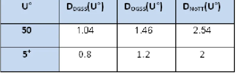
With the increase of uncertainties, the flexibility, as expected, outperformsstatic schedules. Furthermore, looking at Table 2, one can see that performance degradations evolve not very much between U°=5 and U°=50. This tends to prove that, when a certain level of uncertainties is reached, degradation of performances relatively to the lower bound is quite constant (considering the chaotic nature of the measures).

Table 2.Behavior of degradations at extrema of uncertainty degree.

Below, we present the same type of analysis, aggregating the results of all the 15 instances.

Looking carefully at the general evolution of the performances, it is possible to identify three distinct study areas as presented above. However, the boundaries are not always located at U°=0.8 and U°=1.4. There are some slight fluctuations, from U°=0.65 to U°=0.8 for the lowest bound and from U°=1 to U°=1.4 for the highest bound. These fluctuations are in accordance with the instances’ complexity, a complex instance having an intermediate interval higher than a simpler instance. In order to involve all the cases in this generalization, in the following, the areas are defined as:

(1) U°< 0.65, an area with low uncertainties; (2) 0.65< U°< 1.4, called intermediate area;

(3) U°> 1.4, i.e. very low speeds therefore very long transportation time, and very high uncertainties.

d. Area with low uncertainties for all instances

Considering very low uncertainties, NoTT and OGSS are always reaching the Lower Bound (i.e. no degradation). This was expected, as these two schedules are optimized for minimizing the Cmax when no transportation times are taken into account.

DGSS show degradations between 0 and 10%,with an optimal performance in 40% of the instances. These instances correspond to the case where, the decisions, taken during the reactive phase, happen to be optimal if there are taken, by chance, on the critical chain.

When the uncertainties increase, the performances of NoTT and OGSS decrease, as shown with la15. It is interesting to note that given all the instances, the performances of OGSS arevery close toNoTT, sometimes better, more and more frequently as uncertainties increase.

Finally, the chaotic aspect previously shown on the la15 instance is confirmed for DGSS for each instance. On the other side, the stability of NoTT and OGSS is confirmed.

e. Area with high uncertainties for all instances

In that case, the ranking is always the same for all the instances, from the more to the less reactive,

i.e.,DGSS performs the best, then OGSS then NoTT.More precisely, DGSS is better than NoTT from 30

to 60% according to the instances. Yet, OGSS is not so far from DGSS, with a performance lower from 10 to 30%.

6. Discussion

First of all, it is important to explain the chaotic nature of some measures. It can be observed that the more flexible is the schedule (DGSS is the more flexible, then OGSS and then NoTT which has no flexibility), the more chaotic are the measures. It can be explained by the fact that adding flexibility requires that more decisions will be taken in the reactive phase and thus there will be a greater risk of dispersion of the performances. This phenomenon can particularly be observed for instances with more jobs. Once again, the more jobs in an instance, the more decisions are to be taken in the reactive phase, and a greater risk of fluctuations of the performances.

A second point (that is the main contribution of this paper) is that flexibility brings a real added value to absorb uncertainties. We can assess that the more flexible is the schedule, the more robust it appears to absorb uncertainties. It was not so obvious that it seems to be, especially for that kind of uncertainties and that kind of manufacturing system.

For low uncertainties, OGSS is better than NoTT and DGSS. For higher uncertainties DGSS is better than NoTT and OGSS. In all cases, OGSS performs better or at least as well than NoTT. For the record, OGSS is a schedule where the best case quality of the group sequence generated is equal to the

worst case quality without any transfer times. Therefore, it means that the flexibility added without degradation of the worst case quality (without any transfer times) seems very promising. With low uncertainties, the better the quality of the schedule in the worst case, the better the final quality is. This observation is easily explained by the fact that with low uncertainties, it is preferable to stay close to the predictive phase (but with some flexibility), so the better will be the predictive phase, the better will be the reactive phase. And this is confirmed comparing OGSS and DGSS. With low uncertainties, adding flexibility at the price of degrading the worst case quality is not interesting. As a conclusion, group scheduling without degradation of the worst case quality is always better than a static schedule (i.e., without any flexibility). This assertion is relevant with the conclusions of the previous studies on group scheduling from Wu et al. (1999) and Esswein (2003).

Finally, our study shows that group scheduling is particularly efficientto absorb uncertainties caused by the omission of transportation times in the scheduling model.

7. Conclusion

In the field of predictive-reactive scheduling methods, group scheduling is reputed to be robust (in terms of uncertainties absorption) thanks to the flexibility it adds on the sequence of operations. However, this reputation was based on evaluations made on simple theoretical examples.

The aim of this paper is to carry on experimentations on a complex flexible manufacturing system in order to determine whether this flexibility really absorbs uncertainties. The transportation times of the parts between the machines was chosen as the uncertainty to be studied. This choice was lead by the possibility to schedule the FMS with and without taking into account this parameter, which is totally deterministic.

Thus, simulation studies were lead in order to evaluate the relationship between flexibility and ability to absorb uncertainties. The results enable comparing group scheduling of the system with various flexibility levels not taking into account uncertainties, classical scheduling without uncertainties and classical scheduling taking into account the uncertainties. This last schedule is called the lower bound, as it is the best schedule possible.

The results show that the flexibility added in group scheduling is efficient to absorb uncertainties, especially when the level of uncertainties is high. Furthermore, when the level is low, group scheduling shows a good performance, really close to the lower bound. When considering manufacturing systems with a level of uncertainties evolving along time, group scheduling shows good characteristics and performances.

Future works will try to evaluate the performance of group scheduling versus different types of uncertainties (predictive or corrective maintenance for example) or with performance measures related to the due dates such as total tardiness or maximum lateness. As lower bounds are computed off-line in a simplified model which does not take into account the transfer system, the procedure remains the same. Pinot (2008) proposes a branch and bound algorithm which computes the best-case quality for group sequencing for any regular criteria such as the makespan, the total tardiness or the maximum lateness.

Furthermore, a study will be lead on a totally flexible solution, based on product-driven systems paradigm, to evaluate the opportunity of adding more flexibility to group scheduling.

Finally, the group sequence method is one of the only scheduling methods to put into practice human-machine cooperation. The work presented in this paper is also part of a more general thinking on human-machine cooperation in scheduling (Guerin, 2012; Pinot et al., 2009).

8. References

Artigues, C., Billaut, J.-C., Esswein, C., 2005. Maximization of solution flexibility for robust shop scheduling.European Journal of Operational Research. 165(2):314–328.

Bel, G., Cavaillé, J.-B., 2001.Approche simulatoire. In: Lopez, P., Roubellat, F. (Ed), Ordonnancement de la Production, Hermes Publication.

Billaut, J .-C., Moukrim, A., Sanlaville, E., 2004. Introduction. In Billaut, J .-C., Moukrim, A., Sanlaville, E. (Ed), Flexibilité et robustesse en ordonnancement - Traité IC2, Hermes Science, Paris.

Billaut, J.-C., Roubellat, F., 1996. A new method for workshop real-time scheduling.International Journal of Production Research. 34(6), 1555–1579.

Brucker, P.,Jurisch, B.,Sievers, B., 1994. A branch and bound algorithm for the job-shop scheduling problem. Discrete Applied Mathematics. 49(1-3), 107–127.

Buzacott,J.A., Yao, D.D., 1986. Flexible manufacturing systems: A review of analytical models. Management Science, 32 (7), 89–95

Caprihan, R., Kumar, A. and Stecke, K.E.,2006. A fuzzy dispatching strategy fordue-date scheduling of FMSs with information delays.International Journal of FlexibleManufacturing Systems, 18(1), 29-53. Chan, F. T. S., Chan, H. K., Lau, H. C. W., 2002. The State of the Art in Simulation Study on FMS Scheduling: A Comprehensive Survey. International Journal of Advanced Manufacturing Technology, 19, 830–849.

Erschler, J.,Roubellat, F., 1989.An approach for real time scheduling for activities with time and resource constraints. In:Slowinski, R.,Weglarz, J.(Ed), Advances in project scheduling, Elsevier.

Esswein, C., 2003. Un apport de flexibilité séquentielle pour l’ordonnancement robuste. PhD dissertation, Université François Rabelais, Tours.

Goldratt, E.M., 1997. Critical Chain.North River Press.Guérin, C., 2012. Gestion de contraintes et expertise dans les stratégies d’ordonnancement. PhD dissertation, Université de Nantes, France. Lawrence, S., 1984. Resource constrainedprojectscheduling: an experimental investigation of heuristicscheduling techniques (supplement). Technical report, Graduate School of Industrial Administration, Carnegie-Mellon University, Pittsburgh, Pennsylvania.

Pinedo, M. L., 2008. Scheduling: Theory, Algorithms, and Systems.Springer.

Pinot, G., 2008. Coopération homme-machine pour l’ordonnancement sous incertitudes. PhD dissertation, Université de Nantes, France.

Pinot, G., Cardin, O., Mebarki, N., 2007. A study on the group scheduling method in regards with transportation in an industrial FMS. IEEE International Conference on Systems, Man and Cybernetics. Montréal, Québec.

Pinot, G., Mebarki, N., 2008. Best-case lower bounds in a group sequence for the job shop problem. Proceedings of the 17th IFAC World Congress, Seoul, South Korea.

Pinot, G., Mebarki, N., Hoc, J.M., 2008.A New Human-Machine System for Group

Scheduling.Proceedings of International Conference on Industrial Engineering and Systems Management, IESM’2009, Montreal, Canada.

Riezebos, J., Hoc, J.-M., Mebarki, N., Dimopoulos, C., Van Wezel, W., Pinot, G., 2010. Design of scheduling algorithms: Applications. In Fransoo, J.C., Wäfler, T., Wilson, J. (Ed), Behavioral Operations in Planning and Scheduling, Springer, 371-411.

Roubellat, F., Billaut, J.-C., Villaumie, M., 1995. Ordonnancement d’atelier en temps réel : d’ORABAID à ORDO. Revue d’automatique et de productique appliqués. 8(5), 683-713.

Roy, B., 2005. Main sources of inacurratedetermination, uncertainty andimprecision in decisionmodels.Mathematical and Computer Modelling. 12 (10-11), 1245-1254.

Srinoi, P., Shayan, E. and Ghotb, F. (2006).A fuzzy logic modeling of dynamic scheduling in FMS.International Journal of Production Research, 44(11), 2183-2203

Swanson, K., Bresina, J. and Drummond M., 1994.«Just-In-Case Scheduling.» Proceedings of the AAAI

Conference.Seattle.

Thomas, V., 1980. Aide à la décision pour l’ordonnancement d’atelier en temps réel. PhD dissertation, Université Paul Sabatier, Toulouse, France.

Van de Vonder, S., Demeulemeester, E., · Herroelen, W., 2007. A classification of predictive-reactive project scheduling procedures. Journal of Scheduling, 10, 195–207.

Wu, S. D., Byeon, E.-S., Storer, R. H., 1999.A graph-theoretic decomposition of the job shop scheduling problem to achieve scheduling robustness.Operations Research. 47 (1), 113–124.