HAL Id: hal-00668764
https://hal.archives-ouvertes.fr/hal-00668764
Submitted on 10 Feb 2012
HAL is a multi-disciplinary open access
archive for the deposit and dissemination of
sci-entific research documents, whether they are
pub-lished or not. The documents may come from
teaching and research institutions in France or
abroad, or from public or private research centers.
L’archive ouverte pluridisciplinaire HAL, est
destinée au dépôt et à la diffusion de documents
scientifiques de niveau recherche, publiés ou non,
émanant des établissements d’enseignement et de
recherche français ou étrangers, des laboratoires
publics ou privés.
Walking trajectory optimization with rotation of the feet
for a planar bipedal robot with four-bar knees
Arnaud Hamon, Yannick Aoustin
To cite this version:
Arnaud Hamon, Yannick Aoustin. Walking trajectory optimization with rotation of the feet for a
planar bipedal robot with four-bar knees. The ASME 2012 11th Biennial Conference On Engineering
Systems Design And Analysis, Jul 2012, Nantes, France. �hal-00668764�
Proceedings of the ASME 2012 11th Biennial Conference On Engineering Systems Design And Analysis ESDA2012 July 2-4, 2012, Nantes, France
ESDA2012-82580
DRAFT : WALKING TRAJECTORY OPTIMIZATION WITH ROTATION OF THE FEET
FOR A PLANAR BIPEDAL ROBOT WITH FOUR-BAR KNEES.
Arnaud Hamon
Institut de Recherche en Communications et Cybern ´etique de Nantes, L’UNAM, UMR CNRS 6597, CNRS, ´Ecole Centrale de Nantes, Universit´e de Nantes,
1, rue de la No ¨e, BP 92101. 44321 Nantes France
Email: arnaud.hamon@irccyn.ec-nantes.fr
Yannick Aoustin
Institut de Recherche en Communications et Cybern ´etique de Nantes, L’UNAM, UMR CNRS 6597, CNRS, ´
Ecole Centrale de Nantes, Universit ´e de Nantes, 1, rue de la No ¨e, BP 92101. 44321 Nantes
France
Email: yannick.aoustin@irccyn.ec-nantes.fr
ABSTRACT
The design of a knee joint is a key issue in robotics and biomechanics to improve the compatibility between prosthesis and human movements and to improve the bipedal robot perfor-mances. We propose a novel design for the knee joint of a planar bipedal robot, based on a four-bar linkage. The dynamic model of the planar bipedal robot is calculated. We design walking ref-erence trajectories with double support phases, single support s with a flat contact of the foot in the ground and single support phases with rotation of the foot around the toe. During the dou-ble support phase, both feet rotate. This phase is ended by an impact on the ground of the toe of one foot, the other foot taking off. The single support phase is ended by an impact of the swing foot heel, the other foot keeping contact with the ground through its toe. For both gaits, the reference trajectories of the rotational joints are prescribed by polynomial functions in time. A para-metric optimization problem is pres ented for the determination of the parameters corresponding to the optimal cyclic walking gaits. The main contribution of this paper is the design of a dy-namical stable walking gait with double support phases with feet rotation, impacts and single support phases for this novel bipedal robot.
1 Introduction
The researchers in biomechanics have improved a lot the un-derstanding of the human lower limb and especially the knee joint [1] and the ankle joint [2]. Indeed, these two joints have a complex architecture formed by non symmetric surfaces. Their motion is more complex than a revolute joint motion. In the case of the human knee, the joint is formed by different sur-faces, the two non symmetrical femoral condyles and the tibial plateau. This architecture probably appeared in the evolution of many species of animals 320 million years ago. This common ar-chitecture of the knee has not really changed the last 300 million years despite an important diversity of the functional need [3]. The motions of the femur with respect to the tibia are limited due to many ligaments and the patella. In addition to the flexion in the sagittal plane, there is an internal rotation with a displace-ment of the Instantaneous Center of Rotation (ICR) of the knee joint and a posterior translation of the femur on the tibia. These motions are guided by the cruciate ligaments and the articular contacts [4], [1]. These motions cannot be represented by one or two revolute joints. Different studies have confirmed these re-sults by an observation of the motions of the human knee in the 3D space [5].
From these studies, a new kind of prosthetic knee was pro-posed, called polycentric knee. The ICR of the polycentric knees varies with the knee-flexion angle contrary to the axis of single
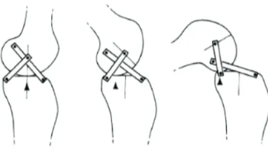
knees. A classical polycentric knee is the four-bar linkage [6], which is used in most prosthetic knees. This architecture forms a closed-loop mechanism, which allows a combined rotation and translation of the knee joint in the sagittal plane without any arti-ficial ligament to keep the rigidity of the mechanism. In 1974, A. Menschik [7] proposed to represent the knee joint by a cross four-bar linkage. This mechanism is the dual solution of the classical four-bar knee but does not have any singularity in the range of motion typically used. As a matter of fact, the kinematic singu-larities of the mechanism may limit its range of motion of, mainly when an important knee flexion is required. The dimensions of the cross four-bar linkage can be chosen by measuring, on a real subject: (i) the length of the anterior and posterior ligaments; (ii) the position of the cross ligament attachments on the tibia and the femur, projected on the sagittal plane in the maximum exten-sion position [8]. As a result, the motions of the mechanical knee joint in the sagittal plane should be similar to the motions of the human knee [4]. In this case, we can reproduce the motion of the knee joint with a posterior displacement of the contact point of the femur on the tibia as shown in Figure 1.
Roboticists have come up with new and better bipedal robots recently. For instance, the HRP-2 [9] and the RABBIT [10], which are able to run, are quite efficient in terms of energy con-sumption. A. Grishin et al. [11] focused on the design of a bipedal robot with telescopic legs. T. Yang et al. [12] used a compliant parallel knee to improve the walking motion. Some authors also dealt with the walking and running gaits using the toe rotation [13], [14], [15]. Our objective is to improve the bipedal robot performance thanks to a new design of the knee joint. Several papers deal with the bipedal robots equipped with complex knees, like G. Gini et al. [16] which used knee joints based on the human knee surfaces. F. Wang et al. [17] developed a bipedal robot with two different joints, namely, a revolute joint and a four-bar linkage. However, the singularities of the common four-bar linkage, i.e., non cross four-bar linkage, usually limit the flexion of the knee. On the contrary, the flexion of the knee joint based on a cross four-bar linkage is usually not too limited with the kinematic singularities. We also proved in [18] that a a knee based on a cross four-bar linkage is better than a knee designed with a revolute joint in terms of energy consumption.
This paper aims to study the performance of a planar bipedal robot equipped with knees based on cross four-bar linkages for complex walking gait composed of double support phase, sin-gle support phase with a flat contact of the foot on the ground and a single support phase with a rotation of the foot around the toe. We also present the dynamic model of a planar bipedal robot whose knees are composed of a cross four-bar linkage. We devel-oped a parametric optimization method to define a set of optimal reference trajectories. We studied the energy consumption of the bipedal robot for different velocities. The main contribution of this paper is the design of a dynamical stable walking gait with double support phases, impacts and single support phases for this
novel bipedal biped. Note that there is a feet rotation around the front heel and the rear toe during the double support phases.
This paper is organized as follows. Section 2 presents the novel planar bipedal robot whose knees are based on four-bar linkages. Section 3 is devoted to the dynamic models. Section 4 deals with the trajectory planning. Section 5 presents numerical results on the walking reference trajectories. Finally, Section 6 presents some conclusions and future works.
FIGURE 1. Representation of the human knee joint composed of a
four-bar linkage. Illustration of the posterior translation of the contact point between the femur and the tibia.
2 Presentation of the bipedal robot with knees com-posed of a four-bar linkage
Let us introduced the bipedal robot, which is depicted in Figure 2. Table 1 gathers the physical data of the biped, which are taken from Hydroid, a humanoid bipedal robot [19].
The dimensions of the four-bar linkage are chosen with re-spect to the human characteristics measured by J. Bradley et al. through radiography in [20].
Masse (kg) Length (m) Inertia (kg.m2) Center of mass (m) foot 0.678 Lp= 0.207 0.002 0.0235 Hp= 0.059 shin 2.188 0.392 0.027 0.223 thigh 5.025 0.392 0.066 0.2234 trunk 24.97 0.403 1.036 0.281 four-bar mb= 0.3 la= AB = 0.029 m knee md= 0.3 lb= BC = 0.030 m lc= CD = 0.015 m ld= AD = 0.025 m
TABLE 1. Physical parameters of the bipedal robot.
q5 q3 q2 q1 q4 qp1 qp2 Γp1 Γp2 Γ2 Γ3
FIGURE 2. Schematic of a planar bipedal robot. Absolute angular
variables and torques.
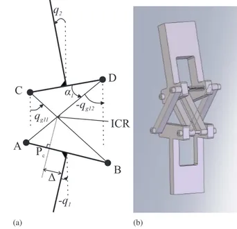
Figures 2; 3(a) and 3(b) depict the bipedal robot under study and its cross four-bar knee linkage. Figure 3(a) represents the cross four-bar knee linkage. The angular variableα1is the
actu-ated variable of the four-bar linkage.
3 Dynamic model
3.1 General dynamic model in double support
The bipedal robot is equipped with two closed-loop knee. Let us introduce the constraint equations solving the dynamic
(a)
q
2q
g11α
1-q
g12ICR
Δ
-q
1P
cA
B
C
D
(b)FIGURE 3. Details of the cross four-bar joint and position of the
In-stantaneous Center of Rotation (ICR)
model [21]. Equations for knee joints 1 and 2 are similar. For a sake of clarity we consider knee joint 1 only. The equations of the closed-loop geometric constraints are defined as follows:
lacos q1−lbsin qg11+ lccos q2+ ldsin qg12= 0
lasin q1+ lbcos qg11−lcsin q2−ldcos qg12= 0
(1)
Their first and second time derivatives are
−la˙q1sin q1−lbq˙g11cos qg11−lc˙q2sin q2+ ld˙qg12cos qg12= 0
laq˙1cos q1−lb˙qg11sin qg11−lc˙q2cos q2+ ld˙qg12sin qg12= 0
(2) and
−la¨q1sin q1−lb¨qg11cos qg11−lc¨q2sin q2+ ld¨qg12cos qg12
−la˙q21cos q1+ lb˙q2g11sin qg11−lc˙q 2
2cos q2−ldq˙2g12sin qg12= 0
la¨q1cos q1−lbq¨g11sin qg11−lc¨q2cos q2+ ld¨qg12sin qg12
−la˙q21sin q1−lb˙q2g11cos qg11+ lc˙q22sin q2+ ld˙q2g12cos qg12= 0.
(3) By using the virtual work principle, these constraints equations can be expressed in the dynamic model by adding the Lagrange multipliers Jt1λ. Here J1is the 2 × 13 Jacobian matrix such as
equations (2) and (3) can be rewritten under the compact forms
and
J1¨x + ˙J1˙x = 0. (5)
and vectorλλλ = fc1 = [ fx1, fy1]t defines the two Lagrange
multi-pliers vector associated to the constraint of the closed structure. These multipliers represent the exerted forces on point A of the knee joint 1 (Figure 3(a)). We apply the same principle for the knee joint 2 to obtain the dynamic model of the bipedal robot with the cross four-bar knees:
A(x)¨x + h(x, ˙x) = !DΓJt1Jt2 "#ΓΓΓmmm fc $ + Jtr1r1 + J t r2r2 (6)
with the constraint equations:
Jri¨x + ˙Jri˙x = 0 for i = 1 to 2 #J1 J2 $ ¨x + #˙J 1 ˙J2 $ ˙x = 0 (7) ΓΓΓmmm= [Γp1, Γp2, Γ1, Γ2, Γ3, Γ4]
tis the vector of the applied joint
torques and fc= [ftc1, f t
c2]
t. The generalized vector x is such as
x = [qp1, qp2, q1, · · · , q5, qg11, qg12, qg21, qg22, xh, yh] t
where xhand yhare the hip coordinates. Jr1 and Jr2 are the 3 ×
13 jacobian matrix of the constraint equations in position and orientation for the two feet, respectively. A(x) is the 13 × 13 symmetric positive definite inertia matrix, h(x, ˙x) is the 13 × 1 vector, which groups the centrifugal, Coriolis effects, and the gravity forces. DΓis a 13 × 6 matrix composed of the 0 and ±1
given by the principle of virtual works [22].
This dynamic model (6) with constraints (7) is valid in sin-gle support and double support phases. During a sinsin-gle support phase the ground reaction force is zero on the swing foot.
3.2 Reduced model in single support
The aim is to propose a dynamic model with an implicit li-aison of the stance foot with the ground to calculate the torques during the optimization process, with the knowledge of the ref-erence trajectories for the generalized coordinates. This reduced dynamic model is only valid if the stance foot does not take off and there is no sliding during the swing phase.
Then, during the single support phase, the stance foot is as-sumed to remain in flat contact on the ground, i.e., there is no sliding motion, no take-off, no rotation (qp1= 0). We can use a
new generalized vector q = [qp2, q1, · · · , q5, qg11, qg12, qg21, qg22]t.
The reduced dynamic model does not depend on the ground re-action force, which is applied in the stance flat-foot. The dy-namic model in single support phase for the biped equipped with the four-bar knees is given by the simplification of the dynamic model (6) and (7):
A(q) ¨q + h(q, ˙q) =!DΓJt1Jt2"#ΓΓΓmmm
fc
$
. (8)
with the constraints equation, #J1 J2 $ ¨q + #˙J 1 ˙J2 $ ˙q = 0. (9)
Here vector fcis such as fc= [ftc1, f t c2] t.
x
y
Hp lp l ZMP Lpz
Gf spx spy r P OFIGURE 4. Details of the foot.
To define the constraints about the ground reaction, the no take-off of the stance flat-foot during the optimization process, we recall the calculation of position of the Zero Momentum Point. The center of mass Gf of the foot is assumed located on
the vertical axis, crossing the joint ankle, Figure 4. The resultant force R of the ground reaction can be calculated by applying the second Newton law at the center of mass of the biped:
mγγγ= r + mg, (10)
where m is the global mass of the biped,γγγ= [ ¨xg, ¨yg]tare the
hor-izontal and vertical components of the acceleration for its center of mass in the world frame. g = [0, −g]tis the vector of the ac-celeration of the gravity. This equation allows directly to get r
during the single support. Assuming the center of mass Gf of
the foot has for coordinates (spx, spy), see Figure 4. Let mf be
the mass of the foot. The application point P of this resultant force r = [rx, ry, rz]t of the ground reaction, where the moment
m = [mx, my, mz]t has its components, which are null following
axes x and z, mx = mz = 0, is called the Zero Moment Point.
One necessary and sufficient condition for the foot to keep the flat contact is, that P belongs to the convex hull of the support-ing area (Vukobratovic [23]). In this case the ZMP is merged with the center of pressure. Let fOand mObe the force and the
moment exerted by the mechanism above the ankle, defined by point O, of the supporting foot. Let us state the static equilibrium in rotation for the supporting foot:
mO+ OO × FO+ OGf×mfg + OP × r + m = 0, (11)
where OP, OGf and OO are radius vectors from the origin of
the coordinate system O. For the planar biped the coordinate of the ZMP can be obtained through the calculation of the global equilibrium of the bipedal robot around axis z, which gives:
lZMP=Γp1+ spxmfg − Hprx
ry , (12)
where Γp1 is the applied torque on the ankle.
To calculate the applied joint torques, which are used to ob-tain the energy consumption of each bipedal robot during the op-timization process, we use the dynamic model (8).
We assume the friction effects due to the cross four-bar mechanism are negligible with respect to those in the gearbox of the actuators. Then only the performances of actuators are considered to compare the energy consumption for the biped equipped with both types of knee joints successively. No fric-tion terms are included in the model.
3.3 Impact model
During the biped’s gait, impacts occur, when the sole, the heel or the toe of the swing foot swing touches the ground. Let
T be the instant of an impact. We assume that the impact is
ab-solutely inelastic and that the foot does not slip. Given these conditions, the ground reactions at the instant of an impact can be considered as impulsive forces and defined by Dirac delta-functions rj= ijδ(t − T ) ( j = 1, 2). Here ij = [ijx, ijy]t is the
magnitudes vector of the impulsive reaction in foot j (see [24]). Impact equations can be obtained through integration of the ma-trix motion equation (6) for the infinitesimal time from T− to
T+. The torques provided by the actuators in the joints, Coriolis and gravity forces have finite values. Thus they do not influence the impact. Consequently the impact equations can be written in
the following matrix form:
A(x(T ))(˙x+−˙x−) =!Jt
1Jt2" ifc+ Jtr1i1+ J t
r2i2 (13)
Here x(T ) denotes the configuration of the biped at instant
t = T , (this configuration does not change at the instant of the
impact), ˙x−and ˙x+are respectively the velocity vectors just
be-fore and just after an inelastic impact. To take into account of the closed-loop of the four-bar knee linkage we have to complete (13) with:
#J1 J2
$
˙x+= 0 (14)
The velocity of the contact part of the stance foot ( j = 1) before an impact is null.
Jr1˙x
−= 0 (15)
The swing foot ( j = 2) after the impact becomes a stance foot. Therefore, the velocity of its contact part with the ground be-comes zero after the impact,
Jr2˙x
+= 0 (16)
Generally speaking, two results are possible after the impact, if we assume that there is no slipping of the stance feet. The stance foot lifts off the ground or both feet remain on the ground. In the first case, the vertical component of the velocity of the taking-off foot just after the impact must be directed upwards. Also there is no interaction (no friction, no sticking) between the taking-off foot and the ground. The ground reaction in this taking-off leg tip must be null. In the second case, the stance foot velocity has to be zero just after the impact. The ground produces impulsive reactions (generally, ij $= 0, j = 1, 2) and the vertical
compo-nents of the impulsive ground reactions in both feet are directed upwards. For the second case, the passive impact equation (13) must be completed by one matrix equations.
Jr1˙x
+= 0 (17)
In general, the result of an impact depends on two factors: the biped’s configuration at the instant of an impact and the direc-tion of the swing foot velocity just before impact [24]. After an impact for a biped, there are two possible phases: a single sup-port or a finite time double supsup-port.
The resolution of the system composed (13), (14), (16) and eventually (17) gives the velocity vector ˙x+ just after the im-pact, the impulsive reaction forces i1, i2and the impulsive forces
ifc= [itfc1, i
t
fc2]
trelatively to the velocity vector ˙x−just before the
impact.
To calculate the position of the ZMP at the impact with flat-foot, we have to take into account of the impulsive ground re-action in the global equilibrium of the stance foot and the result is:
lZMP= −
Hpijx
ijy . (18)
4 Gait optimization for the cyclic walking 4.1 Principle
The biped is driven by six torques, and its configuration is given by vector q of generalized coordinates. To transform the optimization problem into a finite dimension problem, the joint motion is described as a parametric function. We choose, for each phase, a cubic spline function of time.
To insure continuity between two successive phases, the po-sition and velocity of the biped at the beginning and at the end of each phase must be taken into account by the parameters of the cubic spline functions.
To design a cyclic walking gait, the behavior of the actuated joint variables are prescribed using cubic spline functions. The set of parameters are used to calculate these cubic spline func-tions, taking into account the properties of continuity between each step. From the final state of a step to the initial state of the following step, there is an exchange of the number of the joints, since the legs swap their roles, we have:
qp1i= qp2 f, q1i= q4 f, q2i= q3 f and q5i= q5 f. (19)
Values for these parameters are calculated by minimizing a criterion based on the energy consumption. Physical conditions of contact between the feet and the ground and limits on the ac-tuators define non-linear constraints of this optimization process.
4.2 Studied gait
The studied gait is composed of three different phases : a double support phase with rotation of both feet, a single support phase with a flat contact foot on the ground and single support phase with rotation of the foot around the toe. The double sup-port phase ends by the flat contact of the forward foot on the ground that occurred an impact. The single support phase with rotation of the foot ends by the contact on the ground of the swing foot on the heel that also occurred an impact.
During the single support phase with rotation of the foot, the biped is under actuated. The time evolution of the biped cannot be prescribed directly. To determine the evolution of the biped during this phase, it is possible to parametrise the evolution of
each joint i, (i = 1, · · ·, 7) according to a configuration param-eter that depends on the biped dynamic [19]. The evolution of each joint is given by a fourth order polynomial function of the configuration parameter s: qi(s) = a0i+ a1is + a2is 2+ a 3is 3+ a 4is 4 ∂qi(s) ∂s = a1i+ 2 a2is + 3 a3is2+ 4 a4is3 ∂2qi(s) ∂s2 = 2 a2i+ 6 a3is + 12 a4is 2 (20)
The evolution of s, ˙s et ¨s is obtained by the computation of the angular momentum around the point of rotation. The angu-lar momentum is a linear function with respect to the velocity components. Then tacking into account of (20) we can write the angular momentum as a function of s and ˙s such that:
σO(s, ˙s)! I(s) ˙s (21)
Moreover, the dynamic momentum is given by : ˙
σO(s) = −m g xg(s) (22)
So, we have :
σO(s, ˙s) dσO(s) = −m g xg(s) I(s) ds (23)
where m is the mass of the robot, g is gravity acceleration and xg
is the horizontal coordinate of the biped center of mass. By integration from 0 to s : 1 2 ! σ02(s, ˙s) −σ02(0, ˙s0)" = − ) s 0 m g xg(ξ) I(ξ) dξ (24) which gives : 1 2I 2(0) ˙s2 0= 1 2I 2(s) ˙s2+ V (s) (25) with : V (s) = m g ) s 0 I(ξ)xg(ξ) dξ (26)
So, we can determine the evolution of ˙s in function of its initial value for s = 0 with :
˙s = *
I2(0) ˙s2
0−2 V (s)
From equations (21) and (22), we obtain ¨s :
¨s =−m g xg(s) − I(s)
2 ˙s2
I(s) (28)
4.3 Parametric optimization problem
By parameterizing the joint motion in terms of cubic spline functions, the optimization problem is reduced to a constrained parameter optimization problem of the form:
Minimize CW (P)
subject to gj (P) ≤ 0 for j = 1, 2, ...l (29)
where P is the set of optimization variables. CW(P) is the
crite-rion to minimize with l inequality constraints gj(P) ≤ 0 to
sat-isfy. The criterion and constraints are given in the following sec-tions.
We used the SQP method (Sequential Quadratic Program-ming) [25], [26] with the fmincon function of Matlab!R to solve this problem.
4.3.1 The criterion Many criteria can be used to pro-duce an optimal trajectory. A sthenic criterion is chosen to obtain optimal trajectories: CW =1 d ) T 0 6
∑
i=1 ΓtmiΓmidt, (30)where T is the step duration and ˙θi is the joint velocities
asso-ciated to torque Γmi. During an optimization process the step
length d is an optimization variable and the walking speed v is fixed, such as the step duration is directly given through the rela-tion T = d/v.
However, the duration of the single support phase with rota-tion of the foot cannot be fixed on the optimizarota-tion process, but the integration of the function ˙s gives the duration of this phase. To set the walking velocities, we add to the optimization crite-rion the error between the the desired velocities and the obtained velocities with a penalty factor :
C = CW+ 108(vd−v) (31)
where vdis the desired velocity and v is the velocity deduce from
the step duration.
The resulting optimal control is continuous and cancels the risks of a jerky functioning [27]. This smoothness property also guarantees a better numerical efficiency for the algorithm used for the optimization problem-solving.
4.3.2 Optimization parameters To describe the
evo-lution of the articular variable q, we use polynomial functions. During the double support phase the configuration of the biped is described by 7 variables and we use third order polynomial func-tions to prescribe their trajectories. During the single support phase the configuration of the biped is described by 6 variables and we use also third order polynomial function. Finally, for the single support phase with rotation of the foot around the toe, the configuration of the biped is given by 7 variables and we use fourth order polynomial function of the configuration parameter
s to describe the biped trajectory.
In consequence, the 3 different functions used to describe the evolution of an articular variable allow to prescribe the initial and final position and velocity for each phase of a step and a in-termediate position during the single support phase with rotation of the foot.
The objective of the optimization algorithm is to determine the different initial and final position and velocities and the in-termediate position to minimize the optimization criteria and to respect the constraints. To reduced the complexity of this prob-lem and to develop cyclic trajectories we take into account the continuity between the different phases and between the differ-ent step. So, finally the number of optimization variables needed to describe a trajectory is given on the table 2.
4.3.3 The constraints Two types of constraints are
used to obtain a realistic gait.
The necessary constraints, which ensure a valid walking gait. The first constraint ensures the supporting leg tip does not take off or slide on the ground. So, the ground reaction force is inside a friction cone, defined with the coefficient of friction f :
+ max(− f riy−rix) ≤ 0
max(− f riy+ rix) ≤ 0 (32)
j = 1 or 2. rx and ry are the normal and tangential
com-ponent of the reaction force. Moreover, we can introduce a constraint on the ground reaction at the impact:
+ (− f i1y−i1x) ≤ 0
(− f i2y+ i2x) ≤ 0 (33)
To ensure the non rotation of the supporting foot we in-troduce a constraint on the ZMP during the single support phase and at the instant of the impact:
Phase Variables Parameters Double support q(0) q(Tds) ˙q(0) ˙q(Tds) R2x Tds 7 7 7 7 3 1 5 5 3 1 Single support q(Tds) q(Tss) ˙q(Tds) ˙q(Tss) Tss 6 6 6 6 1 6 6 1 Single support with rota-tion q(Tss) q(T ) q((T + Tss)/2) ˙q(Tss) ˙q(T ) ˙s0 7 7 7 7 7 1 5 7 7 1 Total 93 47
TABLE 2. Table of the optimization parameters. Tssis the instant of
the end of the single support phase. Tdsis the instant of the end of the
double support phase. T is the step duration.
Here Lp is the length of the foot and lpis the distance
be-tween the heel and the ankle along the horizontal axis, see Figure 4.
Just after the impact, the velocity of the taking-off foot should be directed upward. In consequence, the positivity of the vertical component of the velocities for the heel and the toes is added to the set of constraints.
The last constraint allows to ensure the non penetration of the swinging foot in the ground.
The unnecessary constraints, which ensure a technological realistic gait. We introduced mechanical stops on the joint variables. Moreover, we limited the torques with a con-straint, which sets a template of the maximum torque of the motor relatively to the velocity [10].
FIGURE 5. Stick diagram of a walking trajectory for a walking
ve-locity of 2.2 Km/h.
5 Results
In this part, we use the parametric optimization method, pre-sented previously, to produce a set of optimal reference walking trajectories for the biped with four-bar knees.
The figure 5 present a walking trajectory obtains for a walk-ing velocity of 2.2 Km/h. We can see the three different phases. The value of the optimization criterion for this gait is CΓ =
1942 N.m.s−1.
On figure 6, we can see the evolution of the energy criterion according to the walking velocity. We can note a minimum en-ergy consumption for a velocity of 2.35 Km/h. Moreover, we can see the energy criterion increases quickly when we reduce the walking velocities. This result can be explained by the diffi-culty to produce walking trajectories with rotation of the foot for low speed. A walking trajectory without rotation would probably be more effective.
The figure 7 gives the orientation of the support foot at the end of the step in function of the walking velocities. This figure shows the rotation of the support foot during the single support phase increased when you increase the walking velocity.
6 Conclusions
As a conclusion of this work, we present a planar bipedal robot equipped of four-bar linkages for the knee joints. We present the dynamic model of this robot and a parametric op-timization method to produce optimal walking trajectories com-posed of double support phase, single support phase with a flat contact of the foot on the ground and a single support phase with a rotation of the support foot around the toe. Models of
impul-1.4 1.6 1.8 2 2.2 2.4 2.6 2.8 3 0 1000 2000 3000 4000 5000 6000 7000 v (Km/h) Cw (N 2.m .s )
FIGURE 6. Evolution of the energie criterion CW according to the
walking velocities. Quadratic fitting of the evolution of the optimization criterion (solid line).
1.4 1.6 1.8 2 2.2 2.4 2.6 2.8 3 −20 −18 −16 −14 −12 −10 −8 −6 −4 −2 0 v (Km/h) qp 1 (T )
FIGURE 7. Evolution of the orientation of the support foot at the end
of the step according to the walking velocities.
sive impacts are presented and used during the transition of the different phases. The numerical results have shown this original biped can performed human like walking with a rotation of the foot without actuation of the toe during the single support phase. In perspective of this work an extension in 3D can be done. Moreover, a comparison of the walking trajectories obtained for this biped with human movement can proved the higher
compat-ibility of this biped than a classical biped equipped of revolute knee joints.
ACKNOWLEDGMENT
This work is supported by ANR grants for the R2A2.
REFERENCES
[1] Wilson, D. R., Feikes, J. D., and O’Connor, J., 1998. “Lig-aments and articular contact guide passive knee flexion”.
Journal of Biomechanics, 31, pp. 1127–1136.
[2] Leardini, A., O’Connor, J., Catani, F., and Giannini, S., 1999. “A geometric model of the human ankle joint”.
Jour-nal of Biomechanics, 32(6), pp. 585 – 591.
[3] Dye, S., 1987. “An evolutionary perspective of the knee”.
The Journal of Bone and Joint Surgery, 69(7), pp. 976–983.
[4] Fuss, F. K., 1989. “Anatomy of the cruciate ligaments and their function in extension and flexion of the human knee joint”. American Journal of Anatomy, 184(2), pp. 165– 176.
[5] Landjerit, B., and Bisserie, M., 1992. “Cin´ematique spa-tiale de l’articulation f´emoro-tibiale du genou humain : car-act´erisation exp´erimentale et implications chirurgicales”.
Acta Orthopaedica Belgica, 58(2), pp. 147–158.
[6] Gard, S. A., Childress, D. S., and Uellendahl, J. E., 1996. “The influence of four-bar linkage knees on prosthetic swing-phase floor clearance”. Journal of Prosthetics and
Orthotics, 8(2), pp. 34–40.
[7] Menschik, A., 1974. “Mechanics of the knee-joint. part i.”.
Z Orthop Ihre Grendgeb, 112(3), pp. 481–495.
[8] Feikes, J. D., O’Connor, J. J., and Zavatsky, A. B., 2003. “A constraint-based approach to modelling the mobility of the human knee joint”. Journal of Biomechanics, 36(1), pp. 125 – 129.
[9] Kaneko, K., Kanehiro, F., Kajita, S., Hirukawa, H., Kawasaki, T., Hirita, M., Akachi, K., and Isozumi, T., 2004. “Humanoid robot hrp-2”. In Proceedings of the In-ternational Conference on Robotics and Automation 2004, pp. 1083–1090.
[10] Chevallereau, C., Abba, G., Aoustin, Y., Plestan, F., West-ervelt, E., Canuddas-de Wit, C., and Grizzle, J., 2003. “Rabbit: a testbed for advanced control theory”. IEEE
Con-trol Systems Magazine, 23(5), pp. 57–79.
[11] Grishin, A., Formal’sky, A., Lensky, A., and Zhitomirsky, S., 1994. “Dynamic walking of a vehicle with two tele-scopic legs controlled by two drives”. The International
Journal of Robotics Research, 13(2), pp. 137–147.
[12] Yang, T., Westervelt, E., Schmideler, J., and Bockbrader, R., 2008. “Design and control of a planar bipedal robot ernie with parallel knee compliance”. Autonomous robots,
[13] Kajita, S., Kaneko, K., Morisawa, M., Nakaoka, S., and Hirukawa, H., 2007. “Zmp-based biped running enhanced by toe springs”. In 2007 IEEE International Conference on Robotics and Automation, pp. 3963–3969.
[14] Tajima, R., Honda, D., and Suga, K., 2009. “Fast running experiments involving a humanoid robot”. In 2009 IEEE Conference on Robotics and Automation, pp. 1571–1576. [15] Tlalolini Romero, D., Aoustin, Y., and Chevallereau, C.,
2009. “Design of a walking cyclic gait with single support phases and impacts for the locomotor system of a thirteen-link 3d biped using the parametric optimization”.
Multi-body System Dynamics, 23(1), pp. 33–56.
[16] Gini, G., Scarfogliero, U., and Folgheraiter, M., 2007. “Human-oriented biped robot design : insights into the de-velopment of a truly antropomophic leg”. In IEEE Interna-tional Conference on Robotics and Automation, pp. 2910– 2915.
[17] Wang, F., Wu, C., Zhang, Y., and Xu, X., 2007. “Design and implementation of coordinated control strategy for biped robot with heterogeneous legs”. In IEEE International Con-ference on Mechatronics and Automation, pp. 1559–1564. [18] Hamon, A., and Aoustin, Y., 2010. “Cross four-bar linkage for the knees of a planar bipedal robot”. In 2010 IEEE-RAS International Conference on Humanoid Robots.
[19] Tlalolini Romero, D., Chevallereau, C., and Aoustin, Y., 2009. “Comparison of different gaits with rotation of the feet for a planar biped”. Robotics and Autonomous Systems,
57(4), Avril, pp. 371–383.
[20] Bradley, J., FitzPatrick, D., Daniel, D., Shercliff, T., and O’Connor, J., 1988. “Orientation of the cruciate ligament in the sagittal plane”. The Journal of bone and joint surgery,
70-B, pp. 94–99.
[21] Khalil, W., and Dombre, E., 2002. Modeling, identification
and control of robots. Hermes Sciences Europe.
[22] Appell, P., 1931. Dynamique des Syst`emes - M´ecanique
Analytique. Gauthiers-Villars.
[23] Vukobratovic, M., and Stepanenko, J., 1972. “On the sta-bility of anthropomorphic systems”. Mathematical
Bio-sciences, 15(1), pp. 1–37.
[24] Formal’skii, A., 1982. Locomotion of Anthropomorphic
Mechanisms. [In Russian], Nauka, Moscow, Russia.
[25] Gill, P., Murray, W., and Wright, M., 1981. Practical
opti-mization. Academic Press, London.
[26] Powell, M., 1977. Variable metric methods for constrained
optimization. Lecture Notes in Mathematics. Springer Berlin / Heidelberg, pp. 62–72.
[27] Chevallereau, C., Bessonnet, G., Abba, G., and Aoustin, Y., 2009. Bipedal Robots. ISTE Wiley.