Fuel cells static and dynamic characterizations as tools for the estimation of their ageing time

HAL Id: hal-00985761

https://hal.archives-ouvertes.fr/hal-00985761

HAL is a multi-disciplinary open access archive for the deposit and dissemination of sci-entific research documents, whether they are pub-lished or not. The documents may come from teaching and research institutions in France or abroad, or from public or private research centers.

L’archive ouverte pluridisciplinaire HAL, est destinée au dépôt et à la diffusion de documents scientifiques de niveau recherche, publiés ou non, émanant des établissements d’enseignement et de recherche français ou étrangers, des laboratoires publics ou privés.

Fuel cells static and dynamic characterizations as tools

for the estimation of their ageing time

Raissa Onanena, Latifa Oukhellou, Denis Candusso, Fabien Harel, Daniel

Hissel, Patrice Aknin

To cite this version:

Raissa Onanena, Latifa Oukhellou, Denis Candusso, Fabien Harel, Daniel Hissel, et al.. Fuel cells static and dynamic characterizations as tools for the estimation of their ageing time. International Journal of Hydrogen Energy, Elsevier, 2011, 36 (2), pp. 1730-1739. �10.1016/j.ijhydene.2010.10.064�. �hal-00985761�

• R. Onanena, L. Oukhellou, D. Candusso, F. Harel, D. Hissel, P. Aknin. Fuel cells static and dynamic characterizations as tools for the estimation of their ageing time. Accepté dans International Journal of Hydrogen Energy le 22/10/2010. Ed. Elsevier.

Fuel cells static and dynamic characterizations as tools for the estimation of

their ageing time

R. Onanena a,b,c, L. Oukhellou c,d,*, D. Candusso a,c,*, F. Harel a,c, D. Hissel a,b, P. Aknin c

a

FC LAB, Techn’Hom, rue Thierry Mieg, 90010 Belfort Cedex, France

b

FEMTO-ST (UMR CNRS 6174), ENISYS Department, University of Franche-Comté, France

c

INRETS, "Le Descartes 2", 2 rue de la butte verte, 93166 Noisy-le-Grand Cedex, France

d

CERTES Université Paris 12, 61 avenue du Gal. De Gaulle, 94100 Créteil, France

* Corresponding author.

Tel.: +33 (0)1 45 92 56 58; Fax: +33 (0)1 45 92 55 01; E-mail addresses:

raissa.onanena@inrets.fr (Raïssa Onanena), latifa.oukhellou@inrets.fr (Latifa Oukhellou), denis.candusso@inrets.fr (Denis Candusso), fabien.harel@inrets.fr (Fabien Harel), patrice.aknin@inrets.fr (Patrice Aknin), daniel.hissel@univ-fcomte.fr (Daniel Hissel).

Keywords:

Abstract

This paper deals with a pattern-recognition-based diagnosis approach, which aim is to estimate the Fuel Cell (FC) operating time, and consequently its remaining duration life. With the method proposed, both static and dynamic information extracted from the stack (i.e. polarization curve records and Electrochemical Impedance Spectroscopy (EIS) measurements) can be used. The complete diagnosis method consists of several steps. First, features are extracted from EIS measurements and polarization curves independently. This enables us to simplify the extracted information without losing relevant information, and to remove noise. For the polarization curves, an empiric model is exploited to ensure the feature extraction. For the impedance spectra, both expert knowledge and parametric modeling are used to extract features. In particular, a latent regression model is used to split automatically the imaginary part of the spectra into several segments that are approximated by polynomials. The next step of the method consists in selecting the most relevant features from the whole set of extracted features. This helps us to estimate the operating time, while adjusting the complexity of the model. The final step of the approach is a linear regression that uses the selected subset of features to estimate the FC operating time. The performances of the proposed approach are evaluated on a dataset made up of EIS measurements and polarization curves extracted from two FC lifetime tests. A mean error of about 2 hours over a global operating duration of 1000 hours can be obtained. Moreover, the portability of the method is shown by considering another FC ageing test conducted on a different FC stack type.

1. Introduction

PEM Fuel Cells (FC) are electrochemical systems that convert directly hydrogen energy into electrical energy with high efficiency, and no CO2 emission. That is why those systems appear

as promising technology solutions, especially for transports. However, FCs still suffer from a low reliability and a short lifetime, which make them difficult to meet today's requirements. Indeed, a minimal lifetime of 5000 hours is required for stacks dedicated to vehicular applications [1,2]. It is therefore important to accurately predict FC state-of-health and remaining duration time. For that purpose, it is necessary to develop diagnosis schemes that can evaluate FC state-of-health adequately, especially for maintenance purposes. Therefore, it is important to establish a link between the FC degradation phenomenon and the FC physical characterizations that can be employed throughout ageing time to estimate the FC lifetime, and consequently the remaining duration life during operations.

Previous studies have been conducted to evaluate FC stack performances through the time evolution of various parameters [3-5]; others have been done to estimate the FC operating time (respectively lifetime) by using Electrochemical Impedance Spectroscopy (EIS) measurements [6].

In previous studies, we have used a pattern-recognition-based approach to estimate the FC operating time, using EIS measurements (dynamic characterizations) only [7,8]. With this work, we obtained an estimation of the operating time with a mean square error on the test set of 95 hours over a total duration of 1000 hours. It seemed then interesting to investigate the possible improvement of the results, when using both dynamic and static characterizations. This paper focuses on this issue. Therefore, in the following, the same pattern-recognition-based approach is exploited on the same FCs that were used in [8], and both EIS measurements and polarization curves are considered (first separately, then combined) for the estimation of the operating time. In addition, the portability of the method is shown by considering another FC ageing test conducted on a different FC stack type.

The paper is organized as follows. In Section 2, the principle of the pattern-recognition-based approach will be presented. In Section 3, the two FC characterizations are detailed, especially their relevance regarding the estimation of the FC operating time. Feature extraction and selection methods are presented in Sections 4 and 5. The test procedure for the operating time estimation is given in Section 6. The performances of the proposed approach obtained on real datasets are summarized in Section 7.

2. Principle of the pattern-recognition-based approach

A pattern-recognition-based diagnosis aiming to estimate the FC operating time from both EIS measurements and polarization curves is here presented. The intrinsic aim is to exploit both static and dynamic information that are extracted from the stack to estimate the FC operating time, and consequently its remaining duration life.

The complete diagnosis tool, presented in Fig. 1 consists of several steps. First, FC undergoes a characterization process: EIS measurements and polarization curves are performed. Then the second step is a feature extraction that consists in generating features from polarization curves and EIS measurement independently. This step aims at first summarizing efficiently the measurements without losing relevant information, and then at removing noise. For the polarization curves, two empiric models are employed for feature extraction. As for impedance spectra, various methods based on expert knowledge can be used to extract features [9,10]. Particular points (or hyperparameters) are first empirically extracted and tested. Then, two parametric modeling are performed on the real and the imaginary parts of the spectrum. In particular, a latent regression model is exploited to split automatically the imaginary part of the spectrum into several segments that correspond to different FC physical behaviors. The third step is feature selection. This step enables to select the most relevant features from the whole set of extracted features to estimate the operating time, while adjusting the complexity of the chosen model. Indeed, a tradeoff has to be made between complexity (i.e. the number of selected features) and accuracy in order to avoid the well-known phenomenon of overfitting [11,12]. While an overly complex model could pass exactly through all the experimental points, it could also lead to a poor representation of the real phenomenon. However, the reverse situation of an overly simple model (less complexity) could also lead to a poor representation of the phenomenon. Furthermore, dimensionality reduction is also essential to avoid overfitting when the available training data set is small as it is in our case. The final step of this approach is a linear regression that uses the selected subset of features to estimate the FC operating time. In fact, this operating time is an equivalent period that corresponds to the elapsed time during which an identical FC operates under nominal conditions.

3. Fuel cell characterization

Durability tests were performed on two identical small power PEMFCs (three-cell stacks of about 100 W) during 1000 hours. These stacks have been assembled with graphite gas distributive plates, commercial membranes (Gore MESGA Primea MEA Series 5510; active cell area of 100 cm2) and Gas Diffusion Layers (GDLs) [1,2]. The first stack (FC1) was operated in nominal and stationary conditions. The load current was constant and equal to 50 A. In the second test, the fuel cell (FC2) was operated under dynamical load current based on a real transportation mission profile (maximum current of 70 A was reached for an average of 12.5 A). For both stacks, the set of anode/cathode stoichiometry rates was fixed to 2/5. Details on the test conditions and kind of current solicitation can be found in [1,2], as well as the complete characterization test results. During these ageing tests, the stacks were characterized regularly (twice per week) through polarization curves and impedance spectra.

3.1. Polarization curves

The polarization curve gives information about the static behavior of the FC. It is a powerful tool for various applications such as FC characterization, ageing studies, or diagnosis. In order to realize a polarization curve, one has to make sure that the operating conditions (temperatures, pressures, humidities…) are stable. Therefore, before every series of characterization, the FCs were operated under the same operating point for 30 minutes [1,2].

In general, depending on the current density interval, polarization curves can reveal three different internal behaviors of the FC [13,14] (see Fig. 2). In low current densities, the curves illustrate charge transfer kinetics; in medium current densities, the slope and form of the polarization curves are highly influenced by ohmic resistance; and finally in high current densities, the influence of the mass transfer is highlighted.

As it can be seen in Fig. 2, both the form and the slope of polarization curves vary through time, during the ageing experiments. This leads us to believe that a parameterization of polarization curves can be helpful to provide suitable indicators relating to the ageing phenomenon in FCs.

Fig. 2 - Presentation of the three parts of the polarization curve (left) and evolution of the polarization curves for FC1 stack from the initial state (Time : 0 h) to the final state (Time : 995

h) (right).

3.2. Electrochemical Impedance Spectrum

Unlike the polarization curve, Electrochemical Impedance Spectroscopy (EIS) enables us to obtain relevant information about the dynamical behavior of the FCs during an ageing process [16-18]. EIS allows the characterization of dynamic processes occurring at different timescales

in the system. Considering this technique, the FC is placed on a static operating point and then additional small amplitude solicitation signals are applied. In our case, both stacks were placed under the operating point of 35A, and a small sinusoidal alternating part (with amplitude of 1 A and frequency range from 10 mHz to 30 kHz) was applied around it. Each recorded impedance spectrum was a series of impedance measurements at 45 discrete frequency points.

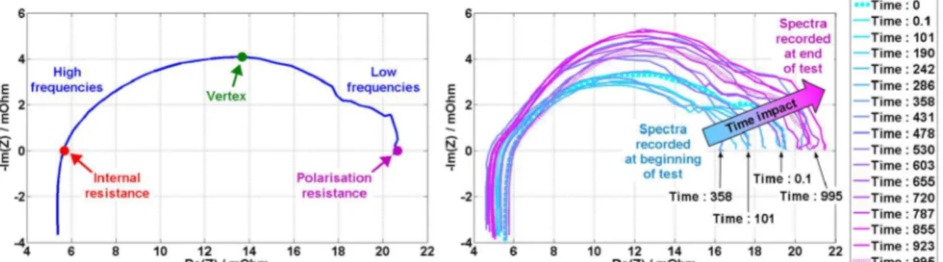
The different ageing test conditions applied on both stacks have led to different EIS results for each FC [1,2]. As an example, the impedance plots measured during the ageing test conducted on FC1 stack are presented in Fig. 3. It can be observed that the FC impedance can be divided into three parts, each part corresponding to a distinct dynamic behavior:

− a first capacitive arc (f < 130 Hz) due to mass and water transports,

− a second capacitive arc (130 Hz < f < 4 kHz) due to the charge (electrons and protons) transfer processes,

− an inductive part which is present in high frequencies (4 kHz < f) due to connections (internal and external ones).

The delimiting frequency values presented above are approximate values, and they depend on the FC and its ageing state. Our goal is to use these characteristics, especially their evolution to estimate the FC operating time. Indeed, they seem to be good indicators of the ageing phenomenon in FCs. More details on physical processes behind these intervals can be found in [1,2].

Fig. 3 - Presentation of hyperparameters in the impedance spectrum (left) and evolution of the impedance spectra for FC1 stack from the initial state (Time : 0 h) to the final state (Time: 995

h) (right).

4. Feature extraction

The goal of this processing phase is to generate automatically a subset of features that will represent the data. The underlying motivation is that the data can be represented in a subspace whose intrinsic dimensionality is lower than the one of the original data space [12].

4.1. Feature extraction on the polarization curves

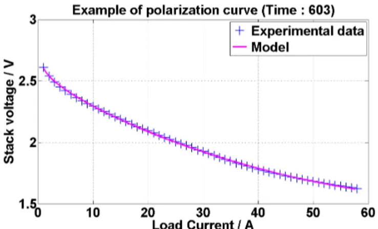
Feature extraction on a polarization curve consists in approximating it by external model and using afterwards the model parameters as features. Previous studies on FCs have underlined many empiric models of polarization curves [18]. The following model is investigated here:

Moreover, the experimental results have shown that the open circuit voltage (noted U0) is

linked to the ageing phenomenon (see Fig.2). Therefore, the number of extracted parameters for the polarization is five (U0, α1, α2, α3, α4). Figure 4 presents the behavior of the model obtained

on a polarization curve modeling.

Fig. 4 - Example of an approximation of a polarization curve.

4.2. Feature extraction on the EIS

For the impedance spectra, two different methods were considered. The first one, based on expert knowledge, consists in the empirical extraction of particular hyperparameters from the spectrum. The second method on the other hand, consists in separating first the impedance spectrum into two curves that represent the evolution of the real and imaginary parts of the impedance as functions of the frequency, and then in approximating each one of them by an external model.

4.2.1 Extraction of hyperparameters

Previous studies presented in [9,10] have focused on identifying characteristic points in the impedance spectrum that can be employed to diagnose FC stacks. The following parameters were chosen as features:

− the polarization resistance value,

− the minimal value of the imaginary part in the impedance spectrum, its corresponding real part values and its occurring frequency (3 hyperparameters in total),

− the internal resistance value and its corresponding frequency of occurrence (2 hyperparameters).

Thus for each impedance spectrum, a set of 6 hyperparameters is extracted. In Fig. 3, the influence of the ageing process on the hyperparameters evolution can be observed.

4.2.2 Parametrization of the real and imaginary parts of the spectrum

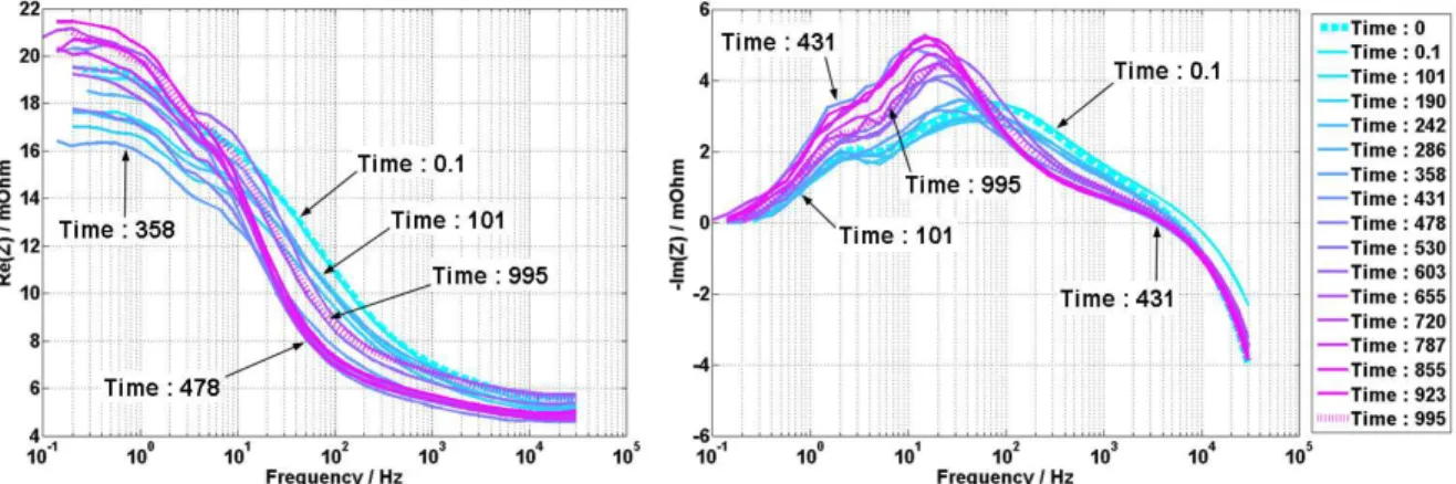
With an explicit point of view, each EIS spectrum could be split into a real part and an imaginary part function of the frequency (see Fig. 5). An inherent link can be established between the FC ageing phenomenon and the evolution of these curves. Therefore, it seems interesting to extract features from these plots that can be used afterwards to estimate the ageing time of the FC stack.

Fig. 5 - Evolution of the real and imaginary parts of the impedance spectrum versus frequency for FC1 from the initial state (Time : 0) to the final state (Time : 995 h).

Feature extraction on the real part of the impedance:

The real part of the impedance can be approximated by an external model of four parameters related to an extended “logsig” function and defined as follows:

(2)

The four model coefficients are determined by minimizing a cost function based on a mean square error with the help of simplex method [12].

Feature extraction on the imaginary part of the impedance:

Rather than using a global fitting of the imaginary part of the spectrum, the idea that we investigate is to automatically partition it into different segments that can be approximated individually by a polynomial. The number of segments is chosen in relation with the physical behavior of the FC stacks while their location and polynomial coefficients are determined by a probabilistic-model-based approach. Further details can be found in [7,8,19]. But the following summarizes this approach.

This feature extraction is made up of a specific regression model that incorporates 3 polynomial regimes (see Section 3.2), and the switching from one regime to another is controlled by a latent variable zi.

More formally, if is the n points of imaginary part of an impedance spectrum obtained for the frequencies (f1,..., fn) (fi will denote the logarithm of the frequency), then the

model can be written as:

(3) Where:

is a discrete variable representing the class label of the polynomial regression mode (K=3),

is the regressor vector associated with , is the variance coefficient associated with .

From this equation, it can be proven that each variable xi is distributed according to a mixture

(4) Where:

is the logistic transformation of the frequency , such that:

(5)

and is the parameter vector of the logistic process.

The model parameters to be estimated are ), where is the vector of coefficients of the polynomial approximating segment i. In order to estimate these parameters, the likelihood function of is maximized with a dedicated EM (Expectation-Maximization) algorithm [20,21]. In addition, the parameters of the hidden logistic process, in the inner loop of the EM algorithm, are estimated using a multi-class Iterative Re-weighted Least-Squares (IRLS) [22]. Figure 6 illustrates the behavior of the modeling where the three domains are clearly identified.

Fig. 6 - Original signal, the three polynomials (top), and their corresponding logistic probabilities (bottom) for the parameterization of EIS imaginary part.

5. Feature selection

The aim of feature selection is to choose a subset of relevant features from the previously extracted ones that retain most of the information about the FC ageing and simultaneously suppress the main part of the "inevitable" model noise. This step is an important part of the

approach because it enables us not only avoiding overfitting and noise disturbance, but it can also reduce computation time of the operating time estimation. That is why different methods were carefully explored, in order to get the best possible results.

To find the optimal subset of features would require computing an exhaustive search, i.e. an evaluation of all the possible subsets of features by training its associate regressor, and then selecting the subset that provides the best performance in terms of operating time estimation. However, given the fact that the number of extracted features is relatively high when both EIS measurements and polarization curves are considered, an exhaustive search would lead to too high computational costs. In order to guarantee the best possible result despite the use of a non-optimal feature selection method, three different subnon-optimal feature selection methods were considered in addition to the exhaustive search:

− the Sequential Forward feature Selection (SFS) starts with an empty feature set (E0 =

∅ (empty set)), adds one feature at a time (Xi), and at each stage chooses the feature

whose addition gives the best performances in terms of the performance criterion J [23].

Begin {

Initialization: E0 = ∅ (empty set), E = { Xi , i = 1 ... D } for each step k = 1 ... D:

- evaluate J{ Ek-1 ∪ Xi } for all Xi∈{ E-Ek-1 } find J(Ek) = min J{ Ek-1 ∪ Xi }

return Ek = { Ek-1 ∪ Xi / J(Ek) } end }

− the Sequential Backward feature Selection (SBS) procedure starts with the entire feature set (E0 = E (full set)) and at each step k drops the feature whose absence less

penalizes the criterion J [23].

Begin {

Initialization: E0 = E (full set), E = { Xi , i = 1 ... D } for each step k = 1 ... D:

- evaluate J{ Ek-1 - Xi } for all Xi∈{ Ek-1 } find J(Ek) = min J{ Ek - Xi }

return Ek = { Ek-1 - Xi / J(Ek) } end }

− the Adaptive Branch and Bound (ABB): the ABB developed by S. Nakariyakul [24,25], is an improvement of the basic branch and bound (BB) algorithm by P. Narendra and K. Fukunaga [23]. Considering the selection of d features from an initial set of D, the BB-type algorithms look for the subset of features by partially scanning the "solution" tree from top to bottom with the possibility of backtracking. Each node of the tree corresponds to a discarded feature. Compared with the basic BB algorithm, the improvements are: (1) the ordering of the tree nodes by significance of the features during the construction of the tree, (2) the selection of the initial bound by a floating search method, (3) a starting search level other than the top of the tree, and (4) the

introduction of an adaptive jump search that selects search levels and avoids redundant calculations. More details can be found in [24,25].

The basic BB algorithm

zi: variable's index, that takes values in [1,...,D].

Begin {

Step 1: Initialization: set initial bound B = -∞, Level i = 1, z0 = 0 Step 2: Generate successors

Initialize List(i) = { zi-1+1, zi-1+2, ... , d+i }, i = 1 ... (D-d) Step 3: select a new node

if List(i) is empty go to step 5. Otherwise set zi = k where

Delete k from List(i) Step 4: check bound:

if ,

go to step 5

if level i = D-d go to step 6. Otherwise, set i = i+1 (advance to new level) and go to step 2. Step 5: backtrack to lower level

Set i = i-1, if i = 0, terminate the algorithm, otherwise, go to step 3 Step 6: last level

Set:

, and go to step 5

end }

6. Test procedure for the operating time estimation

The final step of this estimation phase is the evaluation of the performances of the linear regression model. A cross validation is used. Because of the small size of the data (29 impedance spectra and 29 polarization curves), a particular cross-validation technique, known as the “leave-one-out” technique is carried out as follows [11,26]. Consider the data made up of N elements. The model is trained using (N-1) elements (the training set), and tested on the Nth element (the test set). The process is repeated until each of the N elements is used as a test set. The error rate is then estimated by computing the average of the N resulting test errors. This computation of the error rate will give us an estimation of how well the regression will perform on a new data. In the case of a linear regression, the mean square error as the error rate is used. The “leave-one-out” technique is generally expensive in time computation but it must be used in our case because the data set is very limited. A simple linear regression is achieved for the operating time estimation

7. Results

With the following experiments, the capability of the proposed approach to estimate the operating time using the extracted features can be illustrated. The performances are evaluated on a real dataset made up of 29 impedance spectrum measurements and 29 polarization curves carried out on two FCs (FC1 and FC2 as previously described in Section 3) during 1000 hours of operation time. The feature extraction methods detailed above were applied on the impedance spectra and the polarization curves. These lead to the extraction of variables:

− 6 hyperparameters: the internal resistance (h1), the polarization resistance (h2), the minimal

value of the imaginary part of the spectrum (h3) and its corresponding real part (h4), and the

respective frequencies corresponding to the internal resistance (h5), and the peak of the

spectrum (h6),

− 4 features from the real parts: {ai}1≤i≤4,

− 14 parameters from the imaginary parts: {βi,j, f1, f2}1≤i,j≤4 (3 hidden logistic process

regressions with 12 coefficients of the three-order polynomial fitting of the curve and the 2 frequencies delimiting the central polynomial),

− 5 parameters from the polarization curve model {U0, α1, α2, α3, α4}.

The total number of initial extracted features is therefore 29. The next step of the procedure goes as follows. First, the estimation of the FC operating time is done using EIS spectra and polarization curves separately and while applying each feature selection method. Then, the two sources of information are combined (EIS spectra and polarization curves) and likewise, the estimation is done while applying each feature selection method. These different evaluations are performed in order to highlight the relevance of combining the information extracted from both EIS measurements and polarization curves. The parameter combinations are evaluated in terms of the mean square error of the operating time. At the end of each learning phase, the chosen combination is the one that leads to the minimal rate of the mean square error on the test set.

7.1 Results of the estimation of the FC operating time when using ABB as feature selection method

The use of the ABB algorithm for the feature selection has led to the selection of a subset of 24 parameters to estimate the operating time. These parameters correspond to all the parameters except β11 (the constant value in the first polynomial of the impedance imaginary part, in low

frequencies), β24 (the value affected to the cubic term of the second polynomial of the

impedance imaginary part, in medium frequencies), a3 (of the impedance real part), U0 (the FC

voltage for a zero load current), and α3 (the quadratic term of the polarization curve model).

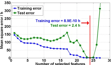
Figure 7 illustrates the distribution of Mean Square Error (MSE) over all the operating time estimation among the database versus the number of selected parameters. In order to see more clearly the evolution of the MSE, a zoom has been performed (leaving the results obtained for a number of selected features of 28 and 29 out of the figure, because the resulting MSEs in these cases are far higher than otherwise). On this figure, one can observe that the operating time of the FC can be estimated with a mean square error of 2 hours over the total duration of 1000 hours. Moreover, we can see that two spikes appear on the test error curve. In most problems, the test error typically decreases then increases, thus a minimal test error appears. This minimal error is used as an indication that from that point when increasing the complexity, the chosen model may be overfitting the data [12]. However, the modeling of the noise could make appear spikes on the test data, as shown in Fig. 7 (for the numbers of selected features equal to 17 and 20).

Fig. 7 - Operating time estimation over the training and the test sets for the linear regression when using the ABB algorithm for feature selection.

7.2 The other results

Table 1 presents the results obtained on the whole dataset for the different feature selection methods that were exploited, and Table 2, the number selected features per selection method. In Table 1, in each feature selection method, there are two sub-columns, presenting the results for the training set and the test set respectively.

Table 1 - Model estimation of the FC operating time (in hours) using different input descriptors and different feature selection methods.

Feature selection method Exhaustive search SFS SBS ABB Training set Test set Training set Test set Training set Test set Training set Test set Polarization curves 131.5 144.1 131.5 144.1 131.5 144.1 131.5 144.1 EIS spectra 51.3 95.0 81.39 152.68 76.6 106.9 68.8 103.8 EIS spectra + polarization curves − − − − 101.3 125.7 7.8E-12 29.9 8.9E-10 2.4

Table 2 - Presentation of the number of selected features per selection method. Feature selection method Exhaustive search SFS SBS ABB Polarization curves 2 2 2 2 EIS spectra 13 12 8 9 EIS spectra + polarization curves − − 6 25 24

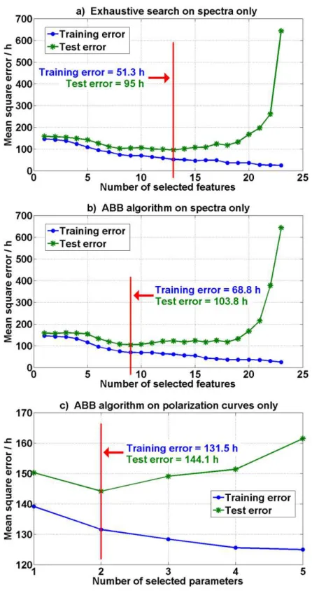
Overall, it can be seen that the training error decreases when the number of selected parameters for the estimating model increases (see Fig. 8). This shows that the more complex the model is, the more it tends to learn correctly the data. Hence, the lower the training error is. However, an overly complex model for the regression could model the noise, and therefore poorly perform on the test set. This is why the test error decreases first and then increases. The point, which corresponds to the minimal test error, gives a trade-off between accuracy and complexity. Moreover, one can observe that for the polarization curves only (i.e. for a small number of initial features), all the 4 feature selection methods give the same (optimal) results. For larger numbers of features, the best results are obtained with the branch and bound algorithm. But

these results remain suboptimal: indeed the results obtained by the ABB algorithm are not as good as the ones obtained with the exhaustive search (see results for the estimation using EIS spectra only in Fig. 8). Given these observations, one can conclude that despite their sub-optimality, the feature selection methods that were used (SFS, SBS, and ABB) have given results that are close to the optimal ones, in the cases of larger initial feature sets. Moreover, it can be noted that it is the combination of features extracted from both the polarization curves and the impedance spectra that gives very good results, even though the number of selected features in that case is high. As one can see in Table 1 and Fig. 8, the results obtained with features from impedance spectra and polarization curves separately are not as good the previously presented results. One can therefore conclude that better results are obtained by combining both the static and dynamic characterizations (i.e. both the polarization curves and the impedance spectra): with this combination of static and dynamic information, the estimation of the operating time (respectively of the ageing time) can be done with a mean error of 2.4 hours on the test set.

Fig. 8 - Operating time estimation over the training and the test sets for the linear regression when using respectively the exhaustive search on spectra only (a)), the ABB algorithm on

spectra only (b)), and the ABB algorithm on polarization curves only (c)).

7.3 Portability of the method

In order to investigate the feasibility of the approach presented here on other FC types, the methodology was applied on a smaller dataset extracted from a different PEMFC type [27]. This FC (noted here FC3) is five cell stack of 600 W assembled with graphite gas plates, commercial membranes and GDLs. It was operated during 1000 hours under nominal

conditions, with the load current constant and equal to 250 A. The polarization curves were recorded in a similar way to FC1 and FC2. For the EIS measurements, the FC polarization point was set to 150 A, and a small sinusoidal alternating part (with amplitude of +/-25 A and frequency range from 10 mHz to 30 kHz) was applied around it [27]. These characterizations enabled us to produce a data set of 8 spectra and 8 polarization curves. The same methodology was then applied to this dataset. Table 3 presents the results obtained on the whole dataset for the different feature selection methods that were exploited, and Table 4, the number of selected features per selection method.

Table 3 - Model estimation of the operating time (in hours) using different input descriptors and different feature selection methods applied on FC3.

Feature selection method SFS SBS ABB Training set Test set Training set Test set Training set Test set Polarization curves 61.34 187.6 65.18 136.9 65.18 136.9 EIS spectra 9.9 42.67 3.74E-13 40.04 1.7E-12 3.28 EIS spectra +

polarization curves

1.38E-12 2.68 1.36 12.9 1.38E-12 2.68

Table 4 - Presentation of the number of selected features per selection method. Feature selection method SFS SBS ABB Polarization curves 4 2 2 EIS spectra 5 12 9 EIS spectra + polarization curves 6 20 6

These results show that the pattern-recognition-based approach could be applied on another type of FC. Interesting results are obtained. Indeed, with this data, we also have an estimation of the operating time with a mean error less than 3 hours.

8. Conclusion

A method to estimate the operating time of FCs, using a pattern-recognition-based approach on both EIS measurements and polarization curves, has been presented in this article. In a previous paper, the same approach was exploited using only EIS measurements. The idea that was investigated here is the possibility of improving the operating time estimation when both EIS measurements (dynamic characterizations) and polarization curves (static characterizations) are exploited. This involves two methods for feature extraction from the impedance spectra, the using of an empiric model for feature extraction on polarization curves, a feature selection procedure to keep only relevant descriptors and a regression model. Because of the size of the set of extracted features, different suboptimal feature selection methods were exploited to ensure that the obtained results were as close to the optimal solutions as possible. Evaluations on real data set have shown that FC operating time (respectively remaining lifetime) can be estimated with a mean error as low as 2 hours over a global operating duration of 1000 hours. This shows an improvement of the results, compared with those obtained previously with EIS measurements only (a mean error of 95 hours over a global operating duration of 1000 hours), and despite the use of suboptimal methods for feature selection.. Moreover, the results we have obtained when using another type of FC show a possible applicability of the method on various

types of FC stacks. Nevertheless, this will have to be validated on more data. These results could lead to interesting perspectives, particularly in preventive maintenance context.

9. References

[1] F. Harel, X. François, D. Candusso, M.-C. Péra, D. Hissel, J.-M. Kauffmann, PEMFC durability test under specific dynamic current solicitation linked to a vehicle road cycle, Fuel Cells 7 (2) (2007), pp. 142–152.

[2] B. Wahdame, D. Candusso, X. François, F. Harel, M.-C. Péra, D. Hissel, J.-M. Kauffmann, Comparison between two PEM fuel cell durability tests performed at constant current and under solicitations linked to transport mission profile, Int. J. Hydrogen Energy 32 (17) (2007), pp. 4523-4536.

[3] M. Ciureanu, R. Roberge, Electrochemical Impedance Study of PEM Fuel Cells. Experimental Diagnostics and Modeling of Air Cathodes, J. Physical Chemistry 105 (2001), pp. 3531-3539.

[4] W. Merida, D.A. Harrington, J.M. Le Canut, G. McLean, Characterisation of proton exchange membrane fuel cell (PEMFC) failures via electrochemical impedance spectroscopy, J. Power Sources 161 (2006), pp. 264-274.

[5] E. Laffly, M.-C. Péra, D. Hissel, Polymer Electrolyte Membrane Fuel Cell Modelling and Parameters Estimation for Ageing Consideration, IEEE ISIE (International Symposium on Industrial Electronics)(2007), pp. 180–185.

[6] J.-H. Lee, J.-H. Lee, S.-H. Kim, W. Choi, K.-W. Park, H.-Y. Sun, S. Choi, J.-H. Oh, Development of a method to estimate the lifespan of PEM fuel cell using electrochemical impedance spectroscopy, J. Power Sources 195 (2010), pp. 6001–6007.

[7] R. Onanena, F. Chamroukhi, L. Oukhellou, D. Candusso, P. Aknin, D. Hissel, Estimation of fuel cell life time using latent variables in regression context, 8th International Conference on Machine Learning and Applications (ICMLA), Miami, 2009.

[8] R Onanena, L. Oukhellou, D. Candusso, A. Samé, D. Hissel, P. Aknin, Estimation of fuel cell operating time for predictive maintenance strategies, Int. J. Hydrogen Energy 35 (15) (2010), pp. 8022-8029.

[9] Y. Tsujioku, M. Iwase, S. Hatakeyama, Analysis and modelling of a direct methanol fuel cell for failure diagnosis, IEEE IECON Conf., Busan, Korea, 2004.

[10] D. Hissel, D. Candusso, F. Harel, Fuzzy Clustering Durability Diagnosis of Polymer Electrolyte Fuel-Cells dedicated to transportation applications, IEEE Trans. on Vehicular Technology 56 (2007), pp.2414-2420.

[11] R. E. Bellman, Adaptive Control Processes: A Guided Tour. Princeton University Press, NJ, 1961.

[12] R. O. Duda, P. E. Hart, D. G. Stork, Pattern classification (2nd ed.), John Wiley and Sons, 2001.

[13] F. Barbir, Fuel cells: Theory and practice, Elsevier Academic Press, New York, 2005. [14] L. Zhang, Y. Liu, H. Song, S. Wang, S.J. Hu, Estimation of contact resistance in proton membrane fuel cell, J. Power Sources (2006) 162, pp 1165-1171.

[15] X. Yuan, H. Wang, J. Colin Sun, J. Zhang, AC impedance technique in PEM fuel cell diagnosis - A review, Int. J. Hydrogen Energy 32(17) (2007), pp. 4365-4380.

[16] M. A. Rubio, A. Urquia, S. Dormido, Diagnosis of performance degradation phenomena in PEM fuel cells, Int. J. Hydrogen Energy 35(7) (2010)), pp. 2586-2590.

[17] X. Yan, M. Hou, L. Sun, D. Liang, Q. Shen, H. Xu, P. Ming, B. Yi, AC impedance characteristics of a 2 kW PEM fuel cell stack under different operating conditions and load changes, Int. J. Hydrogen Energy 32 (17) (2007), pp. 4358-4364.

[18] S. Didierjean, O. Lottin, F. Lapicque, J. Ramousse, M. Boillot, D. Maillet, Forces et faiblesses de la pile à membrane échangeuse de protons, Bulletin de la Société Française de Physique 149 (2003) , pp. 6-9. [in French].

[19] F. Chamroukhi, A. Samé, G. Govaert, P. Aknin, Time series modeling by a regression approach based on a latent process, Neural Networks 22, (5-6) (2009), pp. 593-602.

[20] G. J. McLachlan, D. Peel, Finite mixture models, Wiley series in probability and statistics, New York, 2000.

[21] A. P. Dempster, N. M. Laird, D. B. Rubin, Maximum likelihood for incomplete data via the EM algorithm, Journal of the Royal Statistical Society, Series B, 39 (1977), pp.1-38.

[22] P. Green, Iteratively Reweighted Least Squares for Maximum Likelihood Estimation, and some robust and resistant alternatives, Journal of the Royal Statistical Society, Series B, 46 (1984), pp.149-192.

[23] K. Fukunaga, Introduction to Statistical Pattern Recognition (2nd edition), Academic Press Inc., New York, 1992.

[24] S. Nakariyakul, D. Casasent, Adaptive branch and bound for selecting optimal features, Pattern Recognition Letters 28 (2007), pp. 1415-27.

[25] D. Casasent's homepage: http://www.ece.cmu.edu/~casasent/

[26] C. M. Bishop, Pattern recognition and machine learning, Springer, 2006.

[27] B. Wahdame, L. Girardot, D. Hissel, F. Harel, X. François, D. Candusso, M.-C. Péra, L. Dumercy, Impact of power converter current ripple on the durability of a fuel cell stack, IEEE International Symposium on Industrial Electronics 2008 (ISIE 2008), pp. 1495-1500.