A fictitious domain method for lithosphere-asthenosphere interaction: Application to periodic slab folding in the upper mantle

OATAO is an open access repository that collects the work of Toulouse

researchers and makes it freely available over the web where possible

Any correspondence concerning this service should be sent

to the repository administrator:

tech-oatao@listes-diff.inp-toulouse.fr

This is an author’s version published in:

http://oatao.univ-toulouse.fr/27549

To cite this version:

Cerpa, Nestor G. and Hassani, Riad and Gerbault, Muriel and Prévost,

Jean-Herve A fictitious domain method for lithosphere-asthenosphere interaction:

Application to periodic slab folding in the upper mantle. (2014) Geochemistry,

Geophysics, Geosystems, 15 (5). 1852-1877. ISSN 1525-2027

10.1 002/2014GC0052 41 Key Points:

• Fluid solid coupling method • Uthosphere asthenosphere

interaction

• Periodic slab folding on the 660 km discontinuity

Correspondence to: N.G. Cerpa,

nestor .cerpa@geoazur.unicef r

Citation:

Cerpa, N. G. R Hassani, M. Gerbault, and J. H. Prévost (2014), A fictitious domain method for lithosphere asthenosphere interaction: Application to periodic slab folding in the upper mande, Geochem. Geophys. Geosyst., 15, 1852 1877,doi:10.1002/ 2014GC005241.

A fictitious domain method for lithosphere-asthenosphere

interaction: Application to periodic slab folding in the

upper mantle

Nestor G. Cerpa1_{, Riad Hassani1, Muriel Gerbault} 1_{, and Jean-Herve Prévost}2

1Géoazur, UMR 7329, CNRS, IRD, Observatoire de la Côte d'Azur, Université de Nice Sophia Antipolis, Valbonne, France, 2Department of Civil and Environmental Engineering, Princeton University, Princeton, New Jersey, USA

Abstract

We present a new approach for the lithosphere-asthenosphere interaction in subduction zones. The lithosphere is modeled as a Maxwell viscoelastic body sinking in the viscous asthenosphere. Both domains are discretized by the finite element method, and we use a staggered coupling method. The interaction is provided by a nonmatching interface method called the fictitious domain method. We describe a simplified formulation of this numerical technique and present 2-D examples and benchrnarks. We aim at studying the effect of mantle viscosity on the cydicity of slab folding at the 660 km depth transition zone. Such cyclicity has previously been shown to occur depending on the kinematics of both the overriding and subducting plates, in analog and numerical models that approximate the 660 km depth transition zone as an impenetra­ ble barrier. Here we applied far-field plate velocities corresponding to those of the South-American and Nazca plates at present. Our models show that the viscosity of the asthenosphere impacts on folding cyclidty and conseq uently on the slab's dip as well as the stress regime of the overriding plate. Values of the mantle viscos­ ity between 3 and 5 X 1020 _{Pa s are found to produce cycles similar to those reported for the Andes, which} are of the order of 30-40 Myr (based on magmatism and sedimentological records). Moreover, we discuss the episodic development of horizontal subduction induced by cyclic folding and, hence, propose a new explana­ tion for episodes of fiat subduction under the South-American plate.

1. Introduction

Seismic tomography provides a present-day image of subducting plate geometries throughout the Earth's mantle [Rubie and Van der Hifst, 2001; Fukao and Obayashi, 2013). Analytical studies have unraveled the primary driving forces and parameters that contrai such geometries [e.g., Forsyth and Uyeda, 1975), yet many variations remain unexplained. ln order to fully understand the dynamics of subduction zones, their temporal evolution can only be tackled with numerical, analog, and statistical approaches. Current subduction zone data such as plates velocity, trench motion, back-arc deforrnation, and slab dip were gathered in order to reveal statistical correlations between these parameters [Jaffard, 1986; Heuret and Lallemand, 2005; Lallemand et al., 2005). Heuret and Lallemand (2005) found a general relationship between upper-plate velocity and back-arc deforma­ tion. Nevertheless, they pointed out a potential role of mantle flow in the relative motions between subducting and overriding plates, and the forces acting on them. Asthenospheric flow data being pooriy constrained, mod­ eling studies complement our understanding of asthenosphere-lithosphere interactions in subduction zones. Without disregarding the importance of analog models, we focus here on numerical models. Such models are numerous and can be classified according to their main assumptions. Sorne consider a mantle convection

approach, whereby the dynamic system is mainly controlled by slab-pull, which drives the sin king of the sub­ ducted slab deeper into the mantle [Stegman

et

al., 2006; Morra and Regenauer-Lieb, 2006; Capitanio et al.,

201 O; Stegman

et

al., 201 O; Li and Ribe, 2012). Others consider a plate tectonic approach, whereby kinetic condi­ tions constrain lithospheric displacements [Christensen, 1996; Shemenda, 1993; Cizkova et al., 2002; Zlotnik

et

al., 2007; Gibert et al., 2012). Our approach for modeling the dynamics of subduction zones belongs to this second class and is similar to that of Hassani et al. (1997) and Gibert et al. (2012). Boundary kinematic conditions are imposed at the far edges of the plates, and a density contrast between the lithosphere and the underneath mantle generates the slab-pull. The interaction between the subducting and the overriding plates is modeled, as well as the interaction with an impenetrable discontinuity at 660 km depth separating the upper and lower mantle. Nonetheless, Hassani et al. (1997) and Gibert et al. (2012) have not taken into account the mantle

viscous drag because of the numerical difficulties in coupling the physics of two rheologically different deform­ able bodies. The present study was motivated by the aim to test the role of mantle viscosity on their results. Subduction dynamics, like other geodynamic problems, can be viewed as a competent body embedded in a more deformable medium. From a mechanical point of view, modeling this solid-fluid interaction requires coupling of two physically distinct domains. Usually this kind of problem, which is widespread in many fields (industry, biomedical research, civil engineering, etc.), is solved with common discretization methods, such as the Finite Element Method (FEM), Finite Differences, or Finîtes Volumes, which allow to salve partial differential equations (PDE) in an approximated form.

lntuitively, we could consider the exact discretization of both domains in order to salve the interaction problem, i.e., we have to fit as well as possible the shape of the interface between the two domains. This strategy was used in Bonnardot et al. [2008a) for the lithosphere-asthenosphere interaction, where the fluid and the solid domains are exactly meshed and their joined discrete problem is solved with FEM. As a conse­ quence, the solid's displacements (and deformation) lead to fluid mesh distortion, and a remeshing tech­ nique is needed. This last procedure is computationally expensive. Moreover, in a subduction context, the lithosphere is submitted to large deformation and can acquire a complex geometry [e.g., Gibert et al., 2012). To alleviate the precise meshing of complex geometries, numerical modelers have developed the so-called Fictitious Domain Methods (FDM), also known as "domain embedding methods,' whose name was intro­ duced by Saul'ev [1963). The first application of these methods in fluid-solids problems was credited to Peskin [1972) who modeled heart blood flow. The main idea is to extend the initial problem to a bigger (and simpler) domain, aiming for a simpler mesh to salve the given PDE discretized problem. Generally, the initial domain is "embedded" in a Cartesian grid. Many FDM have been developed to salve ail types of phys­ ical problems. ln fluid modeling (Stokes or Navier-Stokes), one can quote the immersed boundary method

[Peskin, 1972; Lai and Peskin, 2000), the immersed interface method [LeVeque and Li, 1994), the fat boundary method [A.1aury, 2001), the Lagrange multiplier fictitious domain [Glowinski et al., 1995), and the distributed Lagrange multiplier method [Glowinski et al., 1999). To our knowledge, these kinds of solid-fluid coupling methods have not yet been used in geodynamics. Thus, starting from the Lagrange multiplier fictitious domain, we propose here a simple formulation of a nonmatching interface method.

We developed this new fluid-solid coupling method, using the finite element code ADELI for the solid prob­ lem [Hassani et al., 1997; Chéry et al., 2001) and another standard FEM solver for viscous flow, in order to explore the influence of mantle viscosity on subduction cyclicity. Such cyclicity was revealed by numerical [Gibert et al., 2012) and analog [Heuret et al., 2007) models to depend on a specific relationship between plate kinematics, e.g., far-field velocities of the overriding and subducting plates. Other analog and numeri­ cal models simulating freely sinking plates have also produced slab folding on the 660 discontinuity, depending on plate-mantle viscosity and thickness ratios [Schellart, 2008) or on the Stokes buoyancy and effective viscous rigidity of plates [Stegman et al., 2010). ln the present study, we only aim at validating our method and at testing the effect of mantle viscosity on the results obtained by Gibert et al. [2012), for a given set of plate density, rheology, and thickness. The assessment of ail rheological parameters and bound­ ary conditions that contrai the dynamics of subduction zones remains out of our present scope.

This paper is structured as follows. First we recall the mechanical and numerical formulations of both the sol id and the fluid modeling approaches. We detail in section 3 the coupling problem in continuous and discrete terms and present our new simplified fictitious domain method. ln section 4, we present some benchmarks and examples. Then, in section 5, we present our parametric study of the effect of mantle viscosity on subduc­ tion cyclicity taking as example the kinematic conditions corresponding to the Andes. ln section 6, we briefly discuss our results with respect to •tree subduction" scaling analyses. We propose that subduction cyclicity may explain repeated episodes of flat subduction observed along the Andes and how it may also potentially retroact on far-field plate motion. Finally, we present our condusions and prospects for future work.

2. Mechanical Modeling and Numerical Formulation

As in Moffa and Regenauer-Lieb [2006) and Bonnardot et al. [2008b), the lithosphere-asthenosphere system is viewed as a solid-fluid interaction problem where, for reasonable viscosity contrasts, the lithospheric plates behave as sol id bodies which are partially or totally immersed in a viscous fluid, namely, the

Hum

g

I

unilateral contact with friction

vn - -vop ♦ _{vn - -v"'}

-..J•1r"'�,,....---,,;;,.---,,.---..,..,.1..__

=:::r,,

P1,E.TJ1 � p,,E_,1₇₁

I

_{e �::::::}

@

@

y Pa,Tja

Figure 1. Physical model at initial time with boundary conditions on the sol id. The upper mantle lower mande boundary is modeled as an impermeable barrier on which the slab will anchor with a sufficiently high friction. Plate boundary velocities are expressed in reference to this bottom boundary, and positive values of v.., and Vsp correspond to trenchward motion.

asthenospheric mantle. ln this first section, we provide the governing equations which are used to mode) the mechanical evolution of each solid and fluid domain and how both interact. We will further detail the fluid-solid interaction in section 3, which is the technical novelty of the present paper.

2.1. Governing Equations

2.1.1. Solid Lithospheric Plates

The governing equations for the quasistatic evolution of lithospheric plates occupying a physical domain Q c 11?2 _are

{

diva+p₁g=O in Q,,

�; =M(a,d) in

n,,

(1)

where <J is the Cauchy stress field, gis the vector of gravity acceleration, p1 is lithospheric density, d ½ (v'li+ v'lir)

is the Eulerian strain rate tensor, and

li

the velocity field. Da/ Dt stands for an objective time derivative and M rep­ resents a general constitutive law. We assume in this study a simple elastic or viscoelastic Maxwell behavior

G

M(a,d)=2Gd+ltrdl -deva (2)

,.,

where tr and dev are, respectively, the trace and deviatoric parts of a second-order tensor, / is the identity tensor, À. and Gare the Lamé parameters, and 17 is the viscosity coefficient.

Moreover, plate-plate and plate-rigid foundation interactions are modeled with the following conditions:

{

ôÙn $ 0, /Jn $ 0, ôÙn<Jn l11rl :::; µ11" if oùr o ôÙt

• •

<Jr 1111 n _lôùrl if ôUr / 0 0 on

r,,

on

r,,

on

r,,

(3)

where ôÜn and Our are, respectively, the normal and tangential components of the relative velocity between two points in contact and µ is the friction coefficient. The normal components on the contact interface r, are computed according to the outward normal vector. The first line of the equation (3) corresponds to the Signorini relations (no interpenetration, no attraction, and complementary condition) while the two remain­ ing lines describe the Coulomb friction law. ln addition, boundary conditions are imposed as velocity or stress components on parts of the solid domain boundary ôQ1• Figure 1 summarizes the solid model.

2.1.2. Fluid Asthenospheric Mantle The stationary Stokes problem

{ div� Vp+p0g=O in

no,

is used to compute, at a given time t, the velocity field v, the pressure p, and the viscous stress -r 11aC'vv+ 'vvT_{) in the fluid domain}

n.,,

_{knowing the viscosity 'la, the density Pa, and a set of boundary conditions. The} latter are expressed as velocity or stress components on a portion of the boundary of the fluid domain

ôil.,.

2.1.3. Solid-Fluid Interaction

The continuity of the traction vector is required (action-reaction principle), on the interface r,a shared by the solid (lithosphere) and by the fluid (asthenosphere). Because of the viscosity, the fluid and the solid are perfectly glued to each other, which also implies the continuity of the velocity field on r,a

{V=

U on r,a,

(-r pl) · n

=a·

n _{on r,a,} (5)

The application of our physical mode) to subduction systems presents the following restrictions, which are planned to be tackled in future work:

Viscosity and density remain constant in time, since thermal effects are ignored (as well as phase transi­ tions). Consequently, our targeted applications are at the moment only valid for subductions zones that are fast enough compared to their thermal diffusion time scale. Viscosity and density also remain constant or piecewise constant in space since matter is not advected.

The upper-lower mantle interface at 660 km depth is modeled as an impenetrable barrier. The mechanism of slab penetration into the lower mantle is thus ignored.

2.2. Num erical Formulation

2.2.1. Solid Lithospheric Plates

An approximate solution to the continuous problem (1-3) is computed using the Galerkin finite element code ADELI. ADELI has been used in numerous geodynamical applications, for processes at the crustal scale [e.g., Huc et al., 1998; Got et al., 2008] as well as at the lithospheric scale [e.g., Hassani et al., 1997; Chéry et al., 2001; Bonnardot et al., 2008b]. This code belongs to the FLAC family of codes [Cundall and Board, 1988; Poliakov and Podladchikov, 1992] and is based on the dynamic relaxation method.

ln order to describe in section 3, our strategy to mode) the solid-fluid interaction, here we recall the time­ discretization of the equilibrium equation (1) used in ADELI. More details about this code, in two and in three dimensions, can be found in Hass ani et al. [1997] and Chéry et al. [2001].

The finite element approximation of the quasistatic equilibrium equation (1) leads to a set of algebraic non­ linear equations of the form

F;nr(Ùqs,

t)

+Fexr(Ùqs,

t)=O

(6)

where Finr, Fexr, and Ùqs, vectors in IR2N' (with N1 the number of nodes in the mesh of�), are internai forces, external forces, and nodal velocities, respectively. ln the dynamic relaxation method [e.g., Underwood, 1983; Cundall and Board, 1988], the quasistatic solution Ùqs is approximated by the solution

Ù

of a pseudodynamic

problem by introducing a user-defined mass matrix M, an acceleration vector

Ü,

and a damping force vector C. The discrete problem becomes

F;nr(Ù, t)+Fexr(Ù, t)=MÜ+C (7)

Thus, when the acceleration and the damping force become negligible compared to the extemal and the internai forces, the quasistatic solution is reached [Cundal/, 1988]. ln addition, this method is coupled with an explicit time marching scheme

Ùn+1/2=Ùn 1/2+tltÜn+1

V'+l =V'+tlt_Ùn+l/2

(8)

where Ü0+1 and V'+1 _{are the nodal acceleration and displacement vectors at time t}0+1 _{t°+tlt, respec­}

tively, tlt is the time step, M 1 is the inverse mass matrix, Ff_nr and F':xr are, respectively, the internai and external forces computed at

f',

and Ù0+112

The term

C

damps the dynamic solution and enforces the convergence toward the quasistatic solution. lt is chosen proportional to the out-of-forces balance, and it must thus vanish at the quasistatic equilibrium

(9) for j 1, 2, • • •, 2N1 and ocd E]O, 1]. ln practice, ocd 0.5 or ocd 0.8 appear to be suitable values [see Cundall,

1988].

2.2.2. Fluid Asthenospheric Mantle

With regards to the classical stationary Stokes problem (4), the Galerkin finite element method with equal­ order interpolant for both velocity and pressure is used. Hence, a stabilized technique based on polynomial pressure projections [Dohrmann and Bochev, 2004; Burstedde et al., 2009] is needed. The fluid domain

n.,

is covered by a triangular or quadrilateral mesh of N0 nodes. The resulting discrete system is of the form

(10)

with V E IR2N_{• the nodal velocities vector, P E !R}N_{• the nodal pressures vector, F E IR}2N_{• the nodal external} forces, and A a symmetric 3N0 X3N0 matrix. Referring to subsequent sections, we can formally express the

nodal velocities vector as the solution of a linear system of the type

KV=Fo, (11)

3. Solid-Fluid Coupling: A Fictitious Domain Method

Modeling the interaction of a deformable structure moving in a fluid presents a number of challenging numerical problems. Among them is the way in which to follow the interface

r,

0 which separates the solid

and the fluid domains, and the resulting change in geometry of the fluid domain.

A first option consists in remeshing the fluid domain and was adopted by Bonnardot et al. [2008a]. However, this approach is arduous to implement, computationally time consuming, and laborious to deal with when the shape of the fluid domain becomes complex, especially in three dimensions. To alleviate meshing or remeshing efforts of complex domains, the Fictitious Domain Method (FDM) has been implemented in many fields for solving the interaction between two bodies of different physical behavior. FDM had initially been developed for the application of boundary conditions on geometrically complex boundaries [Saul'ev,

1963], and in our case, this type of method is also useful to solve the fluid problem on a Cartesian grid. ln the first of the two following subsections, we describe the general formulation of a simplified variation of FDM that we implemented. Then, we detail the numerical strategy adopted to interlock fluid and solid cal­ culations in a stable manner.

3.1. General Formulation

To describe the Fictitious Domain Method (FDM), let us consider a simple linear problem where a scalar physical field vis sought in a domain !20 presenting a hole or an inclusion Q1 of any shape (below we will

also name it an obstacle). We name

r,

0 the boundary of the hole and

r

the external boundary ofil., (see

Figure 2a). Assuming that the value of vis prescribed on

r,

0 and

r

,

C is a given linear differential operator,

and fis a known function, the linear problem is written

{

C(v)=f in

n.,

,

v=_vo on

r,

v=_v,a on

r

_i,

.

(12) ln the standard finite element approach, the boundary condition on

r,

0 requires to define a mesh of

n.,

that matches as best as possible the shape of the obstacle. The main idea of the fictitious domain method is to extend the problem into a geometrically Jess complex domain Q

n.,

u 0/ and to enforce the Dirichlet condition v via on

r,

0 by introducing some source terms in (12) (see Figure 2b).

a r:l'Q V

b

1 1 1 1 1--+---+-Û = Ûa U Ûa--Xl ... ·"·•• .. 'e .r

·

··

•

..

·

·

··

·

•

Figure 2. (a) Scheme of the continuous fluid problem with an 'obstacle.' (b) Scheme of the discrete fictitious domain problem.

ln the absence of the obstacle�. the corresponding discrete finite element expression of the problem takes the form

KV=Fo (13)

where VE IRN _{is the vector of nodal unknowns, F0 E IR}N _{is the vector of nodal loads including the Dirichlet}

boundary condition on r, N is the number of nodes belonging to the mesh of Q, and K is the N X N matrix of rigidity (we suppose K symmetric and invertible).

Now let xk E IR2 (k 1, • • • , n10) be a given set of n10 points forming an independent mesh of the immersed

boundary

r,

0• The finite element approximation of vat each point xk reads

v(xk)=

L

_<P;(xk)V;=_{(Cl>V)k (14)}

i•l

where

<f,;

is the interpolation function at node i, V; is the ith component of

V,

and Cl> is the n,aXN matrix whose entries are the <P;(Xk) values. To ensure v(xk) is close to v,a(Xk) (in a given sense), a source term is added on the right-hand side of (13)

KV=Fo+F(q) (15)

where q is an unknown source function defined on

r,

0•

Since any given v10 distribution may not be consistent with the problem (12) (for instance, in our case the linear problem (12) is the incompressible Stokes problem and v10 corresponds to the velocity of the sol id boundary which, generally, does not conform with the incompressibility constraint), we proceed with a least squares method

n•

minimize J(q) : = L(v(xk) v,a(xk))2=llcI>V v,all2 (16)

k•l where Vis given by (15) and v,0 (v,0(x, ), · · ·, v,0(xn,.)).

The last step consists of choosing the parametrization of the source function q. The simplest way is to

define a ponctuai distribution at the n10 contrai points xk: q(x) I:k qkô(x xk), where ô is the Dirac func­

tion. ln this case, the assembled vector F(q) is simply given by

where q=(q,, • • •, q_,,.,).

Solving the least squares problem (16) for

q

gives the nb xn,a linear system

kq=v,0 Vo

with k Cl>K 1 Cl>r _{and v}

0 Cl>K 1 F0 (which corresponds to the solution of the n10 contrai points in the absence of the obstacle).

(17)

We can make the following remarks:

1. When applied to the fluid-solid coupling problem, the physical field vis _{the fluid velocity vector and} q corresponds to the distributed drag force acting on the immersed sol id boundary r,0• Moreover, if the con­

trai points xk form a subset of the sol id mesh nodes, then the qk values determined by (18) are the corre­ sponding nodal forces.

2. Other parametrizations for q are possible but lead to a slightly more complex implementation. If we choose for example q to take the form q(x) I:k qkV'k

(x),

where V'k are the interpolation functions on the

mesh ofr,0, then the resulting nodal source term has to be computed as F(q) 'l'r _{q, where}

'l'k;

fr

..

r/J;(x)ifl_k(x)dx. Thus, intersections between the mesh of r,0 and the mesh of Q must be computed beforehand at each time. With this variant, our FDM is closely akin to the Lagrange multiplier fictitious domain of Glowinski et al. [1995).

3.2. Numerical Strategy for lmplementing Solid-Fluid Coupling

Severa) approaches exist to tackle problems of fluid-structure interaction [Felippa et al., 2001), ranging from the monolitic ones (in which the solid and fluid subproblems are solved simultaneously as they are formu­ lated in a unique problem) to the staggered ones (in which the subproblems are solved separately and coupled at specific discrete time steps). The second approaches are more flexible since they allow the use of two separate codes and facilitate the use of nonmatching meshes. Our formulation belongs to this sec­ ond kind and uses a semi-implicit time marching scheme for a stability purpose.

We recall that the solid domain Q1 is discretized with a finite element mesh containing N1 nodes (with n10

nodes on its immersed boundary r,0), while the mesh of the fictitious fluid domain Q Q,,

u

Q1 is discretized

with N nodes. At a given time t"+1_{, the solid state is calculated according to (8), in which the force balance}

is modified to account for the fluid reaction F_{10 that acts on the} n10 nodes of the immersed solid boundary

r,0• ln a purely explicit coupling procedure, this reaction is evaluated at the previous time step t", but

unfortunately this easier scheme often tums out to be numerically unstable. The implicit variant improves stability but introduces the unknown reaction Ff/1 at time t"+1_{• A predictor-corrector-type algorithm is}

thus used, as follows. First, the solid nodal velocities vector can be expressed by

where u;:e112 is the predicted nodal velocities vector in the absence of viscous fluid drag

un_Free +1/2=Un 1/2+d _t M l[Fn +Fn

,it ext Equation (19) can obviously be rewritten for the n10 nodes of r,0

en

].

(19)

(20)

(21) where un_+l/l _LÙn+lfl_,

u;;/

2 Lu;;

e112, and Lis a n,axN, Boolean matrix (extraction matrix). The viscous

fluid forces

Ft

1 acting on the solid mesh are given by

(22)

where qn+1 (the source terms) are, according to (18), solution of the linear system

(23) where lc1'+1 _cJ>0+1 _K 1 _cJ>0+1r_{. Let us recall that this system is "small" regarding to the whole grid size, since}

it involves only the contrai nodes of the solid's boundary.

lnserting (23) and (22) into (21), we obtain the corrected velocities by solving the linear system

(24) where mis the nodal mass matrix of the n10 nodes (recall that M _{is diagonal).}

Our coupling fluid-solid procedure can be summarized by the following flowchart:

1. lnitialization: define the meshes of the initial sol id domain

n?

and of the fictitious (fixed) domain Q, define

the initial sol id state (U0_,

ü

0_{, u}0_{) and the initial fluid state (V}0_{, ,}f 0).

2. Assemble and factorize the Stokes matrix

K

of the fictitious problem. 3. New time step: t"+1 _t"+M.

4. Prediction stage: compute the predicted solid velocities u;;e112 from (20).

5. Extract the predicted velocities

11�,:

1

12 at the n10 sol id boundary nodes of

r,

0•

6. Compute the matrix lc"+1 _{and the source terms at the n}

10 contrai points from (23) using the predicted

1 • • _.JJ+l/2 ve ocitIes _ufree

7. Compute the fluid velocities (if desired) by solving the Stokes problem

Kvn+l =Fo+Cl>n+lT q"+l.

8. Correction stage: correct the velocities and positions of the n10 nodes by solving (24). 9. Update the stress c,0+1 _{of the solid and assemble the new internai and external forces Ff}

0

;

1

,

F'::;1, as well

as the fluid-solid interaction by (22).

1 O. n f-n+ 1 and go to 3.

To resume, the main advantages of the FDM are:

1. To avoid repetitive remeshing in the fluid domain (calculations on a fixed mesh).

2. To handle complex geometries and still be able to use a Cartesian mesh, since the fluid domain has a sim­ ple shape.

3. The user can define which points on the solid boundary are coupled with the fluid. "One-way coupling• or ''two-way coupling" is easy to handle. For instance in our applications, the top boundaries of solid plates are chosen to remain as free surfaces. This is an important advantage of our coupling method.

However, FDM also has the following disadvantages:

1. As we will see below, our variant of this method is only first-order accurate.

2. The fictitious domain method is only used for the fluid domain. Thus, the L.agrangian description used to resolve the evolution of solid plates still needs a remeshing technique for very large deformation.

3. For each contrai point in our coupling procedure, we need to compute the product of

K

1 _cJ>r_{, leading to}

a large number of linear systems to solve if their number is important.

4. Benchmarks and Examples

We shall now demonstrate the potential of our new coupling method with a few benchmarks and valida­ tions, in two dimensions. We emphasize that our FDM was also implemented in the finite element analysis program Dynaflow™ _{[Prevost, 1981), and some of the following examples were performed and compared}

with the two codes. We start with the benchmark of an analytical solution for a rigid solid immersed in a fluid (section 4.1) and then move on to problems considering a deformable solid, for which we compare our solution with other numerical solutions (sections 4.2 and 4.3). Then in section 4.4, we tackle the ana log subduction experiment by Guillaume et al. [2009) which was also used as a benchmark in Gibert et al. [2012) and conclude in section 4.5 with a comparison with the community benchmark proposed by Schmeling et al. [2008).

4.1. An Analytical Stationary Solution: The Wannier Flow

As a first validation of our FDM in a 2D stationary case, we consider an analytical solution of Stokes flow problem called the Wannier flow [Wannier, 1950; Ye et al., 1999). lt considers the viscous flow around a rigid cylinder rotating with an angular velocity OJ near a wall in translation (see Figure 3a). The velocity and the

y

î

-

�

-

-

-

·

/

oh

: X

id

u

,oo -1---�-�-�-..._--�---��---''---, e(p) • 10-'

..

.

a=0.61

.

.

.

.

.

e(u).

.

.

.

.

.

.

a=l.04

-..

10-• log(h)

Figure 3. (a) Scheme of the Wannier flow [Wannier, 1950). (b) L2 _{discrete errors of velocity and pressure numerical field as a function of the mesh size h. The slope a of the lines repre}

sents the order of convergence for both the velocity and the pressure. The linear convergence is satisfactory regarding the Ql elements used for the finite element discretization.

with ux=_{U 2(A+Fy) [}s:y + 5

/

]

_Fini 8 _[s+ 2y 2y(s+y)2_] ex ex2 C _{[s p}2y + 2y(�/) 2 ]

uy=2x[(A+Fy)(.!. .!.) s9(s+y) cy(s

y)]

ex p ex2 p2

p

=

11x[B s+y

+c

5

Y +4F sy

]

(K+ys)

2

_{(K ys)}

2

_K

2

y

2

_s

₂

s

=_✓

d

2 _r2_,

y

=

(d+s)/(d

_{s), ,}=_wr2_/2s, A=

d(F+,), 8=2(d+s)(F+,),

_C=_2(d

s)(F+,),

F=_U/lny,

y=y+d,

ex=_x2+(s+y)2_,

_P=x

2

_+(s

_y)2_,

_K(x

2

_+y

2

_+s

2

_)/2

where

x

and y are the Cartesian coordinates in the plane, 17 is the viscosity of fluid, and other geometrical

parameters can be viewed in Figure 3a.

The fluid domain is a square of edge length 1.5 m and is discretized by a regular mesh of size equal

to h. _{We placed at distance intervals} h_{ep a certain amount of contrai points on the boundary of the}

cylinder which is placed at the center of the domain. We impose on the fluid domain boundaries the analytical solution that simulates an infinite medium and we impose the mean pressure to be

equal to O.

We produce a convergence diagram (Figure 3b) in which the analytical and numerical solutions for our ficti­ tious domain method are compared, by computing the L 2 _{discrete error for each field. These results are}

close to those obtained with other nonmatching interface methods [e.g., Ye et al., 1999).

We have performed a number of experiments with different mesh sizes varying the distance hep between contrai points, and we have identified an optimum distance that ranges between 1 and 2 times the grid mesh size. This range is also known in Lagrange multiplier fictitious domain methods [Glowinski et al., 1995).

4.2. Sinking of a Competent Block lnto a Viscous Medium

We consider here the coupling case of two deformable media found in Gerya and Yuen [2003), in which a

competent block of density Ps 3300 kg .m 3 sinks into a viscous medium of density Pr 3200 kg .m 3 and of viscosity IJr 1021 _{Pa .s. The viscous medium is a square domain with edge lengths equal to 500 km, and}

its boundaries are set free-slip. The competent block is a smaller square with edge lengths equal to 100 km, initially placed at a distance of 50 km below the upper edge of the vis cous domain.

The sol id solver ADELI is used for the competent block, whereas another finite element direct solver is used to compute the Stokes flow for the surrounding fluid. The block is viscoelastic with a Young modulus equal to 1011 _{Pa , and three different viscosity values are tested (1J}

5 102

2 _{Pa .s, 10}23 _{Pa .s, and 102}4 _{Pa .s). The Max­} well relaxation time is consequently less than 0.43 Myrs, and the elastic behavior of the block is thus negligible.

Results are displayed in Figure 4. The smaller the viscosity of the block, the more its deformation is impor­ tant The viscoelastic sol id sinks faster at low viscosities because of the "aerodynamic" shape that it adopts. After 1 S and 20 Myr, the height and shape of the block are similar to those displayed by Gerya and Yuen

[2003) for different viscosities. 4.3. Bending of an Elastic Plate

We perform the numerical experiment proposed by Bonnardot et al. [2008a) in order to compare their results obtained with a remeshing coupling technique, with our results obtained with the fictitious domain method.

This two-dimensional numerical experiment consists of an elastic plate of length I 3 m and thickness

e 0.2 m immersed in a fluid channel of width L 6 m. A fluid of viscosity IJ 105 _{Pa s is injected in the}

channel with a prescribed horizontal velocity v 60 m/s. The duration of the experiment is T 1 s. The plate bends until it reaches equilibrium. Figure Sa displays the final pressure and velocity vectors in the fluid.

ln Bonnardot et al. [2008a), both the solid and the fluid domains were discretized with unstructured meshes that match exactly at their interface. Periodic remeshing of the fluid domain was needed during the evolu­ tion due to the solid motion. The solid's boundary velocity was imposed as a Dirichlet condition to the fluid mesh.

We display in Figure Sa the pressure field when the static solution is reached. The bent plate is represented in gray and some of its intermediate positions are drawn in dashed gray line. For comparison, we show in Figure Sb the evolution of the displacements of the bottom-left corner of the plate obtained with our cou­ pling using the fictitious method (solid line) and those obtained with a remeshing technique. Results are similar.

4.4. A Laboratory Test of Subduction by Guillaume et al. [2009]

Numerous analog models have been developed in order to understand different aspects of subduction dynamics. We can class laboratory subduction studies into three classes. The first class considers freely sub­ ducting plate dynamics [Schellart, 2004; Belfahsen et al., 2005), i.e., the system is only driven by the slab-pull force. ln the second class, a kinematic condition is imposed to the far edge of the subducted plate [Funidello et al., 2004), but the upper plate is absent A third class of laboratory experiments includes the application of a plate velocity and also takes into account the upper plate [Heuret et al., 2007; Espurt et al., 2008; Guil­ laume et al., 2009). This last category is the one that we consider with our numerical approach.

ln this section, we aim at reproducing, at the laboratory scale, the reference model of Guillaume et al. [2009), as did Gibert et al. [2012). Although in Gibert et al. [2012) the numerical results were close to those obtained in the laboratory experiment, minor differences had been attributed to the absence of a viscous mantle. With the coupling method presented here, we are able to test the effect of an underiying viscous material.

ln the laboratory experiment, a viscoelastic silicone material was ta ken to simulate tectonic plates. These plates were placed above glucose syrup (mantle) inside a Plexiglas tank. A rigid piston pushed the sub­ ducted plate on the far edge, while the upper plate was held fixed. The bottom of the tank represented the 660 km depth boundary. Parameters are summarized in Table 1. Note that the coefficient of friction

�

0 Il 1-Il 1-!!! >,

�

0 C\I Il 1-'Tlblock = 1.1022 .,

.. . . .. ...

' " .. • ► • ... •

. .. .. . ..

" .,

..

.

..

.

' .. ,.

.. .. . .

" • ... .. .. .. , .. ◄ .. . <I " r ► ._ , .. ., " ► • A

•••

•

•

•

•

• •

.

..

. .

' ... ... "

.

• .. ... ,. ... A' ,,, ., ...

...

- _

__,

-'Tlblock = 1.1023 ., .. • ► .. .. ' .. ◄ .. ... * • .. .. • .. • , .. .. ◄ .. " ...

.. ..

... ' '

, ..

.. ..

..

'

,,

.. ..

... \

.

'

;

.

..

" \ , , ... ,\li_... , , '- \ ' " · '\11"- � ,i I / - _I - ' \ \ 11,.�\

, . ,\\

1 t 1 • 1 _{• 1 ' 1} l\1 , 1

1. , //

,,, .... .,. \-//! ', ... --.- ...__ ___ ,,, JI

.,

.. .. .. ..

.. ◄ .. .. ...

.

.,

. . ..

• .. ... • t ' .. •

: : :: :

..

..

...

..

a:

' ,,,.. ,,, ., .,

.·

· .. :

'llblock = 1.1024 ., .. ► ► ... .. ' • ◄ .. .. • ... .. ... ► ..

.

.. ..

.

..

,

.. .. .. ..

... ., .. ► .. ... , .. .. ◄ .. . . • ., .. .. .. ... 1 ,, .. .... • ., .. ► .. • ,. .. ..

Figure 4. Sinking block benchmark [from Ge,ya and Yuen, 2003). Results for three viscosity ratios •1./•1,: 10, 100, and 1000.

between the plates and between silicone and plexiglass are difficult to quantify precisely in analog models, whereas one must always provide them in the numerical models.

The Dirichlet conditions on the boundary of the fluid domain in the numerical experiment are chosen as fol­ lows: normal and tangential velocities at the bottom and edges boundaries are equal to zero. Because there can be vertical motion of the solid, we cannot assume a free-slip top boundary of the fluid domain at the same depth level as for the solid (problem of consistency of the contrai points' velocities and this boundary condition). Thus, we immerse the solid well below the top boundary of the fluid, in order to safely set the

fluid top boundary as free-slip. Consequently the fluid domain is divided into two. The first main domain

defines the area located in between the bottom of the tank and depth S mm and has the viscosity of the glycose syrup. The second domain extending from depth S mm to +3 mm (the plates' domain is initially

set between O and depth 13 mm) has a weaker viscosity of 10 6 _{Pa .s and a density equal to O. Note that}

we do not account for the viscous drag exerted on the upper boundary points of the solid plates, so that the latter remain free-surfaces ('one-way coupling').

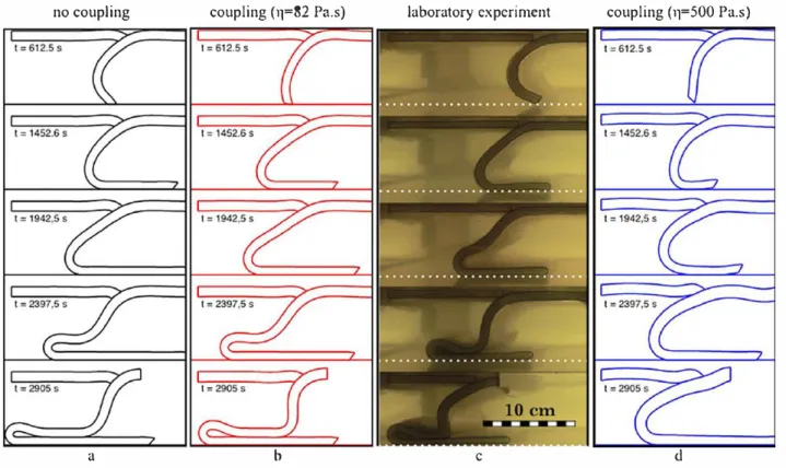
Figure 6 displays the comparison between the numerical results and the laboratory test by Guillaume et al. (2009]. The first column shows the results obtained with an inviscid fluid (no coupling with the fluid solver, similarly to Gibert et al. (2012]). The second col umn displays the result accounting for a fluid of viscosity 82 Pa s equal to that of the glucose syrup used in the laboratory experiment by Gui/laume et al. (2009] (third column). Despite the need to assume an arbitrary friction coefficient in the mechanical models, the numeri­ cal result confirms that the viscous fluid in this experiment has a negligible effect on the slab evolution.

-2 -4

.

. . .

_.

. .

.

.

-4 -2 0 2 4 6

b

1.5

+---�-�--�--�--�-�--�--�-�---1.0

E

0.5 � 0.0 � -0.5 �

a.

-1.0 .!!? -o -1.5 -2.0

---

---

---- ---- ---- ---- Method with remeshing (Bonnardot et al., 2008)

--- This fictitious domain method

-2.5

+---�-�--�--�--�-�--�--�-�---0.0 0.2 0.4 0.6 0.8 1.0

time(s)

Pressure _(MPa) 5.0 1.6 -1.8 -5.2 - -8.6 -12.0

Figure S. (a) Pressure and velocity fields for the experiment of an elastic plate bent by a viscous flow. (b) Displacement of the bottom left corner of the plate over time.

Figure 6d displays the result obtained with a greater value of the ana log mantle viscosity, equal to 500 Pa s, which corresponds to a mantle viscosity of 1021 _{Pa .s at the natural scale. With this viscosity, the modeled}

subducted plate does not fold but rather bends smoothly backward. The viscous drag a long the plate is stronger. Consequently, penetration of the subducted plate is harder and the far-field kinematic boundary condition is accommodated by greater internai deformation than in the analog model. Moreover, the experiment produces a huge arc bulge, unrealistic at the natural scale. Actually, this bulge results from our choice of an arbitrarily high plate interface friction coefficientµ 0.4, which allows to match the internai deformation of the numerical and the ana log models. This value is obviously unrealistic for a subduction interface, and in the following models, we have chosen friction values Jess than 0.1, consistent with those reported in the literature [Cottin et al., 1997; Lamb, 2006).

This experiment with an extreme mantle viscosity of 500 Pa s shows the drastic effect of the underlying mantle viscosity on the subducting plate geometry. The shape of folds is modified and at least, delayed in time. Overriding plate deformation (shortening or extension) is also affected. We will mainly focus on these points in section 5 when studying real scale subduction zones.

4.5. Community Benchmark by Schmeling et al. [2008]

We perform the benchmark test proposed in Schmeling et al. [2008). lt allows to compare our results with those obtained with several others types of codes (finite differences or finite elements, Lagrangian or Euler­ ian). This 2D benchmark consists in the sinking of a competent and dense body (simplified L-shaped plate with a horizontal length of 2000 km) driven only by internai forces into a viscous mantle down to 700 km depth.

Table 1. Mechanical Parameters for the Test Described in Section 4.4• Parameters Plate thickness, e Density contrast, tJ.p=p, Pm Plates viscosity ,,, Subducting plate Overriding plate Young modulus, E POÎsson ratio, v Friction coefficient,µ Plates interface Plate/660 km discontinuity Fluid viscosity, •la

Values Used in the Reference Model 13mm 76kgm-3 5.0 X lo' Pa. 3.0 X lo' Pa.s 5000 Pa• 0.25• OA" 0.02• 82 Pa s Equivalence at the Natural Scale 90km 76 kg.m-3 1.3 X 1o"' Pa.s 7.7 X 1CJ2' Pa.s 4.9 X 1010 _Pa 0.25 0.4 0.02 1.64 X 1020 _Pa.s "The set of parameters marked with • are not evaluated in Guillaume et al. (2009] and have been arbitrarily chosen in order to reproduce as best as possible the laboratory results.

We consider a viscoelastic material for the modeled slab. We assume a Young modulus of 184 GPa and a Poisson ratio of 0.244 corresponding to the values used in the Lapex-2D code (details in Schmeling et al. (2008]). The relaxation time (about 40 Kyr) is very small in comparison to the time of the experiment, and thus the effect of slab elasticity is negligible.

The top surface of the plate is free­ surface and its right-edge is fixed. The other edges of the plate are coupled with the fluid. To avoid big mesh dis­ tortions in the solid, its remeshing is prescribed every 10 Myr. For the fluid domain, the bottom and edges are set free-slip, but for the top boundary we explore four types of conditions (see scheme Figure 7). Type 1 is top-open. ln type 2, the top boundary is free-slip. ln the other two types we add a zero'1ensity layer with a viscosity equal to that of the mantle (type 3) or equal to 1019_{Pa .s (type 4).}

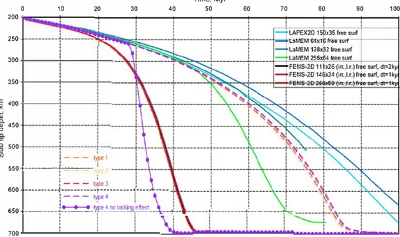
ln Figure 8 our results are compared with those obtained with codes assuming a free-surface in Schmeling et al. (2008] (sol id lines). The vertical position of the slab tip in time is similar for ail four types of boundary conditions tested for the fluid domain (dashed lines). They follow the same slope as experiments using codes LAPEX 2D and LaMEM (coarse meshes) until 45 Myr. These results are obtained, in our case, with the upper-left corner of the slab never sinking into the mantle (similar in its effect to the "numerical-locking" of the wedge described by Schmeling et al. (2008]).

We perform an additional experiment in which we couple the points at the plate's top-surface with the fluid, so that the plate can sink below a threshold depth (Figure 8, purple line with circles). Then, the slope of the sinking slab, from about 30 Myr onward, becomes similar to that obtained without •numerical lock­ ing" at the wedge and with the viscous code FEMS-2D. However, the change in slope always remains more abrupt with our solution. Nevertheless, one must realize that when modeling a realistic subduction zone, this problem is not relevant since an overriding plate is present

ln Figure 8, we note negligible differences in cases with (types 3 and 4) and without (types 1 and 2) the additional zero-density low-viscosity layer. The flow in this layer has no effect on the bulk flow of the man­ tle, and thus on the evolution of the solid domain. Consequently, in our subduction models, we shall incor­

porate this layer only to consistently deal with both the free-slip boundary condition on the fluid and the

free top surface condition on plates (also considered when benchmarking the laboratory experiment).

S. Effects of Mantle Viscosity on Subduction Cyclicity

Evidences for episodic development of the Andean orogeny have been noted for decades. Steinmann et al. (1929] and Mégard (1984] reported episodes of continental shortening separated by periods of relative quiescence. Recently, Folguera and Ramos (2011] identified three fiat slab domains since Cretaceous times in the Southern Andes. ln the Central Andes, a compilation of isotopie and geo­ chronological data by Haschke et al. (2006] showed that arc magmatism migrated every 30-40 Myr since about 100 Myr, leading the authors to propose a link with cyclic episodes of fiat subduction (the latter marking magmatic gaps). Martinod et al. (201 O] also proposed a link between compres­ sional events during the Cenozoic, with periods of increasing plate convergence and fiat subduction in specific areas along the margin.

Haschke et al. (2006] related episodes of horizontal subduction with possibly repeated slab break-offs. Hori­ zontal subduction is also commonly associated to the resisting subduction of a buoyant oceanic plateau. However, the validation of this mechanism remains problematic along the Andean margin (see discussion

no coupling

coupling (TJ=82 Pa.s)

laboratory experiment

coupling (11=500 Pa.s)

a

b

C

d

Figure 6. Comparison between (a, b, d) numerical models and (c) the laboratory result of Guillaume et al. (2009) for different values of the mande viscosity.

in Gibert et al. [2012) and Gerbault et al. [2009)) and with statistics on subducting ridges carried out world­ wide [Skinner and Oayton, 2013).

Here similarly to the previous numerical study by Gibert et al. [2012), we explore another cause for slab dip evolution. lndeed, depending on far-field plate kinematics, the development of slab folding, as it deposits on the 660 km depth boundary, may periodically flatten the slab. If v,p and v0_P refer, respectively, to the sub­ ducting and overriding plate velocities, counted positive toward the trench, cyclic folding was found to occur when lv_opl < v0_p+v.,,, [Gibert et al., 2012). These cycles span about 20 Ma, less than the 30-40 Myr cycles reported for the Andes. Here we aim at testing the effect of mantle viscosity on subduction geometry and periodicity.

5.1. Model Assumptions

Our physical model described in section 2 (and similar to that of Gibert et al. [2012)) is valid under both con­ ditions that thermal effects are negligible and that rheology is time independent. Dynamics of subduction

Type 1

Type2

Type 3 and 4

···••·••··· ...

:. .. ;

:...:

Figure 7. Free surface benchmark in Schmeling et al. (2008). Four different boundary conditions on our fluid domain are tested, whereas the solid plate (represented by the dashed line) remains a free surface.

200 250 300 350 � 400 .c· g. 450 "O

:l§

500 550 600 650 700 0 10 20 1 ---iype1 +----+---

_!

1 30 40

l

---

type3

--

·

---�--"{---

_{- - - lype4}

-

-Time, Myr 50 60 70

_..,_. rype 4 no locking etteet

+-

--�

i

'

---

�

r

'

---

-;-

-

�

-

-

,

-

-�--�----i

~

80 90 100

Figure 8. Position of the s lab tip in time, modified after Figure 10 in Schmeling et al. (2008] for free surface codes. Our results are represented with dashed lines and with purple lines with circles. The colors represent different boundary conditions tested for the top of the fluid domain with our code and detailed in Figure 7. Ali of our results are obtained with the same meshes for both the fluid and the solid domains (hlJuld=lOkm and h,olid=_15km].

can remain uncoupled from thermal effects if advection dominates overdiffusion, which is described by the Péclet number

HurnVs

Pe=-­_ex (25)

where Hum 660km is the system's characteristic length, Vs its velocity, and ex the thermal diffusivity. Ta king for the Andes Vs � 7cm .yr 1, the subduction velocity, and ex� 8.6.10 7

m2

s 1 according to Sobolev and

Babeyko [2005), we obtain Pe > 103

»

_{1, which justifies that we neglect thermal effects in our dynamic}

model.

We define the mode) setup described in Figure 1 with terrestrial scale mechanical parameters given in Table 2. The fluid is a rectangular domain of size 9000 km X 685 km. We impose the following Dirichlet con­ ditions: the bottom of this fluid tank is closed and its velocities are set to zero. The lateral edges are open, and the top is set free-slip. As described above, we separate this domain in two subdomains, first one between depth 660 km and 35 km corresponding to the viscous mantle, and another one between

35 km and 25 km with a very low viscosity ( 1010_{Pa .s) and a density equal to O. The top surfaces of both} solid plates are still free-surfaces.

The far-field kinematic boundary conditions are set so that the velocity of the overriding plate is v_op 4.3cm .yr 1 _{and that of the subducted plate is v}

.,,, 2.9cm .yr 1 (i.e., Vs 7.2cm .yr 1 according to evaluations for

the South American and Nazca plates [Somoza and Ghidella, 2005)). The total time of the experiment is 127 Myr.

5.2. Results

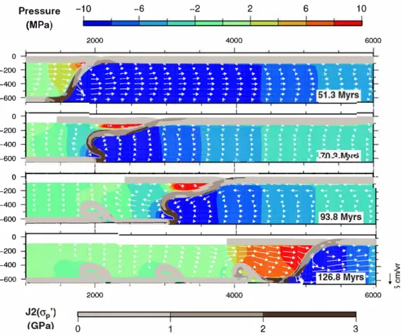
We define a reference experiment with a mantle viscosity of 1 û20Pa .s. The resulting evolution in time is

shown in Figure 9, which displays plates geometry and deviatoric stress 12( eï'p), together with the velocity

and dynamic pressure fields within the mantle.

Folds form successively through time. During this periodic folding, note that the dip of the subducting plate varies at shallow-depth depending on the stage of fold development As a fold forms, the slab dip

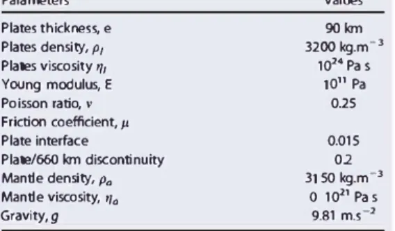
Table 2. Mechanical Parameters for the Subduction Model in Section 5 Parameters Plates thickness, e Plates density, p1 Plates viscosity ,,, Young modulus, E Poisson ratio, v Friction coefficient,µ Plate interface Plate/660 km discontinuity Mande density, Po Mande viscosity, ,,0 Gravity, g Values 90km 3200 kg.m-3 1024 _Pas 1011 _Pa 0.25 0.015 02 31 50 kg.m-3 o 1021 _{Pa s} 9.81 m.s-2

decreases and moves close to the base of the over­

riding plate. When the fold ends, the dip of the slab

increases back to a maximum of nearly 60

0

_.

The velocity field in the fluid also changes during

fold development The upper image shows a rela­

tively unidirectional velocity field that follows the

direction of the slab roll back. Then, with the begin­

ning of fold formation, the velocity field ahead of

the subducted plate moves forward (leftward).

Below this subducting plate, there is a 'circulation

zone," but the magnitude of velocities remains low.

The last figure represents the stage at which the

recently formed fold entrains the fluid down with its

deposition. ln this last stage, the magnitude of velocities regains that of subduction (or the reference veloc­

ity). This fourth image is similar to the first stage (slab rollback). Note that during fold development, in the

mantle, a large zone of relatively high dynamic pressure develops in between the overriding plate and the

flattening slab. Yet with the present mantle viscosity, pressure never exceeds 10 MPa. On the other hand,

within a plate, high deviatoric stresses (> 1 GPa) occur in its most bent parts. Values greater than 2 GPa are

achieved from about 400 to 660 km depth within the bottom fold on the transition zone. These high values

of 1

2

(eï'

_p

) within the plate are not induced by the mantle flow nor drag but by its own folding.

The next numerical experiments aim at studying the effect of varying mantle viscosity with respect to the

reference experiment above as well as with an experiment with an inviscid mantle. Figure 10 displays five

cases with different mantle viscosities after 126.8 Myr of subduction. We represent the final geometries of

plates, and their intermediate geometries are displayed with black lines for different times. Two independ­

ent col or scales are used to describe the second invariant of the deviatoric stresses in the plates

12

(

eï'

_p

) and

in the mantle

12

( eï'

m).

Figure 10 (top) displays the result without a viscous mantle (as in

Gibert et al.

(2012)). Experiments with

mantle viscosities lower than 10

20

_{Pa s do not show any effect on the period nor on the size of slab folds. A}

shift in time (and space) of the formation of the first fold is detected at best. Mant

l

e viscosity needs to be

greater than 1û20Pa .s in order to generate an increase in the folding period (Figure 1 Ob). For mantle viscos­

ities up to s.ox1û20Pa .s (Figures 1 Oc and 1 0d), the folds' width and height both increase with increasing

viscosity, because the viscous fluid under the fold prevents the plate from falling and folding. As a conse­

quence, the time spent in folding is longer. Comparing Figure 1 0a with Figure 1 0d, we note that du ring

folding, the amplitude of the curved part of the subducted plate is greater, thus the resulting fold is bigger.

Both cases in Figures 1 0a and 1 0d display a stage at which the subducting plate adopts a horizontal increas­

ing shape in between 100 and 200 km depth. Actually, this behavior occurs for ail viscosities lower than

s.ox1û20Pa .s.

For greater viscosities (8.0X 1 a2°Pa .s and 10

21

_{Pa .s, Figures 1 0e and 1 Of), we denote a change in the regime}

of fold formation. Fluid escape under the subducting plate becomes difficult. Thus, fold deposition is slower

and bumps form. These "bumps" rise to nearly 250 km of depth, which seems unrealistic (no tomography

has reported such a geometry). Furthermore, the slab cannot flatten in the upper 200 km depth, because

material between the overriding plate and the top of the subducting plate is too viscous.

The

12( a'p)

stress field in the mantle increases in magnitude with increasing mantle viscosity. Wh ile, for a

mantle viscosity of 1 û20Pa .s, the deviatoric stress never exceeds 10 MPa (d., Figure 9), for a larger viscosity

of 1 a2

1

_{Pa .s it is at least twice (Figure 1 Of).}

On the other hand, maximum values of

12

(

eï'

_p

) in plates are not proportional to an increase in mantle viscos­

ity. For low mantle viscosities, more than 2 GPa are achieved within the fold hinges below 400 km depth

(Figures 1 0b-1 0d). ln contrast for high mantle viscosities (::::: 8.0X 10

20

_{Pa .s), slab deposition occurs with lit­}

tle curvature, e.g., the plate is Jess bent and consequently

l2

(eï'

_p

) rarely exceeds 1 GPa.

Other numerical studies that account for a self-consistent temperature-dependent viscosity consider a

lower or similar max

i

mum slab strength (1 GPa) [e.g.,

CizkovéI et al.,

2002;

Bilien,

2010), which sets a lower

Pressure -10 (MPa) 2000 0

•

..

..

--+

--::î

-600

j

-

--•

►

...

..

_•

-2�

j

-₄₀₀ 1 -600 ----...----,

-6

..

•

-

---

---

--

-+

.

.

►

-2

,.

•

.

.

_. -+ -+

..

-

-

-

---

- -

--

-

-+

--

-+ ➔ V ►

.

.

.

► ►

.

►

.

.

► ►

.

.

►

•

> >

2

6 10 4000 6000

.

_{♦ ♦}

-

.

•

..

.

•

V

.

◄

.

•

•

.

•

_►

.

:

1

-+ -+ ➔ ➔

..

+

..

-

-

-

-+ -+ ➔ ♦

-

-

-+ -+ ➔ ♦ -+

..

► ,J

.

_.

.

►

.

► ►

.

►

•

► ► ► ►

.

.

► ►

•

0

--r---... --...._ _ ___._ __

....__

-==

====-

... __ ...._ _ ____. __

"1---200 -400 -600 -.----�--�--�--� -2�

j

-4001 -600

•i-,

--

-

---

---

i

-

-

�

-

---

,

..-

-

-

-

-

--

-

-·

...;;.

....::.

:;:m

�-2000 6000 0

2

3

Figure 9. Reference model with a mantle viscosity of 1Cl20Pa .s. Geometry of plates, second invariant of the deviatoric stresses in the plates,

dynamic pressure and velocity fields in the mantle at different stages.

li mit to the upholding of the slab's coherency. Laboratory experiments on olivine samples produce similar values for temperatures around 10000_{( and high pressure [Weidner et al., 2001), while others obtained plas­} tic yielding above 2.5 GPa [Schubnel et al., 2013). Our modeled slabs exceed 2 GPa rather locally in the sharp bends of folds at 400-660 km depth, which gives us confidence that the slab's mechanical coherency is pre­ served (even though brittle failure and nonlinear flow mechanisms obviously occur during slab folding). And if the slab does 'break' completely, the remnant upper part of the slab will still pile up over its previ­ ously deposited slice, leading to a similar geometry at the large scale. A future step of our study is obviously to account for more complex and self-consistent rheology.

5.3. Effect on Slab Dip and Overriding Plate Stress Regime

Figure 11 a shows temporal variations in the slab dip angle averaged between depths of 100 and 160 km. The 'folding period: corresponding to the time-span between two lowest slab dips, is close to 20 Myr for

l'/a ::; 1020_{Pa .s and reaches 30 and 40 Myr if l'/a 3.0Xl 020and 5.0X10}20_{Pa .s, respectively. Slab dip ampli­}

tudes span a range from about 5° _{to 45}°_{, oscillating Jess with increasing mantle viscosity. The minimum dip}

attained by the slab also reduces with increasing mantle viscosity. This minimum value actually corresponds to a very fiat slab extending over a length of nearly 500 km at about 150 km depth (see the geometry evolution of the top of the subducted plates in Figure 10). Note also that this depth may be reduced if one uses thinner viscoelastic plates (here we assumed 90 km; Table 2). These numbers compare with observa­ tions of the present-clay fiat slab in Central Chi le, extending for about 350 km eastward at about 110 km depth [Marot et al., 2013).

Figure 11 b shows that the far-field horizontal stress of the overriding plate changes also depending on mantle viscosity. Positive values correspond to a tensile regime while negative values correspond to a

1

16 ë 2 12 8

.. --

i

4 0 0

Figure 1 O. Geometries and second invariant of the deviatoric stresses (after 126.8 Myr) for models with different mantle viscosities. Two color scales are used for the stresses in the plates (gray scale to the left) and for those in the viscous mantle (blue to red scale to the right). The black lines show the shape of the top surface of the subducted plate at different times.

compressional regime. With a mantle viscosity of 1 û20Pa .s, tensile and compressional periods alternate, sim­

ilar to the inviscid case shown by Gibert et al. [2012). With mantle viscosities equal to 3.0X 1 a2°_{Pa .s and}

higher, the state of stress remains always compressional. Yet variations of about 100 MPa occur in ail cases, which should still produce significant variations in tectonic structures.

Comparing the temporal evolution of the horizontal stress and the slab dip in Figure 11, we note that the slab dip that corresponds to the transition between compressional and tensile regimes is located a round 40°_{. This value is in agreement with the conclusions drawn from the statistical study by Lallemand et al.}

[2005).

5.4. A Mantle With Two Viscosity-Layers

Rheological studies showed that the viscosity in the mantle varies with depth due to mineralogical phase transfonnations (olivine, spinel, wadsleyite, ringwoodite [e.g., Karato and Wu, 1993)) including the 660 km depth transition zone which constitutes a major jump in viscosity and density. However, it is not clear whether this jump is sharp or progressive, and it seems to vary worldwide. The results described above were obtained with an isoviscous upper mantle. We now perform numerical experiments in which the upper mantle is divided into two layers above and below 200 km depth, according to the approximate limit of low seismic shear waves (also called the Lehmann discontinuity zone).

Results are displayed in Figures 12. The weak upper mantle layer is assigned a viscosity of 1.0Xl û20Pa .s in the cases of Figures 12a and 12b. The more viscous layer underneath is assigned a viscosity equal to S.0X 1 û20Pa .s (Figure 12a) and 1.0X 1 a21 Pa .s (Figure 12b). A third case is presented in Figure 12c, in which the

viscosity of the weak layer is set to 1.0X 1019_{Pa .s whereas the layer below has a viscosity of 1.0X 1 a2}1 _{Pa .s.}

Figures 12b and 1 0d show a strong similarity, indicating that the viscosity directly under the overriding plate plays a first-order role in the formation of folds. Whereas in the isoviscous case, the fluid between the