To cite this version : Desert, Thibault and Authié, Thierry and Trilles,
Sébastien Modelling of the ionosphere by neural network for equatorial
SBAS. (2015) In: ION GNSS+ 2015, 14 September 2015 - 18
September 2015 (Tempa, United States).
O
pen
A
rchive
T
OULOUSE
A
rchive
O
uverte (
OATAO
)
OATAO is an open access repository that collects the work of Toulouse researchers and
makes it freely available over the web where possible.
This is an author-deposited version published in :
http://oatao.univ-toulouse.fr/
Eprints ID : 14320
Any correspondance concerning this service should be sent to the repository
administrator:
[email protected]
Modelling of the ionosphere by neural network
for equatorial SBAS
T. Désert, T. Authié, S. Trilles, Thales Alenia Space, Toulouse, France
1. BIOGRAPHIES
Thibault Désert is currently a Thales Alenia Space
trainee. Soon to be an engineer, he will be graduating from INSA (Institut National des Sciences Appliquées) in June 2015, with a major in mathematical engineering and modeling.
Thierry Authié graduated from the Institut National des
Sciences Appliquées (INSA), France. He worked in space flight dynamics and precise orbit determination. He currently works as navigation algorithms engineer at Thales Alenia Space on the EGNOS project.
Sébastien Trilles holds a PhD in Mathematics (topology
and real algebraic geometry) from the Paul Sabatier University and a post-master graduation in space engineering at the École Nationale Supérieure d’Aéronautique (ISAE-SUPAERO), France. He is a specialist in Navigation Performances, working at Thales Alenia Space on the EGNOS Project as Algorithm Navigation Design Authority.
2. ABSTRACT
The estimation of the ionosphere delay and associated confidence interval constitutes the major issue to reach APV1 availability performance level for single frequency SBAS above the equatorial area.
The ionosphere is a complex physical system which dynamics is particularly disturbed at the Geomagnetic Equator while mid-latitude regions are quieter. Classical methods to compute ionosphere delays, such as those implemented in EGNOS and the WAAS, are specific to a smooth ionosphere behavior and are not really adapted to follow high spatial and temporal gradients, such as those observed in the equatorial area. Thus innovative methods, having flexible and reactivity qualities, shall be defined and adapted to propose efficient equatorial SBAS. Classically in SBAS concept, the knowledge of the ionosphere delay is obtained by a set of lines-of-sight between the network of ground stations and the navigation satellite constellation. Each line of sight intersects the ionosphere layer, assumed infinitely thin, and the dual-frequency combination allows to compute, at
first order, the ionosphere delay that affects the GNSS measurements.
From this set of heterogeneous information, locally sampled irregularly on the sphere and changing over time, we propose to build an interpolating method to calculate the ionosphere delay on a point of interest by an adaptive mesh, unlike fixed grids usually used.
In this paper, we introduce an interpolation method based on the definition of a flexible network that can adapt to the spatial location of the data. It is therefore proposed to create self-organizing maps – as the Kohonen map – defined by a mesh that fits the data. This network ends up sticking to the data by "learning" in real time: the mesh becomes denser and denser in the presence of many measurements and relaxes otherwise. This technique increases the granularity of the ionosphere delay information to compute, in particular to be able to describe the local plasma bubbles or depletions, if they are observable.
The adaptive array technology "learning" has been widely studied in the field of modeling neural networks. Their main advantage is to be able to reach an optimal state based on the information they process. The experimentation based on this technique shows a very good behavior in the case of strongly disturbed ionosphere conditions and the preliminary results are promising to bring the expected robustness to deploy SBAS in equatorial area.
3. INTRODUCTION
The upper layers of Earth's atmosphere, which constitute the ionosphere, perturb the propagation of GNSS signals [5], [6]. These disturbances degrade the accuracy of the distance measurements performed by GNSS receivers, and thus the user location. Besides the diffraction effects, the ionosphere changes the propagation of GNSS signals. Indeed the carrier wave and its modulation (codes) travel at different effective velocities. The code propagation effective velocity decreases and becomes slightly lower than the speed of light, resulting in a delay in distance measurement. The ionosphere delay depends essentially on the signal frequency and density of free electrons in the ionosphere. To address this degradation, SBAS broadcasts to the aviation user ionospheric correction
parameters and integrity data improving the position computation.
The SBAS Minimum Operational Performance Standard document (MOPS, [4]) specifies the way the augmentation data should be transmitted to the aviation users. This document specifies that the ionosphere shall be considered as a thin layer, located at 350 km altitude in the WGS reference frame. Consequently all ionosphere effects are assumed to be concentrated and applied on a single point, the Ionospheric Pierce Point (IPP) defined as the intersection between the thin layer and the line of sight that connects the aviation user and the GNSS satellite.
The MOPS also specifies a discretization of the ionosphere layer by a regular square grid (5 deg per 5 deg except around the pole areas) whose vertices are called Ionosphere Grid Point (IGP). The Message Type 26 of [4] contains the Grid Ionospheric Vertical Delay (GIVD) and the Grid Ionospheric Vertical Error (GIVE, a 1.10-7 confidence interval) on each IGP defined and identified by the Message Type 18 of [4].
Finally the MOPS defines a mapping function, that converts the vertical ionosphere delay into a slant one, and an interpolation method that allows aviation users to compute the ionosphere delay along the line of sight at the IPP from the surrounding IGPs.
In the SBAS context, the ionosphere correction message (MT26) is the one that has the most impact on the system performance, mainly user availability, for single frequency service levels. Consequently the development of an equatorial SBAS faces several difficulties that come from the ionosphere modeling capability. The equatorial area faces strong ionosphere dynamics, such as large spatial and temporal gradients, scintillation effects [7], local plasma bubble [9], [10]. So the challenge is to define a suitable ionosphere model able to track such gradient events so as to fit the TEC field observed through the measurements and to minimize the GIVD error. For equatorial SBAS, other issues can arise by applying the MOPS computation at user level. First the MOPS bilinear interpolation function can introduce an error in the computation of the User Ionospheric Vertical Delay (UIVD) at each IPP. This error increases in case of high non-linear ionosphere dynamics (common above the equatorial area) and is amplified due to the large scale of the IGP distribution. However the SBAS has to protect the user against this error such that the User Ionospheric Vertical Error (UIVE), resulting from the interpolation of four GIVE associated to the surrounding IGP, shall contain the error between the real vertical delay and the one rebuilt using bilinear interpolation. Second the mapping function can produce errors in the estimation of the User Ionospheric Slant Delay (UISD) along the line of sight mainly at low elevation. Nevertheless these questions are not discussed here, the purpose is focused on the minimization of the GIVD error by using adaptive map.
4. PROBLEM CHARACTERIZATION
The characteristic scale depends on the ionosphere conditions (geomagnetic storms or quiet periods). At low latitudes the ionosphere presents a global dynamics with, for the area of interest (i.e. the equatorial area), spatial gradients of the order of 30-50 TECU over 1000 km of distance [8] (1 TECU can be seen as a 16 cm delay for the L1 signal). Thus, changes in gradients of less than 1000 km distances are common features of the ionosphere at these latitudes.
Another physical phenomenon that affects the ionosphere behavior above the equatorial areas are the plasma bubbles. A plasma bubble is a strong electron density contrast area, starting from the lower part of the ionosphere and rising in altitude (high level of ionosphere), and follows the magnetic field lines in the North West direction [9]. The magnetic field strongly controls the generation and behavior of bubbles. In Africa, the magnetic field is smoother than on the South American sector (South Atlantic Anomaly), but the plasma bubbles are more common there, a phenomenon that is not yet fully explained [10].
Finally scintillation effects cause amplitude fading on code phase measurements (10dB observed above Kourou’s station [15]) and phase jitter on the carrier phase measurements. The effect of scintillation on the carrier phase can generate cycle slips and potentially a loss of lock. Scintillations are small-scale plasma irregularities that compose the ionosphere, which translate into a rapid change in the refractive index for the radio signals [7]. Plasma bubbles are at the origin of the scintillation to lower latitudes. Around equatorial area, scintillation is a nocturnal phenomenon that occurs in the first part of the night.
5. STATE OF THE ART ON ESTIMATION TECHNIQUES
Let us consider first the methods used in EGNOS and the WAAS for a short description.
The EGNOS system uses an approximation of the ionosphere thin layer, by a polyhedron which facets are triangles (Triangular Interpolation, TRIN). The technique has been developed by Mannucci and presented in [1]. Each vertex of the TRIN mesh has a constant solar local time and computes the vertical ionosphere delay with a Kalman filter. After computing the vertical TEC (Total Electron Content) on the nodes of the TRIN, the GIVD are deduced by a second triangular interpolation (see [3] for a detailed description). The advantages are first to keep a ionosphere history and second to avoid the Kalman filter following high dynamic night-and-day transition. The limitation of the TRIN is that the method assumes that the ionosphere evolves linearly over a facet. In [2]
some new ideas have been developed to propose an adaptive TRIN mesh. In this context the algorithm creates additional TRIN nodes around a detected local gradient and removes it when normal conditions are recovered. The WAAS has implemented a Kriging estimation, that belongs to the class of geostatistical interpolators [11]. This interpolation provides the best unbiased estimator - in the sense of minimal variance - of the variable to interpolate using linear combinations of neighboring values. In this method, the variable is assumed to be composed of a deterministic part and a random part that is not a Gaussian white noise process, but contains a spatial dependency structure. The advantages are first to solve the GIVD in a single iteration and minimize the number of interpolation operations, and second to provide a method that reduces the GIVE without impacting integrity. One limitation of Kriging is that the method assumes a spatial isotropy of the data. To cope with this difficulty the algorithm may be more complex by defining two variograms, one according to the latitude and the other according to the longitude.
Other techniques exist and are widely used for modeling the ionosphere layer. The spherical harmonics decomposition is a well-known technique to model a thin ionosphere layer. The accuracy of the model depends on the order of the decomposition, and the resolution with high order level depends on the quantity of observables. This approach is efficient for middle latitude areas where the ionosphere behavior is quite smooth. The GIVD computation is given directly by the analytic value of the model at each IGP location.
A Taylor approximation consists in modeling locally the thin ionosphere layer by a polynomial (of degree two classically). The polynomial coefficients are fit using the vertical TEC at IPPs. This technique can be used to compute directly the GIVD on each IGP by adjusting a parabola above each IGP. In this context, the GIVD is identified as the zeroth order coefficient of the polynomial.
Finally, another technique can be developed coming from the image processing and signal reconstruction field [3]. The Adaptive Normalized Convolution method can be viewed as a Local Weighted Mean Least Square; the weighting kernel is given by a local gradient estimation. First the method determines the gradient of samples inside a local ball of a Gaussian filter around the desired point to interpolate (IGP). Second the method deforms the base of the filter in the direction of the lowest gradient in order to interpolate among values evolving slowly. The method is designed to restitute the contour of a rapid change in the data. It is also a direct IGP interpolation from data measurements taking into account the anisotropy of the data.
In middle latitude areas (in particular in the ECAC area, European Civil Aviation Conference) all methods provide
good results and no interpolation method is found to be significantly better than the other (see [3]). In particular there is no specific and local geographic pattern where one method provides better results in term of accuracy. The context of the equatorial area is very different due to rapid changes in the ionosphere dynamics. Some physical events, as plasma bubbles, may appear in regions not observed by measurements, leading wide-averaging techniques to produce GIVD errors that may not be covered by the GIVE. These considerations led TAS to study adaptive mesh, which vertices remain close to the data each time.
6. THEORETICAL DESCRIPTION OF SELF ORGANIZING MAPS
The idea of having an adaptive mesh is to have its nodes constantly moving according to the inputs, in our case the Ionospheric Pierce Points. This way, the mesh is refined in regions where IPP density is high, and looser in the regions where density is lower. This allows having a much finer spatial definition where there is more information. The approach we used to create an adaptive mesh is to use Self Organizing Maps (SOM).
Self-Organizing Maps have been introduced by T. Kohonen in [12], and are a kind of artificial neural network. Artificial neural networks create nonlinear mapping between inputs and outputs. They are made of a set of units, or neurons, who are given a weight (a scalar or a vector). With a series of inputs and associated outputs, they “learn” how to map the two by readjusting their weights. Artificial neural networks can be divided in two kinds: with supervised learning, in which the network must first be “taught” with a training set of input/outputs before it is able to tackle real problems, and unsupervised learning, in which the neural network adapts itself continually without supervision. The Self Organizing Maps belong to the latter.
More precisely, the Self Organizing Maps are made of a set of neurons with connections between one another, thus forming a mesh (fig. 1).
Each neuron is assigned a weight, also called a synaptic vector, which dimension is the same as the inputs.
Figure 1: Representation of a Self-Organizing Map neurons forming a rectangular mesh
When an input data occurs, a competitive learning phase is performed, in which the neuron most similar to the input point is searched. The similarity criterion is usually defined as the Euclidean distance between the input point and the synaptic vector. The most similar neuron is called the Best Matching Unit (BMU). The neurons synaptic vectors are then updated to match more closely the input point. The update amplitude decreases with the distance between a neuron and the Best Matching Unit, therefore a neighborhood function is defined on the network, and is usually the Euclidean distance between synaptic vectors. The update formula for a synaptic vector is:
← + , −
with wi the synaptic vector of neuron i, I the input data vector, and theta the neighborhood function between neuron i and the best matching unit s. Several kinds of neighboring functions can be defined. In the original version of SOMs, every neuron is updated and the neighboring function decreases exponentially with the distance. Other versions of SOMs work more locally, by updating only the Best Matching Unit and its neighbors, with an update amplitude greater for the BMU than for its neighbors.
With this process iterated over every input data, the Self Organizing Map neurons are updated so that they are more resembling to the input data that were fed to the network. The network is thus deformed to match the input data.
Self-Organizing Maps can thus be seen as a way of interpolating data by mapping a continuous input space to a discrete space made by the network neurons. To each vector in the continuous input space, an interpolated value is defined by the synaptic vector of the Best Matching Unit. The learning phase of the network aims at having the best interpolation possible.
Of course, it is possible to have a more sophisticated interpolation formula with a combination of the Best Matching Unit and its neighbors. The synaptic vector update formula must be adapted to match the interpolation formula. This is the base principle of Continuous Self Organizing Maps [13]. In this version, for each vector in the input space, a set of neurons made of the best matching and some of its neighbors are “activated” and given a weight depending on their distance to the input vector, so that the interpolation is a weighted mean of the surrounding neurons, giving a continuous interpolating function.
We have applied the Self Organizing Maps to the ionosphere estimation problem, by means of an adaptation of the TRIN grid built as a polyhedron that discretizes the thin ionosphere layer.
The construction of this grid starts with one of the five Plato solid, the icosahedron (20 regular triangular facets, 12 nodes), that is discretized by considering a new point
in the middle of each edge and forming new sub triangles (four new in each previous facet). This process leads to a more complex polyhedron, automatically not regular, and provides:
2 + 10 ∙ 4 grid points (node), and 20 ∙ 4 triangular facets. where L is the level of discretisation.
We started from the current TRIN grid, which level is 3. The TRIN vertices will be the neurons of the Self Organizing Map, with the edges defining the neighboring relationship of the neurons.
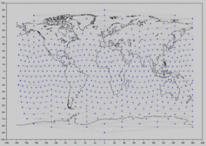
Figure 2 : Original regular mesh over the globe
The synaptic vectors for each neuron is made of the position of the vertices on the sphere. According to the location of the Ionospheric Pierce Points, the synaptic vectors will be updated to look more like the IPP, which means the TRIN vertices will be moved to fit the IPP distribution. It is then expected that the TRIN nodes will be more concentrated where the IPP density is high, giving a better spatial resolution in the TEC estimation. The nodes will conversely be more spaced where the IPP are rare, but since there is much less information in these regions, a reliable finer spatial resolution cannot be obtained anyway.
As for the TEC value estimation, two options are possible:
1. The TEC value is part of the synaptic vector and is estimated using the same learning phase as for the node locations on the sphere.
There are many different adaptation formulas for , , that make sense, we tested many of them and the best one according to GIVD accuracy for our type of data is the following:
, = | | ! < 2
With *% being the distance between the neuron and the IPP , and +)) is the estimation of the error at {-.//, 0.//, 1.//} : the difference between the input 3+4.// and the interpolation. The variability of the data is included with ! being the standard deviation to reduce the impact of an error in case of a great variability.
2. The TEC value is not part of the synaptic vector, and is estimated another way. In our case, it is estimated with a Kalman filter just as with a static mesh.
The one used in EGNOS considers the state of the synaptic weights 5678= 56 and the covariance matrix 9678= 96+ :6 with :6 being the process noise matrix. In this case, since the mesh is time-evolving, we have to update the node synaptic values by interpolating them.
; 96785678= <9= <56< + :6 6
With A being the matrix that has in each line, the weights of the different nodes of the mesh for interpolating the TEC value at its new position. The synaptic vector only contains nodes positions.
Both methods have been tested. A high level analysis of each method is given below.
For method 1, the TEC is treated in the same way as the node locations, the Self Organizing Map learns the IPP distribution along with the IPP TEC values. All of it is done with the same process and does not require an additional method to estimate the TEC values. However, in this problem, we deal with uncertainties in the input data, which come from measurements flawed with errors. Also, an SBAS needs to provide users with a confidence interval (GIVE) on the TEC value estimated on the IGP. It is therefore necessary to have a measure of the estimation quality. This is the main weakness of the Self Organizing Maps, as there is no clear way to process the input variances in the learning phase, nor to have an estimation variance after the learning phase has updated the synaptic vectors. Several attempts have been made to deal with such problems, giving another unsupervised training neural networks, called the Generative Topographic Mapping (GTM) [14]. However, even with GTM, dealing with input data variances is not straightforward, and still does not give an output estimation variance. This method shall be called “SOM” below.
For method 2, two processes need to be implemented and interlaced. The learning phase of the SOM moves the TRIN nodes on the sphere, and then an iteration of the Kalman filter is performed to estimate the TEC value on the TRIN nodes. Of course, the propagation step of the Kalman filter must take into account the node displacements. That being said, the Kalman filter allows
taking the IPP TEC variances into account in a straightforward way, and also provides an output TEC variance. This allows the TEC estimation to be optimal in the sense of the Kalman filter optimality properties, thus minimizing the GIVD error. This method shall be called “Adaptive Kalman” below.
7. RESULTS AND DISCUSSION
As the concerns of this study is the equatorial zone, the experimentations have been made above the geographic zone delimited by [-10 deg, +30 deg] in latitude and [-25 deg, +30 deg] in longitude that corresponds to ASECNA service area (air navigation African agency).
The results have been obtained using the data coming from both the SAGAIE network and IGS stations located inside the ASECNA area.
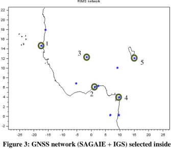
The SAGAIE network is a set of GNSS stations that cover the West African Region [15]. The stations currently deployed are all installed on major airports of the ASECNA area: Dakar (1), Lomé (2), Ouagadougou (3), Douala (4), N’Djamena (5).
The network considered for the experimentation is presented in figure 3.
Figure 3: GNSS network (SAGAIE + IGS) selected inside ASECNA area
During the experimentation, the methods SOM and Adaptive Kalman have been tested to try to improve the ionosphere estimation already implemented. Every method implemented relied on the same adaptive mesh fitting the distribution of the IPP.
To illustrate the tailoring, the mesh over the equatorial ASECNA zone is presented in Figure 4. We injected 36 hours of sample data in our algorithms and the red points represent the IPP at the last period of time.
1
2 3
4 5
Figure 4 : Mesh (in blue) adapted to 36h of input data, and IPP (in red) at a given date
Compared to the original mesh on Figure 2, there are more nodes on the equatorial part, implying that the triangles are wider in other areas.
The challenge regarding the adaptive mesh is to define a node displacement tuning able to ensure the stability of the mesh all the time. In other words, the move of all nodes shall be controlled to avoid degeneracy of the triangles along time. The tuning presented here preserves the global shape of the initial TRIN, the triangles are only stretched or tightened so that the global geometric properties (isosceles, equilateral) are kept.
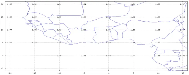
In order to compare our maps to a reference, EGNOS RMS map –the Root Mean Square of the error between the estimate and the truth data- is presented on Figure 6. However, EGNOS IGP are not monitored during the whole of the day. The monitoring proportion goes from 3% to 100% for one IGP on the area we study. Therefore, the maps generated with our methods and presented below are only considering the error at the EGNOS monitoring time.
Using the adaptive mesh, the Self Organizing Maps method is analysed first. Figure 7 shows the RMS map over the equatorial IGP on ASECNA using method 1. The SOM adaptation provides a really good fit to the input data as long as there are enough measurements with a small variability. However, several IGP are poorly estimated at some points in the area with a great variability. Since the variability of input data cannot be taken into account in the SOM adaptation, the Kalman filter seemed a better way to estimate the TEC.
The Kalman filter offers a strength regarding the variability of the data, recognizing the significance of an IPP compared to the past ones for the TEC fitting. Moreover, the Kalman formulation has a self-management of measurement noise and provides automatically a formal covariance for all elements of the state vector. It is thus possible to associate a confidence level for each measurement during the process of the TEC computation. The computation time consumed by the Kalman process is equivalent.
Figure 8 shows the RMS map on ASECNA using the adaptive Kalman filter method.
The results are better than EGNOS using the Adaptive Kalman filter. Indeed, 31 of the 38 IGP on the map are more precisely interpolated on average with the adaptive mesh method. The adaptive mesh method does not provide a GIVE estimation at the moment, so the results are compared to EGNOS GIVD values on EGNOS monitoring period.
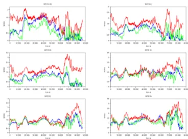
In order to compare the GIVD error evolution during the whole period, we pick the 6 most monitored IGPs (between 94% and 100% of monitoring time) and display each method results. Figure 5 shows the GIVD error evolution of EGNOS (red), the SOM (blue) and the Adaptive Kalman filter (green).
Figure 5 : GIVD error evolution on the 6 most monitored IGP
Below is a table with the GIVD error RMS for these IGP, with the three methods:
IGP(10,10) IGP(10,5) IGP(10,0)
EGNOS 1.35 m 1.57 m 1.80 m
SOM 0.94 m 0.92 m 1.02 m
Adaptive Kalman 0.75 m 0.86 m 0.91 m
IGP(5,10) IGP(5,5) IGP(5,0)
EGNOS 1.67 m 1.66 m 1.63 m
SOM 1.38 m 1.39 m 1.30 m
Adaptive Kalman 1.33 m 1.32 m 1.23 m
Overall GIVD error values are lower than the ones produced by EGNOS, the TEC is more precisely fit. In particular for IGP (lat 10 deg, long 10 deg) and (lat 10 deg, long 5 deg), during the night, when the scintillation effects are particularly strong, the GIVD error are much improved.
Figure 6 : EGNOS RMS map
Figure 7 : SOM RMS map
8. CONCLUSIONS AND PERSPECTIVES
Two TEC tailoring methods have been implemented and tested. Both based on adaptive mapping, they provide better GIVD error RMS than the method implemented in EGNOS. First, the Self Organizing Map using an exponential function practically always provides a very good fit to the input data. Nevertheless, GIVD error spikes can occasionally occur on a few IGP when input measurements are very noisy.
In order to take into account the error inherent to a measurement, an adaptive Kalman filter is best suited for the task. This second method also provides better GIVD errors than EGNOS and avoid GIVD error spikes thanks to its capacity to deal with the covariance contrarily to the SOM method.
Therefore a new method to improve GIVD accuracy is proposed. The accuracy improvement allows to reduce the GIVE while maintaining the same integrity margins hence improving availability. It is shown that this method is effective on an equatorial region. These results support the idea that equatorial SBAS is possible.
9. ACKNOWLEDGMENTS
The authors would like to thank Michel Monnerat at TAS, Hugues Secretan at CNES and Roland Kameni at ASECNA for the availability of SAGAIE data used for the experimentations.
10. REFERENCES
[1] A.J. MANNUCCI, B.D. WILSON, C.D. EDWARDS, A new method for monitoring the
Earth’s Ionospheric Total Electron Content Using the GPS Global Network, ION GPS 1993
[2] S. TRILLES, G. de la HAUTIERE, M. van den BOSSCHE, Adaptative ionospheric electron
content estimation method, ION GPS 2012
[3] P. ALLEAU, G. BUSCARLET, S. TRILLES, M. van den BOSSCHE, Comparative Ionosphere
Electron Content Estimation Method in SBAS Performances, ION GPS 2013
[4] Minimum operational performance standards for Global positioning system / wide area
augmentation system airborne equipment,
DO-229D rev 1, Jan. 2013, RTCA ed. Washington, DC.
[5] J.L. GOODMAN, Space Weather & Telecommunications, The Kluwer international
series in engineering and computer science, Springer 2005
[6] B. ARBESSER-RASTBURG, N. JAKOWSKI,
Effects on satellite navigation, Space Weather-
Physics and Effects, Springer 2007
[7] P.M. KINTNER, B.M. LEDVINA, E.R. de PAULA GPS and ionospheric scintillations, Space Weather 2007, 5, S09003
[8] K. HOCKE, K. SCHLEGLE, A review of
atmospheric gravity waves and travelling ionospheric disturbances: 1982-1995, Annales
Geophysicae, 1996, 14 (9), 917–940
[9] M.C. KELLEY, J.J MAKELA, O. de la BEAUJARDIERE, J. RETTERE, Convective
ionospheric storms: A review, Geophys. 2011,
49(2)
[10]C.S. HUANG, O. de la BEAUJARDIERE, P.A RODDY, D.E. HUNTON, J.Y LIU, S.P CHEN,
Occurrence probability and amplitude of equatorial ionospheric irregularities associated with plasma bubbles during low and moderate solar activities (2008–2012), J. Geophys. Res.
Space Physics, 2014, 119, 1186–1199
[11]J. BLANCH, An Ionosphere Estimation Algorithm for WAAS Based on Kriging, ION
GPS 2002
[12]T. KOHONEN, Self-organized formation of
topologically correct feature maps. Biological
Cybernetics, 1982, 43:59-69
[13]M. AUPETIT, P. COUTURIER, P.
MASSOTTE, Function Approximation with
Continuous Self-Organizing Maps using Neighboring Influence Interpolation, Proc. of
Neural Computation, 2000
[14]K. KIVILUOTO, E. OJA, S-Map: A network
with a simple self-organization algorithm for generative topographic mappings, Advances in
Neural Information Processing Systems, 1998 [15]H. SECRETAN, S. ROUGERIE, L. RIES, M.
MONNERAT, J. GIRAUD, R. KAMENI,
SAGAIE: A Network of GNSS station to investigate the ionosphere behaviour in sub-Saharan regions, InsideGNSS, Oct/Nov 2014