Cutter-workpiece engagement calculation in 3-axis ball end milling considering cutter runout

Open Archive Toulouse Archive Ouverte (OATAO)

OATAO is an open access repository that collects the work of some Toulouse

researchers and makes it freely available over the web where possible.

This is

an author's

version published in:

https://oatao.univ-toulouse.fr/23731

Official URL :

https://doi.org/10.1016/j.jmapro.2019.03.025

To cite this version :

Any correspondence concerning this service should be sent to the repository administrator:

tech-oatao@listes-diff.inp-toulouse.fr

Sai, Lotfi and Belguith, Rami and Baili, Maher and Dessein, Gilles and Bouzid, Wassila

Cutter-workpiece engagement calculation in 3-axis ball end milling considering cutter runout.

(2019) Journal of Manufacturing Processes, 41. 74-82. ISSN 1526-6125

OATAO

Cutter-workpiece engagement calculation in 3-axis ball end milling

considering cutter runout

Sai Lotfi

a,⁎

_{, Belguith Rami}

a,b

_{, Baili Maher}

b

_{, Dessein Gilles}

b

_{, Bouzid Wassila}

a

a _{Unité de Génie de Production Mécanique et Matériaux, ENIS, Route Soukra Km 3,5-B.P. 1173-3038, Sfax, Tunisia}

b _{Université de Toulouse, INPT/ENIT, Laboratoire Génie de Production, 47 avenue d'Azereix, BP 1629, F-65016, Tarbes Cedex, France}

A R T I C L E I N F O Keywords:

Ball-end milling Runout

Cutter workpiece engagement region Chip thickness

Cutting forces

A B S T R A C T

In order to obtain desired surface quality, the machining parameters such as feed per tooth, spindle speed, axial and radial depth of cut have been selected appropriately by using a process model. The surface quality and the process stability are related to cutting forces which are more influenced by the instantaneous chip thickness and the cutter-workpiece engagement (CWE) region. To reach a high accuracy in cutting forces calculation it is primary to determinate the start and the exit angles on the (CWE) region. Unlike previous studies which cal-culated the (CWE) numerically. This paper proposes an analytical model to calculate the (CWE) region by de-termining the cutting instantaneous flute entry and exit angles. These locations are calculated according to the heights of axial depth of cut. The second proposed approach is to calculate the instantaneous undeformed chip thickness. These solutions are used to calculate accurately the cutting forces in the case of the 3 axis milling operations.

To validate the model, a mechanistic cutting forces model was simulated and compared to the measured one. A good agreement between them was proved.

1. Introduction

The goal of the virtual simulation is to aid the producer to choose the adequate machining parameters before the realization of the parts on the machine tools. These parameters are chosen according to the imposed quality criteria. The most important criterion is the topo-graphy of the machined surface; it is influenced by the flexion and vi-brations phenomena resulting from the cutting forces.

The cutting forces modeling gains more importance in order to prevent excessive cutter deflection and surface errors in milling process. Its prediction is not easy because of the difficulty to control the cutting geometries during machining. In fact, it is important to determinate the instantaneous flute enter and exit angles, this information help to know the exact value of the instantaneous chip thickness and the cutting length which are the two fundamental parameters in the determination of the cutting forces from mechanistic models.

In the previous works, some researchers have been interested in the calculation of the (CWE) region. Ju et al. [1] proposed a discrete boundary representation based on the exact Boolean method to calcu-late the (CWE) at every cutter location. Zhiyang [2] proposed a method based on the tessellated format. The CAD surface model is stored in tessellated format as an STL file which is transformed in a very large

number of triangular facets. The algorithm finds the intersection curves form one or multiple closed regions on the ball end mill which forms the (CWE) regions. Boz et al. [3] compared two models for (CWE) calculations. The first method is a discrete model which uses three-or-thogonal dexelfield and the second method is a solid modeler based model using parasolid boundary representation kernel. The second method was proved more accurate. In the study of Kiswanto et al. [4], the (CWE) region is determined by finding the length of each cut at every engagement angle between the lower engagement (LE) point and the upper engagement (UE) point and the swept envelope of the re-moved volume. Ozturk and Lazoglu [5] proposed a numerical method to determine the chip load of a ball-end mill during free-form ma-chining. The chip load was obtained by defining three engagement boundaries: the tool entry boundary, the exit boundary and the work-piece surface boundary.

Iwabe et al. [6] calculated the chip area of the inclined surface machined by ball end mill cutter by a contour path method using 3D-CAD. The chip area is calculated by the interference of the rake surface and the chip volume. Sato et al. [7] calculated the (CWE) region based on the geometric tool-workpiece intersection in order to predict the topography and surface roughness as a function of cutting parameters. The geometric model is presented in the case of a flat surface machined ⁎_{Corresponding author.}

by a ball end mill on one way strategy. Another phenomenon which influences the (CWE) region and the chip thickness and is not con-sidered in this study is the motion errors of feed drive systems. Then, Nishio et al. [8] investigated the influence of dynamic motion errors of feed drive systems onto the surface machined by a square end mill.

In the study of Erdim et al. [9], the (CWE) is calculated from the output Cutter Location data file by an analytical simulation. Gong et al. [10] determined the (CWE) using a triangle mesh model and the in-tersection calculations of the cutter swept volume. Ozturk et al. [11] and Erdim and Sullivan [12] calculated the (CWE) by subtracting it from the swept volume of tool motion. The tool is divided into ele-mentary disks and the engagement points are extracted, then the start and exit angles are calculated.

Sun et al. [13] calculated the (CWE) using a Z-map model. The workpiece is meshed into small grids whose projection onto the x–y plane is a square. The engaged cutter element can be achieved ac-cording to the difference between the cutter element and the projection of the instantaneous workpiece height into the cutter element.

Boz et al. [14] used a B-rep modeler to calculate the (CWE). In the study of Mamedov and Lazoglu [15] a method based on solid modelers was employed in which the (CWE) was calculated at each cutter loca-tion point. From the cutter localoca-tion file, the swept volume of the tool was calculated and subtracted from a blank workpiece. After subtrac-tion, the start and exit angles of each discretized cutting disc were calculated.

The approximation proposed by Zeroudi et al. [16], calculates the (CWE) as a region delimited by three boundaries. The first was the relative position of the workpiece uncut surfaces. The second was the previous tool path considered without any tool deflection and with perfect surface finishes and has a cylindrical form. The third was the path of the previous tooth considered as a circular path. An analytical model was proposed by Sai et al. [17], where the cutter runout error was neglected.

The (CWE) zone between the tool and the machined part represents the integration limits used in the calculation of the cutting forces. The instantaneous cutting chip thickness can also be modeled correctly by knowing the area of engagement between the part and the tool. The validation of these models requires the modeling of the cutting forces. In the mechanistic method, cutting forces are assumed proportional to

the uncut chip thickness or cutter swept volume.

Yucesan and Altıntaş [18] proposed a ball-end mill forces model based on a mechanistic relationship between cutting forces and chip load. This model discretizes the ball-end mill into a series of disks and describes in fairly rigorous detail the ball-end mill geometry and chip thickness calculation. In the study of Ko and Cho [19] the dynamic effect is considered in the chip thickness model. For more accuracy in the prediction of the cutting forces, Altintas and Lee [20] proposed a mechanistic cutting forces model for 3D ball-end milling using stantaneous cutting forces coefficients. These coefficients are in-dependent of the cutting conditions and are set as a function of the instantaneous uncut chip thickness only. They consider the size effect produced near the tool tip at the low values of undeformed chip thickness.

Liu et al. [26] proposed a theoretical dynamic cutting forces model for ball-end milling using the integrated method. The elementary cut-ting forces components are integrated using the slices elements of the flute along the cutter-axis direction. The size effect of undeformed chip thickness and the influence of the effective rake angle are considered in the formulation of the differential cutting forces based on the theory of oblique cutting.

Cheng [27] studied the influences of tool the wear, the tool breakage and the vibrations in the machining process which increase the cutting forces and causes a poor surface roughness.

In this paper, the models of the instantaneous chip thickness and the (CWE) zone is developed for the calculation of the cutting forces for flat surfaces perpendicular to the tool axis and considering the runout error. The content is presented in the following section as follows: First, the geometrical description of the trajectory of an arbitrary point P in the (CWE) is presented in the local coordinate system attached to the center of the tool then in the local coordinate system attached to the spindle. Second, these coordinates are transformed to the global coordinate system attached to the workpiece. Third, based on the tooth trajectory and the geometry of the milled surface, the cutter workpiece engage-ment (CWE) is analyzed and the entrance and exit angles are extracted, then the instantaneous undeformed chip thickness is calculated. Finally, a simulation using Matlab software was proposed to predict the cutting forces based on a mechanistic approach.

The predicted forces are compared with the measured ones where Nomenclature

P Point in the intersection between the cutter and the workpiece

RW Coordinate system attached to the workpiece

RH Coordinate system attached to the spindle

RC Coordinate system attached to the center of the cutter

e Runout error (mm), offset distance between ZH axis and

ZC axis

ρ The initial eccentricity angle (°), measured at t=0, be-tween YC axis and YH axis

ae Radial depth of cut (mm)

ap Axial depth of cut (mm)

fz Feed per tooth per revolution (mm/tooth/rev)

Pr Plane defined perpendicular to the tool axis ZC, contains

YC and YH axis

Pae Plane perpendicular to the plane Pr, contains cross feed direction and ZCaxis

Pfz Plane perpendicular to the plane Pr, contains feed direc-tion and ZCaxis

z The local height of point P

i0 Tool Helix angle (°)

θ revolution angle (°)

φ(z) Locating angle of point P measured in Pr plane between

OCP and XCaxis (°)

z Local height of point P (mm)

R0 The tool radius (mm)

R(z) The local circumference radius of point P, distance of point P to axis ZC (mm)

ψ The included angle between OCP and ZC axis (°) t The instant time (s)

Vf Feed rate (mm/min)

w Spindle speed (rd/s)

N Spindle speed (rev/min)

Nf Number of teeth

θst Start angle in the cutter-workpiece engagement region (°)

θEx Exit angle in the cutter-workpiece engagement region (°)

tn Instantaneous undeformed chip thickness (mm)

db Infinitesimal chip width (mm)

dS The infinitesimal length of cutting edge (mm)

ktc, krc, kac Tangential, radial and axial cutting force coefficient (N/

mm2)

kte, kre, kae Tangential, radial and axial cutting edge coefficient (N/

mm)

dFt,dFr, dFa The differential cutting forces in tangential, radial and axial direction (N)

2. General formulation of the coordinate system

In this work, a ball nose end milling cutter with two teeth Nf= 2, uniformly distributed was considered, R0is the cutter radius and i0is its helix angle. P (XP, YP, ZP) denotes intersection points between the cutter and the work-piece. The coordinate system is established in order to obtain the parametric equation of the point P in the global coordinate system RWattached to the workpiece.

R OW( W,XW, YW, ZW): The global coordinate system attached to the workpiece in which the tool path is definedFig. 3.

R O XH( H, H, YH, ZH): The local coordinate system attached to the spindle of the mill machine. It moves in the direction of feed rate speed relative to the workpiece. ZHis the axis of the spindle and OHand Oc are in the plane (Pr) perpendicular to the tool axis during milling process, Fig. 1.

R O XC( C, C, Y ZC, C): The local coordinate system fixed on the center of the cutter.

Considering initially at t = 0, that O YH H and the vector of cutter runout, e, are aligned. In this position the initial eccentricity angle measured between O YC C and O YH H is ρ. When the cutter revolves around the spindle axis O ZH Hby a rotate angle θ, the total rotates angle betweenO YC Cand O YH H Become (θ + ρ) as shown inFig. 1.

3. Mathematical description of the trajectory of cutting edge The coordinates of a point P on the ith_{cutting edge in the local} coordinate system R O X Y ZC( C, C, C, C) as are shown inFig. 1 are ex-pressed by the Eq.(1)as (Fig. 2):

= = O P X Y Z R z cos z R z sin z R | ( ) ( ( )) ( ) ( ( )) [1 ] C Rc P P P Rc 0 tan iz ( ) ( )0 (1)

The different parameters φ(z) and R(z) are calculated as follows:

= =

z and R z R z z

( ) ztan i_R0( )0 ( ) 2 0 2

The position of the point P is written in the coordinate system RHas:

= = + O P X Y Z esin ecos M R z cos z R z sin z R | ( ) ( ) 0 ( ) ( ( )) ( ) ( ( )) [1 ] H RH P P P RH R CH z tan i _Rc 0 ( )_{( )} H 0 (2)

Where MCHis the matrix transformation from R O X Y ZC( C, C, C, C)to

R O XH( H, H, YH, ZH). = + + + + M cos sin sin cos ( ) ( ) 0 ( ) ( ) 0 0 0 1 CH

The coordinates of point P in the global coordinate system attached to the workpiece R O XW( W, W, YW, ZW)are expressed by the Eq.(3):

= = + + O P X Y Z X Y Z esin ecos M R z cos z R z sin z R | ( ) ( ) 0 ( ) ( ( )) ( ) ( ( )) [1 ] W RW P P P RW OH OH OH RW R CH z tan i _Rc 0 ( )_{( )} H 0 (3)

Where: XOH, YOHand ZOHare the coordinates of point OHin the global coordinate system RW.

The Eq.(3)can be developed as:

= + + + = + + + = + X X esin R z sin z Y Y ecos R z cos z Z Z R ( ) ( ) ( ( )) ( ) ( ) ( ( )) [1 ] p OH p OH p OH 0 _{tan i}( )_{( )}z_{0 (4)}

In this paper the study considers the one way machining strategy where the feed rate is in X axis direction, the cross feed is in Y axis direction. For these hypotheses the Eq.(4)of the trajectory of point P in the global coordinate system RWcan be written as Eq.(5):

= + + + = + + = X V t esin wt R z sin wt z Y ecos wt R z cos wt z Z R ( ) ( ) ( ( )) ( ) ( ) ( ( )) [1 ] p f p p 0 _{tan i}( )_{( )}z_{0 (5)}

Where t is the instant time and Vfis the feedrate

4. Cutter / workpiece engagement region in ball end milling process

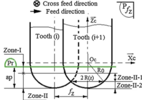
The (CWE) determination is not easy in ball end milling. The en-gagement region for any elementary disc is bounded between the start and exit angles which changes according to the local height of ele-mentary disc.Fig. 3shows the representation of the different (CWE) zones and the planes in a 3D view used in the next step to define dif-ferent geometrical parameters. In ball end milling process, the tooth feed is kept to comparably less than the radial depth of cut. In general the ratio feed/radial depth (fz/ae) is less than one third. The radial depth of cut aeis considered bigger than the feed per tooth fz.

To calculate the entry and the exit angles for any elementary disc, it is necessary to determine the trajectory of the point P, the intersection of this disc and the workpiece. Examining the trajectories of the dif-ferent points P for the (i+1)th _{tool path for each local height z, as} shown in theFig. 4-a. we can distinguish three configurations detailed inFig. 4-b–-d.

The first configuration is when the teeth do not make a complete rotation in contact with the material and exit on surfaces generated by the (i)th_{tool path, this upper part is noted zone-I and its form of} tra-jectory is presented inFig. 4-b. The second is when the teeth make a complete rotation in contact with the workpiece noted zone-II. We distinguish in lower part two configurations that can be noted zone-II-1 and zone-II-2. Their forms of trajectories are presented respectively in

Fig. 4-c and -d. So the (CWE) region can be divided into three zones.

The first is represented in the plane (Pae) defined by the cross feed di-rection and the ZCaxis of the tool, as shown inFig. 5. The second and the third are represented in the plane (Pfz) defined by the feed direction and the ZCaxis of the tool as shown inFig. 6.

Based onFigs. 5 and 6, the zone-I is the region for 2R(z)≥aeand the zone-II is for 2R(z) < ae. The zone-II is then divided into two zones. The zone-II-1 is the region for fz≤2R(z) < aeand the zone-II-2 is for 2R

Fig. 1. Location of point P on the cutting edge view in plane Pr. they present a good agreement.

• • • • • • • • • • • • • • • • • • •

[ l [ _:_]

r:p

✓

•

[ l

[

: l

• • •

[

e

e

p -p

e

e

p p

l

• • • •

[ l

[

l

[

: l

[

(

(

•

[

_:_ l

• • •

-; l

Tool Rotation Center Spindle Rotation Center

e

e

'P

e

P - r:p

e

P - r:p 'P p-r:p p-r:p

"CEl

(z) < fzas is shown in the view in the plane (Pfz). Each zone in the (CWE) region can be identified in ZCaxis direction by its local height z as Eq.(6):

R R a z a for the Zone I R R f z R R a for the Zone II

z R R f for the Zone II

( /2) ( /2) ( /2) 1 0 ( /2) 2 e p z e z 0 02 2 0 02 2 0 02 2 0 02 2 (6)

Fig. 2. Location of point P in coordinate system attached to the tool view in

plane Pae.

Fig. 3. (CWE) region and different planes representation in 3D view.

Fig. 4. Teeth trajectories configurations in three zones, (a): CWE zones, (b): teeth trajectories in zone-I, (c): teeth trajectories in zone-II-1, (d): teeth trajectories in

zone-II-2.

Fig. 5. (CWE) region Zone-I and Zone-II, view in plane Pae.

Fig. 6. (CWE) region Zone-II-1 and Zone-II-2, view in plane Pfz.

Workpiece

- - - -7

(b)

Surface generated

by tool patl1 (i+ 1)

(

-✓

::::;

®

Feed direction

...,_ Cross feed direction

::::;

(i)

th

Path

~

(i+l)

th

,

Path

®

Cross feed direction

_.. Feed direction .

::::; ::::; ::::; ::::;

-✓

~~~=~~ctories (c) Teeth trajectories (d) Teeth trajectories

~dr

Surface generated

by tool path (i)

Surface generated Surface generated

by tool path (i+l) by tool path (i+ 1)

Zone-I

Zone-II

Xc

--Zone-Il-1 Zone-Il-2

= = z cos S z R z z cos a R z ( ) 1 ( ) ( ) , ( ) (1 / ( )) St 1 h1 EX 1 e (7) The calculation of the start angle needs the determination of the distance Sh1.

For determining the exact distance Shk(z), the coordinates of the point Akin the cutter workpiece engagement region must be known first. The start point Akat θStstart angle of the tooth verifies the Eq. (8) of the trajectory. = + + + = + X ( )t V t esin wt( ) R z( ) sin (wt ( ))z (2k 1)f 2 Ak k f k k k z (8-1) = + + YAk( )tk ecos wt( k) R z cos wt( ) ( k ( ))z (8-2)

Where Vfis the feed rate, tkis the instant time, k is the index of the entrance point Ak, the distance Shk(z) at point Akas shown inFig. 8is expressed by Eq.(9):

= = +

Shk( )z R z( ) YAk( )tk R z( )(1 cos (wtk ( )))z ecos wt( k) (9) For the elementary discretized disc with an effective radius R(z), the only unknown in this equation is the instant time tkwhich must be determined through the Eq. (8-1) which can be written as Eq.(10):

+ + + = +

V t esin wt( ) R z( ) sin (wt ( ))z (2k 1)f 2

f k k k z ₍₁₀₎

The determination of the distance Sh1(z) needs the determination of the coordinates of point A0 correspond to the entrance angle θSt as shown in figure, at X(A0)=fz/2 the instant time t0corresponding to this intersection is the solution of the Eq. 11.

+ + + =

V t esin wt( ) R z( ) sin (wt ( ))z f

2

f 0 0 0 z ₍₁₁₎

The solution of this equation t0is subsequently used to determinate the coordinate Y(A0), the distance Sh1(z), the start and exit angles are determined by Eq.(7).

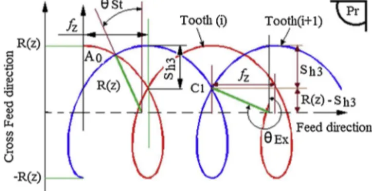
4.2. The engagement Zone-II-1

The trajectory of the point P in the engagement Zone-II-1 is shown

inFig. 9. This zone is characterized by the condition fz≤ 2R(z) < ae.

The start angle is calculated as in the zone-I. The exit angle is calculated when the tooth (i+1) reached the position of point B0. The instant t1is calculated by the resolution of the Eq.(10) for k = 1. The traveled distance by the tooth (i+1) from zero to exit point B0in X direction is X

(t) = 3fz/2. The tooth passes three times by the X coordinates equal to

3fz/2Fig. 9. The point B0corresponds to the second passage at time t1.

When the time t1is known, the distance Sh2is calculated and the exit angle is calculated. The start and exit angles are expressed by the Eq.

(12). = = + z cos S z R z z cos S z R z ( ) 1 ( ) ( ) , ( ) (1 ( )/ ( )) St 1 h1 EX 1 h2 (12) The intersection of the two teeth trajectories is at the point B0as shown inFig. 9, at X(B0) = 3fz/2 the instant time t1corresponding to this intersection is the solution of the Eq.(13)

+ + + =

V t esin wt( ) R z( ) sin (wt ( ))z 3f

2

f1 1 1 z ₍₁₃₎

Fig. 7. Teeth trajectories, start and exit angles in the Zone-I.

Fig. 8. Representation of the distance Shk(z) and entrance point Ak.

Fig. 9. Start and exit angles of the engagement region (Zone –II-1). 4.1. The engagement zone-I

In the plane view (Pr), the distance between the initial and final workpiece curves is the radial depth of cut ae. This region represents the material removed for one pass. The zone-I is the region, where the point

P in the cutting-edge exits on the initial workpiece curve as is shown in

Fig. 7. The produced chip is represented by the A0BC area. The curves

A0B and A0C are two successive teeth trajectories. The points B and C are respectively exit points of the tooth (i) and (i+1) at a distance of instantaneous feed per tooth fz. The entry and exit angles corresponding to (i+1)th _{teeth trajectories are respectively expressed as follows:}

0 fz/2 fz Tooth (i+ 1) ---R(z) YAk

e

_{-( - - ) e}

R(z) _Tooth

_(i

_;

~

x

- - ----•

Feed direction

p- r:p -R(z) p - r:p p- r:p p- r:p

e

_{-( - - ) e}

7r p- r:p p- r:p I:: 0 "J:I u <l)

ae

!

'6

-0 <l) <l) i:...

"'

"'

Initial workpiece cmve

---0

...

u

O

w

---•

Xw

The solution of this equation is next used to determinate the co-ordinate Y(B0), the distance Shk(z) and the exit angle.

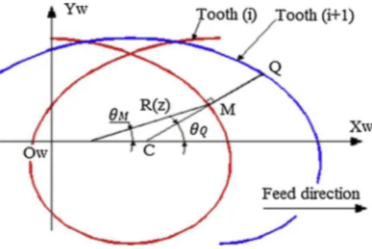
4.3. The engagement zone-II-2

The point P on the (CWE) region Zone-II-2 rotates and does not intersect in the previous cutting tooth trajectory at the exit point as is shown in Fig. 10. The zone II-2 is characterized by the condition (0 ≤ 2R(z) < fz). The start angle is calculated for instant time t0when the tooth (i+1) travels a distance X(t)=fz/2 at point A0as was devel-oped previously. The exit angle is calculated for the instant t2at point

C1when the tooth (i+1) travels a distance equal to 2fz. The instant t2is the solution of the Eq.(14)for the second pass of the tooth (i+1) from point C1.

+ + + =

V tf 2 esin wt( 2) R z( ) sin (wt2 ( ))z 2fz (14) When the instant t2and the distance Sh3are known, the exit angle can be calculated. The entry and exit angles are respectively expressed as follows Eq.(15): = = z cos S z R z z cos S z R z ( ) (1 ( )/ ( )), ( ) 2 (1 ( )/ ( )) St 1 h1 EX 1 h3 (15) In ball end milling process, the (CWE) region varies along the cutter axis. The engagement region is calculated between the lower and the higher elementary discs in contact on the workpiece and for each dis-cretized disc, between the start and exit angle. TheFig. 11shows the variation of the start and the exit angles. For the same immersion depth, the engagement region is larger when the radial depth increases. In the same radial depth of cut, the engagement region increases when the immersion depth decreases.

5. Cutting forces model

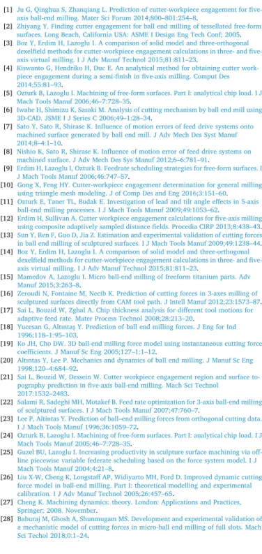
The real tooth motion is trochoidal, resulting from rotational motion of the spindle and the translational motion of the work piece. The calculation of the instantaneous undeformed chip thickness is based on the mathematical relationship between the tooth paths generated by different teeth on one milling cutter. The chip thickness for a tooth engaged in cutting (i+1) is determined through finding the intersection point of the path curve left by the preceding tooth (i) and the line passing throuter axis C, Sai et al. [21] (Fig. 12).

The instantaneous chip thickness tnis calculated for any elementary disc of the cutter. The position in Z direction of the point P between the tooth and the workpiece is constant and the position in XY plane change. To determinate tnit is important to know the distance MQ first. When the tip of the tooth No (i) reaches the position of point M(XM, YM,

ZM) the angular position at instant t1is equal to θM, the location of point

M can be determined from Eq.(16):

= + + + = + + X z V t esin R z Sin z Y z ecos R z Cos z ( , ) ( ) ( ) ( ( )) ( , ) ( ) ( ) ( ( )) M f M M M M M 1 (16) The center of the cutter is located at the position of point C, de-termined from Eq.(17)

= = X z V t Y z ( , ) ( , ) 0 C f C 2 (17) When the tip of the tooth No (i+1) reaches the position of point Q

(XQ, YQ, ZQ) the angular position at instant t2is equal to θQ, the location of point Q can be determined from Eq.(18):

= + + + = + + X z V t esin R z Sin z Y z ecos R z Cos z ( , ) ( ) ( ) ( ( )) ( , ) ( ) ( ) ( ( )) Q f Q Q Q Q Q 2 (18) Points C, M and Q are located on the same line;CQ CM=0the following equation can be obtained.

= X z X z Y z Y z X z X z

( Q( , ) C( , )) M( , ) Q( , )( M( , ) C( , )) 0 (19) The angular position of points M and Q are respectively: M= wt1,

and Q= wt2 .

The Eq.(19)can be developed and expressed by Eq.(20):

+ + + + + + = e R eR z V ecos R z w ( 2 cos ( ( )))sin ( ) ( )( ( ) cos ( ( ))) 0 Z Z Q M f Q M M Z M 2 2 (20) The only unknown in Eq.(20)is θQwhen it was determined, the position of point Q expressed by Eq.(18)can be determined. The dis-tance MQ was determined and the instantaneous chip thickness can be determined from Eq.(21):

= = + t z MQ sin z X z X z Y z Y z ( , ) ( ( )) ( ( , ) ( , )) ( ( , ) ( , )) n Q M 2 Q M 2 (21)

The difference (θQ– θM) can be regarded as an infinitesimal value. The value of sin(θQ– θM) can be expanded as a Taylor’s series:

= + …

sin (Q M) ( Q M) (Q_{3 !}M 3) Reserving only the first order of the series, sin ( Q M)=( Q M)The Eq.(24)can be written as:

+ + + + + + = e R eR z V ecos R z w ( 2 cos ( ( )))( ) ( )( ( ) cos ( ( ))) 0 Z Z Q M f Q M M Z M 2 2 (22) The relation between θQand θMis as:

= + + + + + + + f ecos R z e R eR z 60 ( ( ) cos ( ( ))) 2 cos ( ( )) Q M z M Z M Z Z f ecos R z 2 2 60 (z (M) Zcos (M ( ))) (23) Noting that, θStand θExare respectively, the start and the exit angles in the (CWE) zone. The instantaneous undeformed chip thickness tn(θ,

z) is expressed by Eq.(24). = t z t z z a else ( , ) ( , ) , 0 0 n n St Ex p (24) The chip width of cut db(z) corresponding to the elementary cutting edge is expressed by Eq.(25), the zenith angle ψ(z) is defined between the tool axis Zc and the position of the point P. the point P in the middle of the elementary cutting edge as studied by Lee and Altintas [23] and Baburaj et al. [28].

=

db z( ) z sin/ ( ( ))z (25) The infinitesimal length of cutting edge dS(z) is expressed by Salmi et al. [22] Eq.(26):

Fig. 10. Start and exit angle (Zone –II-2).

e

e

e

e

e

e

e

e

-n

p - rp

e - e

e - e

n

e

e

p rp p - rp

e

• II 1/;

,j

e

e

e

e

e

e

n-e -n-e

e -e

-

e -e

e -e

e -e

p - rp

e -e

e -e

n

e

e

p rp

e e

e

e

p rp p - rp

e

P 'I'

e

e :::; e :::; e

t:,. _1/;

{

e

e

e

p - rp

e

e

e

p - rp

est

fz

~

{

e

e

R(z) A 0 ·.;:, (J

-

~

-0 -0 (1) (1) µ., tFJ

{

e

e

e

p - rp tFJ

e

e

0

e

p - rp

u

'"'

-R(z) • • A

= + + dS z dz R z tan i R z z tan i ( ) [1 ( (1 ( ))) ( ) ( ) ] 0 2 0 2 2 2 2 0 1/2 (26) For the engagement chip load in the engagement domain, the dif-ferential cutting force in radial, axial and tangential direction (r, a, t) is written as Eq.(27). Lee and Alintas [23].

= + = + = + dF z k dS z k t z db z dF z k dS z k t z db z dF z k dS z k t z db z ( , ) ( ) ( , ) ( ) ( , ) ( ) ( , ) ( ) ( , ) ( ) ( , ) ( ) t te tc n r re rc n a ae ac n (27)

Where kte, kreand kaeare the cutting edge coefficients [N/mm]. ktc,

krc, kacare the tangential radial and axial cutting forces coefficients [N/

mm2_{]. Cutting forces and edge coefficients are determined by a} me-chanistic calibration procedure. The transformation matrix A trans-forms the cutting forces into the workpiece coordinate

R OW( W,XW, YW, ZW)is expressed as Eq.(28):

= A

cos sin sin cos sin sin sin cos cos

cos sin

( ) ( ) ( ) ( ) ( )

( ) ( ) ( ) cos ( ) ( )

0 ( ) ( ) ₍₂₈₎

The cutting forces in the workpiece coordinate which is also

dynamometer coordinate is written as Eq.(29):

= = = F F F A dF dF dF x y z Rw n Nf k K t r a Rc 1 1 ₍₂₉₎ 6. Experimental validation

The workpiece material used in the experiments was the 42CrMo4 steel; the top surface is a circular part with diameter 100 mm. It was divided on three areas as shown inFig. 13-d, two lateral areas for the fixation on the Kistler dynamometer and the middle surface with size 82 mm x 42 mm is prepared for the cutting tests.

The cutting tool used is a ball end mill coated by TiSiN with a diameter R0= 5 mm, two teeth Nf= 2, the helix angle was i0= 30°, the total length was L = 100 mm and the active length was 15 mmFig. 13 -c. the cutter was traveled along a linear tool path. All cutting experi-ments were in up milling. The tests were conducted without cutting fluid. The machine used is a CNC HS Milling center HURON KX10,

Fig. 13-a. Kistler 3-component dynamometer (model 9257B) was used

for force data acquisition.

The test is used to validate the proposed method. The machining strategy is the one-way; the cutting parameters are: the cutting speed

Vc=745.7 m/min, the spindle speed N=23,750.4rev/min, the feed rate

Vf=4750 mm/min, the radial depth of cut ae=1 mm, the axial depth of cut ap=1 mm, the feed per tooth fz=0.1 mm/tooth/rev, the runout error e=6μm and the eccentricity angle ρ=67°. The process is supposed rigid. The flexion of the tool and the vibrations are negligible.

The (CWE) region, the instantaneous chip thickness and the force simulations are all simulated with Matlab R2013b software. The (CWE) region is calculated and presented in theFig. 14-a, for the tooth 1 and in

theFig. 14-b for the tooth 2. It represents the region which the cutter is

engaged on the workpiece material per one revolution. This region is delimited by two limits represented by the start angle and the exit angle. As shown inFig. 14-b, at the top surface of the part at ap=1 mm the higher height limit of the zone-I, the tooth attack the workpiece at rotational angle 0° and exit at angle equal to 56°. The engagement angle becomes larger in lower limit of zone-I and reaches an angle of 180° at

ap=0.025 mm. The contact is more important below and reaches 195° in the lower height of the zone-II-1 at ap=0.00025 mm and reaches 360° at the end of the zone-II-2 in the tool tip.

The cutter runout e and the eccentricity angle ρ are measured on the tooth 1. Its equivalent rotational radius around the ZHaxis is bigger than the initial one for the tooth 2. The cutter workpiece engagement region is more important for the tooth 1 as shown inFig. 14-a for the same local height in the ZH axis. The engagement angle is 62° at

ap=1 mm, this difference influences in the next step the cutting forces for each tooth.

Based on the trocoidal tooth trajectory and the cutting parameters the engagement region is calculated and the instantaneous undeformed chip thickness is extracted. The value of the instantaneous undeformed

Fig. 11. Simulation of start and exit angle R0= 6 mm, ap= 6 mm, fz= 0.5 mm/tooth/rev, without runout error.

Fig. 12. Instantaneous undeformed chip thickness.

Fig. 13. (a) Milling machine (b) experimental setup, (c) ball end mill cutter (d) image of machined surface.

Engagement Angle (0 )

Yw

e

e

e

e

e

e

• • •

e

e

1/!

e

1/!

e

-1P

[ l

n:[

l

Tooth (i+l) Xw

chip thickness for any position of elementary discretized discs on the axial depth of cut and for any engagement position is simulated and represented in the Fig. 15. It is clear that the runout influences the instantaneous chip thickness. The two teeth remove a chip with dif-ferent thicknesses. The tooth number 1 removes a chip thickness which its maximum reached 0.1 mm; the tooth number 2 removed a less chip thickness and reaches at its maximum 0.092 mm. The uncut chip thickness produced by the two teeth is different in magnitude and in the rotational angle ranges. This difference is caused by the different ro-tational equivalent radii of each tooth induced by the cutter runout.

The cutting forces are simulated using the Eq.(29). The measured and predicted cutting forces with the proposed model for the in-vestigated cutting conditions are shown inFigs. 16 and 17. The cali-bration coefficients kte, kre, kae, ktc, krc, and kacare obtained from an

horizontal slot cutting tests for different cutting parameters. The cali-bration coefficients method used in this study is presented by Ozturk et al. [24]. This method uses the calibration algorithm of Gusel and Lazoglu [25] which considers the start and exit angles of the slot cutting tests are respectively 0° and 180°.

Figs. 16 and 17show respectively, the measured and the simulation

cutting forces with a cutter runout of 0.006 mm in the radial direction, the measurement setting and the simulation parameters are the same. Unequal cutting forces are loaded on the cutting edges. In the first period corresponding to the first cutting edge the magnitude of the cutting forces is greater according to the high value of the uncut chip thickness induced by the cutter runout. The cutting forces in the in-termediate zone specified in detail (A) presents a non-zero value of the magnitude. This difference is due to the larger zones of the (CWE) re-gion near the tool tip as was developed in the previous section.

In general a good agreement is observed between the predicted and the measured forces and it is illustrated in both shape and magnitude. The prediction errors defining as the difference between the absolute maximum value of measurement and prediction are partly due to re-sidual instabilities that cannot be completely eliminated and are not taken into account in the rigid version of the model presented here. Since the model developed here considers the cutting tool as rigid, this error is due to tool deflections and vibrations. These two phenomena may contribute to the variations in the instantaneous chip thickness. The cutting edge is considered perfectly sharp in the model and in reality the material is sometimes pushed back or crushed and not re-moved, which generates parasite forces due to deformation material under the cutting edge.

The simulated cutting forces using the conventional methods are

Fig. 14. (CWE) region representations start and exit angles, N=23,750.4rev/

min, ae=1 mm, ap=1 mm, fz= 0.1 mm/tooth/rev, (a): for first tooth on which

the runout e=6μm and the eccentricity angle ρ=67° is measured. (b): for the second tooth.

Fig. 15. Instantaneous chip thickness removed in the top of the machined

surface, N=23,750.4rev/min, ae=1 mm, ap=1 mm, fz=0.1 mm/tooth/rev, the

runout measured on tooth (1) is e=6μm and its eccentricity is ρ=67°.

Fig. 16. Measured cutting forces, N=23,750.4rev/min, ae=1 mm, ap=1 mm, fz=0.1 mm/tooth/rev, the runout measured on tooth (1) is e=6μm and its

eccentricity is ρ=67°.

1

0.8 . Zone-I

""

"

ol

0.6

"

'-_C

'[oA

_.,

"'

.!:!l _;;j 0.2 0 ap=0.025 Zone-II-I ap=0.00025 Zone-11-2

l.,,;;:=::::::t:z== c=::::::i::::z::=!::::Z=z=:i:::::s.=~Ll..ap

=

0

-50

f

o.s ·

""

"

ol

0.6

"

'-_c '[0.4

.,

"'

] 0.2 «: 0 50 100 150 200 Rotation angle (") 250 (a) Zone-I ap=0.025 Zone-II-I ap=0.00025 0 ~ = =± = ;;;;;;;;;;;;;:;;;;;;;;;;;;;;;;;;;;;;;;;;;;;;;::::::;;;;;;;=;;;;,;;;;;;;;;;:l;;;!..L_Lai,~e(}l-2 -50 0 50 100 150 200 Rotation angle (") 0.12 . . - - ~ - ~ - - - -..

- - -

th

-(-,--,

- -

tn1ortoo

1) 0.1

~-.---..

-

.

-

tn for tooth (2)

0.08

j

0.06 ..__,,

.s

_0.04 0.02 0 ~~~ - ~ - - ~ - ~~

--10 0

20 40 60 80 100

Rotation angle

(

0 ) (b) ~

.,

"

...

g

.,

"

...

C

""

bO

.

s

g

u

200 ~ 100 bO

~

U 50 0 300 200 100 0 23.4389 23.2 23J4 23.6 23.8 24 24.2 24.4 j Time (s) - -Fx (Mesured) - -Fy (Mesured) . 23.4395 23.4401 Time (s) 23.4407

shown inFig. 18. The conventional method supposes that the engage-ment region between the tooth and the workpiece is zero near the tool tip point. This means that the first tooth disengaged from the material and after an uncommitted period, the second tooth engaged on the material which produces a non-engagement zone as shown in detail (A). The cutting forces simulated by the new method show good corre-lations with the measured one and validates the new model of the (CWE) region and the instantaneous undeformed chip thickness calcu-lations.

7. Conclusion

In this paper, an analytical method based on the true tooth trajec-tory is proposed to calculate accurately the cutting forces by extracting the exact cutter and workpiece engagement region and the in-stantaneous undeformed chip thickness.

The proposed model modifies previous idea of geometrical ap-proximation of the tooth trajectory as a circular one, the chip thickness as a product of the feed per tooth fzand the sinus of the rotary angle θ. A test for 42CrMo4 steel under different cutting conditions was introduced and used to validate the proposed model. The predicted results give a good approximation for the forces and the main experi-mental tendencies. The difference noticed between the measured and simulated values is due to elastoplastic components of cutting forces which are not taken into account in the proposed model. This model is useful to simulate the cutting process in order to enhance machining quality. It can easily be extended to the 5 axis ball end milling in further works.

Acknowledgments

The work is carried out thanks to the support and funding allocated to the Unit of Mechanical and Materials Production Engineering (UGPM2 / UR17ES43) by the Tunisian Ministry of Higher Education and Scientific Research.

References

[1] Ju G, Qinghua S, Zhanqiang L. Prediction of cutter-workpiece engagement for five-axis ball-end milling. Mater Sci Forum 2014;800–801:254–8.

[2] Zhiyang Y. Finding cutter engagement for ball end milling of tessellated free-form surfaces. Long Beach, California USA: ASME I Design Eng Tech Conf; 2005. [3] Boz Y, Erdim H, Lazoglu I. A comparison of solid model and three-orthogonal

dexelfield methods for cutter-workpiece engagement calculations in three- and five-axis virtual milling. I J Adv Manuf Technol 2015;81:811–23.

[4] Kiswanto G, Hendriko H, Duc E. An analytical method for obtaining cutter work-piece engagement during a semi-finish in five-axis milling. Comput Des 2014;55:81–93.

[5] Ozturk B, Lazoglu I. Machining of free-form surfaces. Part I: analytical chip load. I J

Mach Tools Manuf 2006;46–7:728–35.

[6] Iwabe H, Shimizu K, Sasaki M. Analysis of cutting mechanism by ball end mill using 3D-CAD. JSME I J Series C 2006;49–1:28–34.

[7] Sato Y, Sato R, Shirase K. Influence of motion errors of feed drive systems onto machined surface generated by ball end mill. J Adv Mech Des Syst Manuf 2014;8–4:1–10.

[8] Nishio K, Sato R, Shirase K. Influence of motion error of feed drive systems on machined surface. J Adv Mech Des Sys Manuf 2012;6–6:781–91.

[9] Erdim H, Lazoglu I, Ozturk B. Feedrate scheduling strategies for free-form surfaces. I

J Mach Tools Manuf 2006;46:747–57.

[10] Gong X, Feng HY. Cutter-workpiece engagement determination for general milling using triangle mesh modeling. J of Comp Des and Eng 2016;3:151–60. [11] Ozturk E, Taner TL, Budak E. Investigation of lead and tilt angle effects in 5-axis

ball-end milling processes. I J Mach Tools Manuf 2009;49:1053–62.

[12] Erdim H, Sullivan A. Cutter workpiece engagement calculations for five-axis milling using composite adaptively sampled distance fields. Procedia CIRP 2013;8:438–43. [13] Sun Y, Ren F, Guo D, Jia Z. Estimation and experimental validation of cutting forces in ball end milling of sculptured surfaces. I J Mach Tools Manuf 2009;49:1238–44. [14] Boz Y, Erdim H, Lazoglu I. A comparison of solid model and three-orthogonal

dexelfield methods for cutter-workpiece engagement calculations in three- and five-axis virtual milling. I J Adv Manuf Technol 2015;81:811–23.

[15] Mamedov A, Lazoglu I. Micro ball-end milling of freeform titanium parts. Adv Manuf 2015;3:263–8.

[16] Zeroudi N, Fontaine M, Necib K. Prediction of cutting forces in 3-axes milling of sculptured surfaces directly from CAM tool path. J Intell Manuf 2012;23:1573–87. [17] Sai L, Bouzid W, Zghal A. Chip thickness analysis for different tool motions for

adaptive feed rate. Mater Process Technol 2008;28:213–20.

[18] Yucesan G, Altıntaş Y. Prediction of ball end milling forces. J Eng for Ind 1996;118–1:95–103.

[19] Ko JH, Cho DW. 3D ball-end milling force model using instantaneous cutting force coefficients. J Manuf Sc Eng 2005;127–1:1–12.

[20] Altıntas Y, Lee P. Mechanics and dynamics of ball end milling. J Manuf Sc Eng 1998;120–4:684–92.

[21] Sai L, Bouzid W, Dessein W. Cutter workpiece engagement region and surface to-pography prediction in five-axis ball-end milling. Mach Sci Technol

2017:1532–2483.

[22] Salami R, Sadeghi MH, Motakef B. Feed rate optimization for 3-axis ball-end milling of sculptured surfaces. I J Mach Tools Manuf 2007;47:760–7.

[23] Lee P, Altintas Y. Prediction of ball–end milling forces from orthogonal cutting data. I J Mach Tools Manuf 1996;36:1059–72.

[24] Ozturk B, Lazoglu I. Machining of free-form surfaces. Part I: analytical chip load. I J

Mach Tools Manuf 2005;46–7:728–35.

[25] Guzel BU, Lazoglu I. Increasing productivity in sculpture surface machining via off-line piecewise variable federate scheduling based on the force system model. I J Mach Tools Manuf 2004;4:21–8.

[26] Liu X-W, Cheng K, Longstaff AP, Widiyarto MH, Ford D. Improved dynamic cutting force model in ball-end milling. Part I: theoretical modelling and experimental calibration. I J Adv Manuf Technol 2005;26:457–65.

[27] Cheng K. Machining dynamics: theory. London: Applications and Practices, Springer; 2008. November.

[28] Baburaj M, Ghosh A, Shunmugam MS. Development and experimental validation of

a mechanistic model of cutting forces in micro-ball end milling of full slots. Mach Sci Techol 2018;0:1–24.

Fig. 17. Simulated cutting forces, N=23,750.4rev/min, ae=1 mm, ap=1 mm, fz=0.1 mm/tooth/rev, the runout measured on tooth (1) is e=6μm and its

eccentricity is ρ=67°.

Fig. 18. Simulated cutting forces using conventional method, N=23,750.4rev/

min, ae=1 mm, ap=1 mm, fz=0.1 mm/tooth/rev, the runout measured on

tooth (1) is e=6μm and its eccentricity is ρ=67°.

b1so

j'

B

so

-so

~----'-

- -

~-"---'----~---'

23.4339 23.4394 23.4393 23.4402 23.4407 23.4412 200 ~150 !:! <2 100 bO

ii

B

so

0 Time(s) ' ... _{.... _....,}

:

___ ,,.

.,,'

:

-50 ' - - - ' - - - - ~ - - - ' - - - ' - - - ' - - - . J 23.4339 23.4394 23.4393 23.4402 23.4407 23.4412 Time (s)