O
pen
A
rchive
T
oulouse
A
rchive
O
uverte
(OATAO)
OATAO is an open access repository that collects the work of some Toulouse
researchers and makes it freely available over the web where possible.
This is
an author'sversion published in:
https://oatao.univ-toulouse.fr/23580Official URL :
https://doi.org/10.1007/s12555-014-0550-1
To cite this version :
Any correspondence concerning this service should be sent to the repository administrator: [email protected]
Thabet, Hajer and Ayadi, Mounir and Rotella, Frédéric Experimental comparison of new
adaptive PI controllers based on the ultra-local model parameter identification. (2016)
International Journal of Control, Automation and Systems, 14 (6). 1520-1527. ISSN
1598-6446
OATAO
Experimental Comparison of New Adaptive PI Controllers Based on the
Ultra-Local Model Parameter Identification
Hajer Thabet*, Mounir Ayadi, and Frédéric Rotella
Abstract:This paper is devoted to an experimental comparison between two different methods of ultra-local model control. The concept of the first proposed technique is based on the linear system resolution technique to estimate the ultra-local model parameters. The second proposed method is based on the linear adaptive observer which allows the joint estimation of state and unknown system parameters. The closed-loop control is implemented via an adaptive PID controller. In order to show the efficiency of these two control strategies, experimental validations are carried out on a two-tank system. The experimental results show the effectiveness and robustness of the proposed controllers.
Keywords:Adaptive PID controller, least squares method, linear adaptive observer, parameter estimation, robust-ness, trajectory tracking, two-tank system, ultra-local model control.
1. INTRODUCTION
Modern control system techniques are mostly based on an accurate mathematics modeling [1]. Therefore, de-scribing the behavior of an industrial plant with simple and reliable differential equation is challenging due to the difficulties to adapt it at an industrial environment. Then, instead of relying on a complex accurate structure of the controlled system model, the ultra-local model control, which is an approach recently introduced by Fliess and Join [2–5], does not necessitate any mathematical model-ing. The advantages of ultra-local model control and of the corresponding adaptive PID controllers led to a num-ber of exciting applications in various fields [2,4–6].
The used simple model is continuously updated with the aid of online estimation techniques [7–11]. The algebraic derivation method developed in [2] is restricted by the es-timation of a single parameter, and the second parame-ter is considered constant and imposed by the practitioner. This paper presents fast identification methods allowing to estimate the two parameters of ultra-local model. The first technique is based on linear system resolution method which uses a simple calculus and linear algebra.
The second technique is based on the adaptive ob-server allowing the simultaneous estimation of state and unknown parameters. The design of adaptive observer ensures the joint state and parameter estimation, pro-vided some persistent excitation conditions is satisfied. For multi-input-multi-output (MIMO) linear time varying
Hajer Thabet and Mounir Ayadi are with Université de Tunis El Manar, Ecole Nationale d’Ingénieurs de Tunis, Laboratoire de Recherche en Automatique, 1002, Tunis, Tunisia (e-mails: [email protected], [email protected]). Frédéric Rotella is with Ecole Nationale d’Ingénieurs de Tarbes, Laboratoire de Génie de Production, 65016, Tarbes CEDEX, France (e-mail: [email protected]).
* Corresponding author.
(LTV) systems, an adaptive observer, proposed in [12,13], is conceptually simple and computationally efficient. For single-input-single-output (SISO) time invariant system, some results can be found in [14,15]. Hence, the design of the proposed adaptive PID controller is based on an adap-tive observer allowing the estimation of the two ultra-local model parameters.
An experimental and robustness comparison between the linear system resolution method and the adaptive ob-server based method is proposed in this paper. The aim is to estimate the ultra-local model parameters with two different methods. In order to clarify the performance ob-tained by these two techniques, the ultra-local model con-trol is implemented for a two-tank water system. There-fore, this implementation is carried out to test the robust-ness performances with respect to the noises and distur-bances rejection.
The paper is organized as follows: A short review of ultra-local model control and the corresponding adaptive PIDs controllers are presented in Section 2. Section 3 de-velops two different methods of online ultra-local model parameter identification: linear system resolution method and adaptive observer based method. An implementation of ultra-local model control on a two-tank system is stud-ied in Section 4, where experimental results are shown. Some concluding remarks are provided in Section 5.
2. A SHORT REVIEW OF ULTRA-LOCAL MODEL CONTROL
For simplicity’s sake of the presentation, we assume that the system is SISO. The control input is denoted by u and the output is denoted by y. The input-output behavior of the system is assumed to be well approximated within its operating range by an ordinary differential equation:
E
(
y (t) , ˙y (t) , . . . , y(a)(t) , u (t) , ˙u (t) , . . . , u(b)(t) )
= 0, (1)
which is nonlinear in general and unknown or at least poorly known. The ultra-local model control principle consists in replacing (1) by the ultra-local model:
y(ν)(t) = ˆF (t) + ˆα(t) u (t) , (2) where ˆF (t) and ˆα(t) represent the model parameters con-taining all the structural information. Let us underline that these two parameters sum up the influence of disturbances and their derivatives.
As we have assumed that we do not know any model of the system, the orderνof the ultra-local model (2) can be arbitrarily chosen. In several existing examples, M. Fliess and C. Join indicate thatν may always be chosen quite,
i.e., 1 or 2, and 1 in all concrete situations.
2.1. Adaptive controllers design
Consider the ultra-local model (2), the desired behavior is obtained thanks to an adaptive controller as follows:
u (t) = − ˆF (t) + y (ν)d(t) +Θ(e(t)) ˆ α(t) , (3) where: • yd
(t) is the output reference trajectory, obtained ac-cording to the precepts of the flatness-based control [16–18].
• e(t) = yd(t)− y(t) is the tracking error.
• Θ(e(t)) is a causal, or non-anticipative, functional
of e (t), i.e., Θ(e(t)) depending on the past and the present, and not on the future (see [19] for more de-tails about the functional).
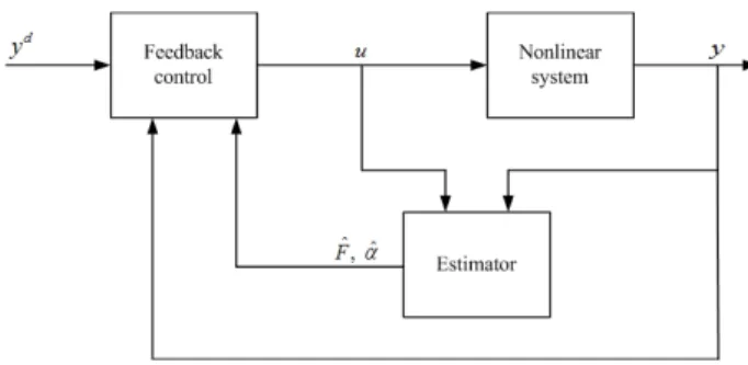
The principle of ultra-local model based control is pre-sented in the Fig. 1. This setting is too general and might not lead to easily implementable tools. This shortcoming is corrected in the following.
2.2. Adaptive PID controllers
Considering the case where ν = 2, equation (2) be-comes as follows:
¨
y (t) = ˆF (t) + ˆα(t) u (t) . (4) Therefore, the loop is closed via an adaptive Proportional-Integral-Derivative controller [20,21], or a-PID, given by
Fig. 1.Ultra-local model control.
the following control law:
u (t) = − ˆF (t) + ¨yd(t) + K pe (t) + KI ∫ e (t) + KDe (t)˙ ˆ α(t) . (5)
Combining (4) and (5) yields to:
¨
e (t) + KDe (t) + K˙ Pe (t) + KI
∫
e (t) = 0. (6) Note that the two functions ˆF (t) and ˆα(t) don’t appear anymore in the equation (6), i.e., the unknown parts and disturbances of the system vanish. We are therefore left with a linear differential equation with constant coeffi-cients of order 3. The tuning of KP, KI and KD
be-comes therefore straightforward to obtain a good tracking of yd(t).
Assume now thatν= 1 in (2): ˙
y (t) = ˆF (t) + ˆα(t) u (t) . (7) The desired behavior is achieved by the adaptive Proportional-Integral controller, or a-PI, defined by:
u (t) = − ˆF (t) + ˙yd(t) + K pe (t) + KI ∫ e (t) ˆ α(t) . (8)
The combination of (7) and (8) gives:
¨
e (t) + KPe (t) + K˙ Ie (t) = 0. (9)
The tracking condition is therefore easily satisfied by an appropriate choice of KPand KI. It boils down to the
sta-bility of a linear differential equation of order 2 with con-stant real coefficients.
3. ONLINE PARAMETER IDENTIFICATION METHODS
3.1. Algebraic derivation method of Fliess-Join
In the first publications on the ultra-local model control [2–4], a recent techniques based on the algebraic deriva-tions of noisy signals [7,8] are applied to estimate the pa-rameter ˆF of the ultra-local model (2). However, the
sec-ond parameterαof the model (2) is considered as constant
;/ Feedback u Non linear y
control system
- i
•
coefficient. Forν= 1, the parameter ˆF (t) is determined
thanks to the knowledge of u (t),αand the estimate of the first order derivative of output signal y which is written as follows: b˙y = −3! T3 ∫ T 0 (T− 2t)y(t)dt, (10) where [0, T ] is quite short time window of estimation which is sliding in order to get the estimate b˙y at each time
instant. At the sampling time kTe(i.e. t = kTe, where Te
denotes the sampling period), the estimate of ˆF is written
as follows:
ˆ
Fk= b˙yk−αuk−1, (11)
where b˙ykis the estimate of the first derivative of the system
output that can be provided at the instant k,αis a constant design parameter, and uk−1 is the control input that has
been applied to the system during the previous sampling time. In practice, the arbitrary choice of the static gain
α present the first point that renders a delicate choice for the adaptive PID control strategy. However, the simulta-neous estimation of the two parameters ˆF and ˆα by other alternative methods can provide a better improvement of results.
3.2. Linear system resolution method
Assuming the numerical control with constant sampling period Tewhich allows to dispose on the system an
avail-able information until the instant kTeand a constant
con-trol uk−1between the two instants (k− 1)Teand kTe. From
the simple model ˙y (t) = ˆF (t) + ˆα(t) u (t), the integration between two sampling instants gives:
yk= yk−1+ ∫ kTe (k−1)Te ˆ F (t) dt + ∫ kTe (k−1)Te ˆ α(t) u (t) dt = yk−1+ ∫ kTe (k−1)Te ˆ F (t) dt + [∫ kTe (k−1)Te ˆ α(t) dt ] uk−1. (12)
Let ˆFk and ˆαk the mean values of ˆF (t) and ˆα(t) in the
interval [(k− 1)Te, kTe]. Finally, we get:
yk= yk−1+ ˆFkTe+ ˆαkTeuk−1. (13)
Considering the following notations:
Yk= yk− yk−1 Te , HkT = [ 1 uk−1 ] , θkT=[ Fˆk αˆk ] , (14)
the previous equation (13) can be written in the following linear system form:
Yk= Hkθk. (15)
Since the regression matrix Hk=
[
1 uk−1
]
has a de-fault rank. Then, this system is always consistent, i.e., rank [Hk] = rank
[
Hk Yk
]
. The aim is to seek at each instant kTethe estimation of the parameter vectorθk.
Ac-cording to the linear system resolution technique detailed in [22], the general expression of estimation is written as follows: θk= Hk{1}Yk+ ( Im+1− Hk{1}Hk ) Λk, (16) where:
• Hk{1}denotes the Moore-Penrose generalized inverse
of Hk, that is mean the matrix X such as HX H = H
[23],
• Λkis an arbitrary matrix of size (m× 1).
The coefficients of matrix Λk appear as degrees of
free-dom that can be used to satisfy other relating constraints to the system control, e.g., optimization constraints. How-ever, these degrees of freedom are equal to the rank of the matrix Im+1− Hk{1}Hk.
Based on the numerical knowledge of ˆF and ˆα, the con-trol input is calculated in (2) as a closed-loop tracking of a reference trajectory t→ yd(t), and a simple cancellation of the nonlinear terms ˆF and ˆα.
3.3. Adaptive observer method
Before formally presenting the adaptive observer algo-rithm, we introduce some transformations on the structure of ultra-local model to properly formulate the problem. In the following, the two cases of ultra-local model, where
ν = 1 andν= 2, are studied. Firstly, consider the case whereν= 1. Then, the ultra-local model (7) can be writ-ten in the following relation:
˙ y (t) = ˆF + ˆαu (t) = u (t) +[ 1 u (t) ][ Fˆ ˆ α− 1 ] . (17)
From the equation (17), the ultra-local model (7) can be represented in the form of a linear time-invariant SISO state-space system as follows (see the work of Q. Zhang [12] for more details about these systems):
˙
x (t) = Bu (t) +Ψ(t)θ,
y (t) = Cx (t) , (18)
where x (t) ∈ R, u(t) ∈ R and y(t) ∈ R are respec-tively the state, input and output of the system, θ = [ ˆ
F αˆ− 1 ]T∈ Rpis a column vector of parameters
as-sumed unknown,Ψ(t) =[ 1 u (t) ]∈ R1×pis a vector of measured signals. In this case, A = 0, B = C = 1 and
Now, consider the case where ν = 2, and assuming the state vector x (t) =[ y (t) y (t)˙ ]T. The ultra-local model (4) is transformed in the following matrix form:
˙ x (t) = [ 0 1 0 0 ] x (t) + [ 0 ˆ F ] + [ 0 ˆ α ] u (t) = [ 0 1 0 0 ] x (t) + [ 0 1 ] u (t) + [ 0 0 1 u (t) ][ ˆ F ˆ α − 1 ] . (19)
From the relation (19), the following linear time-invariant SISO state-space system is obtained. This formalism al-lows us to apply the adaptive observer of Q. Zhang devel-oped in [25]:
˙
x (t) = Ax (t) + Bu (t) +Ψ(t)θ,
y (t) = Cx (t) , (20)
where:
• The matrix A and the vectors B and C are defined by: A = [ 0 1 0 0 ] , B = [ 0 1 ] , C =[ 1 0 ]. • The matrix of measured signals Ψ(t) and the vector
of parameters are given as follows:
Ψ(t) = [ 0 0 1 u (t) ] , θ= [ ˆ F ˆ α− 1 ] .
The design of an adaptive observer is studied in the fol-lowing in order to estimate the state x (t)∈ Rn and the
parametersθ ∈ Rp from the measured signals u (t)∈ R,
y (t)∈ R, Ψ(t) ∈ Rn×p, and the matrices A, B, C. In
prac-tice, it is difficult to check the uniform complete observ-ability [24] of the extended system (20) that should take into account some persistent excitation condition. There-fore, instead of assuming the uniform complete observ-ability of the extended system, the adaptive observer de-veloped in this paper is based on the stabilizability of the matrix pair (A,C) and on some persistent excitation con-ditions, described in the following assumptions Assump-tion 1 and AssumpAssump-tion 2. Noting that the assumpAssump-tions proposed in [25] are designed for MIMO time-varying systems, however, the two following assumptions are re-stricted to SISO systems with constant matrices A, B and
C.
Assumption 1: Assume that the matrix pair (A,C) in system (20) is such that there exists a vector of constant gain K∈ Rnso that the system:
˙
η(t) = [A− KC]η(t) (21)
is globally exponentially stable.
Assumption 2:Letϒ(t) ∈ Rn× Rpbe a matrix of sig-nals generated by a stable filter such as:
˙
ϒ(t) = [A − KC]ϒ(t) + Ψ(t). (22)
Assume thatΨ(t) is persistently exciting so that there ex-ist two positive constantsδ and L such that, for all t, the following inequality is satisfied:
∫ t+L t ϒ
T(τ)CTCϒ(τ) dτ⩾δI (23)
with I∈ Rp× Rpthe identity matrix.
Assumption 1 states that for any given parameterθ, a state observer with exponential convergence can be de-signed for system (20). The gain K sets the estimator dy-namics. Assumption 2 is a persistent excitation condition, typically required for system identification.
Theorem 1: LetΓ ∈ Rp× Rpbe any symmetric
posi-tive definite matrix. Therefore, under Assumptions 1 and 2, the following system of ordinary differential equations:
˙ˆx(t) = A ˆx(t) + Bu(t) +Ψ(t) ˆθ(t)
+[K +ϒ(t)ΓϒT(t)CT][y (t)−C ˆx(t)], (24) ˙ˆ
θ(t) =ΓϒT(t)CT[y (t)−C ˆx(t)] (25) is a global exponential adaptive observer for the system (20).
Remark 1: The matrixϒ(t) is generated by a stable linear filtering of Ψ(t) (for more details, see [12,13]). Typically, the gain vector K is chosen only to ensure the stability of (A− KC), the total gain for the state estima-tion being K +ϒ(t)ΓϒT(t)CT.Γ allows to set the rate of
convergence between the state and the parameters. Remark 2: For any initial conditions x (t0), ˆx (t0), ˆ
θ(t0) and∀θ ∈ Rp, the estimation error ˆx (t)− x(t) tend to zero exponentially fast when t→ ∞.
The proof of theorem 1 requires the following lemma. Lemma 1: Letϕ(t)∈ R×Rpbe a bounded and
piece-wise continuous matrix andΓ ∈ Rp× Rpbe any
symmet-ric positive definite matrix. If there exist positive constants
L,δ such that∀t: ∫ t+L
t ϕ
T(τ)ϕ(τ) dτ⩾δI, (26)
then the system:
˙z(t) =−ΓϕT(t)ϕ(t) z (t) (27)
is exponentially stable.
The lemma of the case with a symmetric positive defi-nite matrixΓ can be proved by simply adapting the proof of [26].
Proof of Theorem 1: For notational convenience, the variables are writing independently of t. The combina-tion of the two adaptive observer equacombina-tions (24) and (25) yields to:
Let ˜x = ˆx− x, ˜θ= ˆθ−θand notice that ˙θ= 0, then: ˙˜x = (A− KC) ˜x+ Ψ ˜θ+ϒ ˜θ. (28) The key step of the proof is to define the following linear combination of ˜x and ˜θ:
η(t) = ˜x (t)− ϒ(t) ˜θ(t) .
After some simple computation, we obtain: ˙
η= (A− KC)η+[(A− KC)ϒ + Ψ − ˙ϒ]θ˜.
Sinceϒ is generated by (22), we simply get: ˙
η= (A− KC)η. (29) By construction (A− KC) is asymptotically stable, so
η → 0 with exponential convergence. Now we should
study the behavior of ˜θ. As ˙θ= 0, we have: ˙˜
θ=ΓϒTCT(y−C ˆx) = −ΓϒTCTC ˜x
=− ΓϒTCTC(η+ϒ ˜θ). (30) Let us first look at the homogeneous part of system (30), that is:
˜
θ=−ΓϒTCTCϒ ˜θ. (31)
SinceΨ is bounded, then ϒ generated from the exponen-tially stable system (22) is also bounded. From the per-sistent excitation condition (23) and by applying Lemma 1 withϕ = Cϒ, (31) is exponentially stable. From the exponential convergences of η and of system (31), we prove that ˜θ → 0 when t → ∞. Finally, from η → 0,
˜
θ→ 0 and the fact that ϒ is bounded, we conclude that
˜
x =η+ϒ ˜θ→ 0 with global exponential convergence. In the following, a practical implementation of the two pro-posed ultra-local model control approaches for a two tank system is given. In the both control techniques, the previ-ous designed adaptive PI controller is considered.
4. TWO-TANK-SYSTEM APPLICATION
4.1. Nonlinear model system
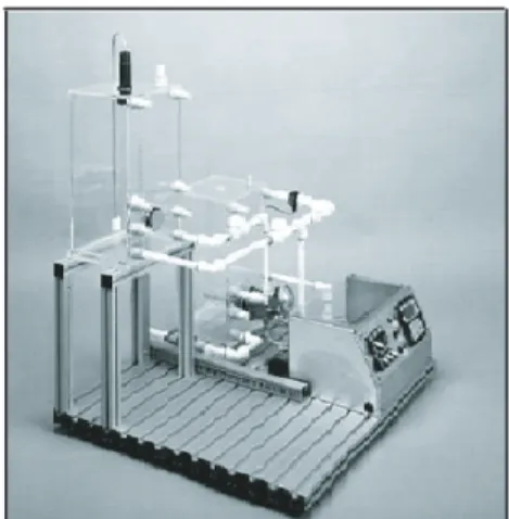
The experimental system used is a two-tank-system de-scribed in Fig. 2. This system consists of a pump and two tanks with orifices and level sensor at the bottom of the upper tank. The pump provides infeed to the upper tank and the outflow of upper tank becomes infeed to the lower tank. In this system, the two identical water tanks have the same section S. Denote by h1(t) the water level in the upper tank, which also represents the system output and h2(t) the water level in the lower tank. The nonlinear model of the considered system is defined by the follow-ing representation: ˙h1(t) =− k1 S √ h1(t) + K SVP(t) , ˙h2(t) = k1 S √ h1(t)− k2 S √ h2(t), (32) Fig. 2.Two-tank-system.
Fig. 3.The experimental setup of acquisition and control system.
where K is the pump constant and VP(t) is the voltage
ap-plied to the pump. The term ki
√
hi(t), i = 1, 2, comes
from the gravity flow. The two parameters k1 and k2 rep-resent the coefficients of the canalization restriction. These two equations are nonlinear due to the presence of the term√h (t), hence the most difficult task in the control
of this considered system will be the control of the water level h1(t) in different operating conditions.
4.2. Control design
For implementing the proposed ultra-local model con-trol, we choose to generate a desired trajectory hd1(t) en-sures a transition from hd1(t0) = 2 V to hd1(tf) = 3 V with
t0= 100 s and tf= 300 s. Fig. 3 displays a full description
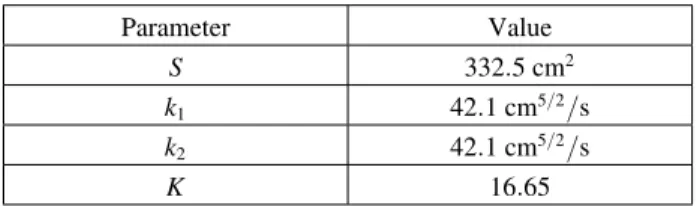
of our acquisition and control system. The pump ensures the filling of the upper tank and it is controlled by a PC which serves as a real-time target to Simulink. The filtered measurements are acquired by the acquisition card PCI-1711. This card provides the communication between the two-tank system and the PC during the running in auto-matic mode. The measurements are filtered by a first order with time constant T . The system parameters are summa-rized in Table 1.
For the experimental applications of control ap-proaches, the same a-PI controllers are implemented
Table 1.Parameter values of the considered system. Parameter Value S 332.5 cm2 k1 42.1 cm5/2/s k2 42.1 cm5/2/s K 16.65
with KP= 20 and KI = 3.5. In the case of linear
sys-tem resolution (LSR) method, we choose Te= 0.1 s and
Λk=
[
−2.5 0.5 ]T
. The parameters of the adaptive observer (AO) based method in the case of ν = 1, are choosen K = 10 andΓ = diag([5,0.05]).
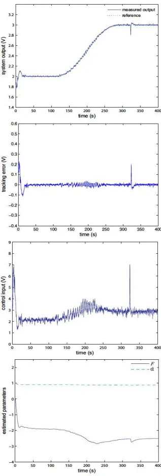
4.3. Experimental results
Figs. 4 and 5 present the experimental results of the pro-posed control approaches. For the experiments, the mea-surements of the level water in the upper tank are filtered by a low pass filter with time constant T = 0.3 s. This filter is added in order to attenuate the influence of the quick fluctuations. At t = 325 s, a level water perturba-tion which simulates a default sensor, is applied directly to the system in order to test the robustness of our pro-posed control approaches. Noting that the same response time is obtained in the different experimental case-studies. This amounts to the choice of the same adaptive controller gains. It is clear that, the water level tracking perfor-mance is provided thanks to the proposed adaptive con-trollers. The ultra-local model control based on adaptive observer, whenν= 1, provides better trajectory tracking performances (see Fig. 5) than the case of linear system resolution (LSR) method. Moreover, the water level per-turbation is quickly and similarly rejected in the different cases of a-PI controllers. In the two figures 4, 5, we can observe the smoothness of the control inputs which have practically the same magnitudes.
Consequently, the good tracking performances and the good robustness towards the level water disturbances are obtained thanks to the proposed adaptive controllers which are based on an online estimation of the two ultra-local model parameters. Noting that the main aim of this paper is not the parameter identification but to obtain in each instant t parameters which satisfies the ultra-local model.
5. CONCLUSIONS
The main contributions of this paper are the design and the application of new ultra-local model control ap-proaches for the water level system. The paper exposes an ultra-local model control with different proposed methods of parameter estimation. The experimental results show that the a-PI controllers approaches are able to ensure good trajectory tracking even in various operating
condi-tions. In addition, the ultra-local model controllers are robust with respect to corrupting noises and external dis-turbances. The most important benefit of this work is the online estimation of the two ultra-local model parameters which provide an improvement in terms of robustness per-formances.
Despite that the proposed control algorithms are in-novative in the field of level water control, good perfor-mances in terms of robustness and tracking are obtained. Due to its robustness and simplicity of implementation, the ultra-local model control appears particularly adapted to industrial environments. Finally, it is straightforward to extend the ultra-local model control approaches to some MIMO systems.
REFERENCES
[1] W. S. Levine, The Control Handbook, Cooperation with IEEE Press, New York, 1996.
[2] M. Fliess and C. Join, “Commande sans modèle et com-mande Ã˘a modèle restreint,” e-STA, vol. 4, no. 5, pp. 1-23, 2008.
[3] M. Fliess and C. Join, “Model-free control and intelligent PID controllers: towards a possible trivialization of non-linear control?,” Proc. of 15th IFAC Symposium on System
Identification, SYSID’2009, Saint-Malo, vol. 15, pp.
1531-1550, 2009.
[4] M. Fliess and C. Join, “Model-free control,” International
Journal of Control, IJF’2013, vol. 86, no. 12, pp.
2228-2252, 2013.
[5] M. Fliess, C. Join, and S. Riachy, “Revisiting some prac-tical issues in the implementation of model-free control,”
Proc. of 18th IFAC World Congress, Milan, pp. 8589-8594,
2011.
[6] F. Lafont, J.F. Balmat, N. Pessel, and M. Fliess, “Model-free control and fault accomodation for an experimen-tal greenhouse,” Proc. of International Conference on
Green Energy and Environmental Engineering (GEEE-2014), Tunisia, 2014.
[7] M. Fliess and H. Sira-Ramírez. “An algebraic framework for linear identification,” ESAIM Control Optimization and
Calculus of Variations, vol. 9, pp. 151-168, 2003. [click]
[8] M. Fliess and H. Sira-Ramírez, “Closed-loop parametric identification for continuous-time linear systems via new algebraic techniques,” In H. Garnier & L. Wang (Eds):
Identification of Continuous-time Models from Sampled Data, pp. 363-391, 2008.
[9] H. Sira-Ramírez, C. G. Rodríguez, J. C. Romero, and A. L. Juárez, Algebraic Identification and Estimation Methods in
Feedback Control Systems, Wiley Series in Dynamics and
Control of Electromechanical Systems, 2014.
[10] H. Thabet, M. Ayadi, and F. Rotella, “Towards an ultra-local model control of two-tank-system,” International
Journal of Dynamics and Control, vol. 4, no. 1, pp. 59-66,
· · · ···· reference 3.2 - -measured output ~ 2.8 ~ 2.6 £l-6 2.4 E S! 2.2 ~ 2 1.8 1.6 1.4 0 so 100 150 200 250 300 350 400 tlme(s) 0.6 0.5 0.4 0.3 ~
g
0.2 Q) 0.1 C) _i;; -"'~
0 -0.1 -0.2 -0.3 -0.4 0 50 100 150 200 250 300 350 400 time(s) g 8 7 ~ 6g_
5 .!: 2 4 c 0 0 3 2 50 100 150 200 250 300 350 400 time (s) s~ - ~ - - ~ - - ~ - - ~ - ~ - - ~ - - ~ - ~ - - -ft 4 - - - -d -4 -5 . _ _ __. _ _ _,_ _ _ _,_ _ _ .._ _ __. _ _ _,_ _ _ ... _ __, 0 so 100 150 200 250 300 350 400 tlme(s)Fig. 4. Experimental results in the case of linear system
resolution method. - -measured output 3.2 ··· mference ~ 2.8 ~ 2.6 £l-6 2.4 E
*
2.2 i;';' 1.8 1.6 1.4 0 so 100 150 200 250 300 350 400 time (s) 0.6 0.5 0.4 0.3 ~g
0.2•:
.
~
Q) 0.1 C) _i;; -"' 0j
V''
.
-0.1 -0.2 -0.3 -0.4 0 50 100 150 200 250 300 350 400 time(s) 9 8 7 - 6 ~1
s .!:e
4 c 0 0 3 2 so 100 150 200 250 300 350 400 time (s) - - -F - - - -d -3 -4' - - - ' - - - ' - - - - ' - - - . . _ _ __. _ _ _,_ _ _ ... _ __, 0 so 100 150 200 250 300 350 400 tlme(s)Fig. 5. Experimental results in the case of adaptive
[11] H. Thabet, M. Ayadi, and F. Rotella, “Ultra-local model control based on an adaptive observer,” Proc. of IEEE
Con-ference on Control Applications (CCA), Antibes, 2014.
[12] Q. Zhang, “Adaptive observer for multiple-input-multiple-output (MIMO) linear time-varying systems,” IEEE
Trans-actions on Automatic Control, vol. 47, pp. 525-529, 2002.
[click]
[13] Q. Zhang and A. Clavel, “Adaptive observer with expo-nential forgetting factor for linear time varying systems,”
Proc. of 40th IEEE Conference on Decision and Control (CDC), IEEE Control Systems Society, vol. 4, pp.
3886-3891, 2001.
[14] A. M. Ali and Q. Zhang. “Adaptive observer based fault diagnosis applied to differential-algebraic systems,” In 5th
IFAC Symposium on System Structure and Control,
Greno-ble, 2013.
[15] I. D. Landau, Adaptive Control: The Model Reference
Ap-proach, Marcel Dekker, New York, 1979.
[16] M. Fliess, J. Lévine, P. Martin, and P. Rouchon, “Flatness and defect of non-linear systems: introductory theory and examples,” International Journal of Control, vol. 61, no. 6, pp. 1327-1361, 1995. [click]
[17] J. Haggège, M. Ayadi, S. Bouallègue, and M. Benre-jeb, “Design of fuzzy flatness-based controller for a DC drive,” Control and Intelligent Systems, vol. 38, pp. 164-172, 2010.
[18] F. Rotella, F. J. Carrilo, and M. Ayadi, “Digital flatness-based robust controller applied to a thermal process,” Proc.
of IEEE International Conference on Control Application,
Mexico, pp. 936-941, 2001.
[19] V. Volterra and J. Pérès, Théorie générale des
fonction-nelles, Gauthier-Villars, 1936.
[20] K. J. Aström and T. Hägglund, Advanced PID Controllers,
Instrument Society of America, Research Triangle Park,
North Carolina, 2nd edition, 2006.
[21] A. O’Dwyer, Handbook of PI and PID Controller Tuning
Rules, 3rd edition, Imperial College Press, London, 2009.
[22] F. Rotella and P. Borne, Théorie et pratique du calcul
ma-triciel, Éditions Technip, Paris, 1995.
[23] A. Ben-Israel and T. N .E. Greville, Generalized Inverses:
Theory and Applications, John Wiley and Sons, 1974.
[24] A.H. Jazwinski, “Stochastic Processes and Filtering The-ory,” in Mathematics in Science and Engineering, Aca-demic, New York, vol. 64, 1970.
[25] Q. Zhang, Adaptive observer for MIMO linear time
varying systems, Technical Report 1379, IRISA, ftp://ftp.irisa.fr/techreports/2001/PI-1379.ps.gz, 2001. [26] B. D. Anderson, R. R. Bitmead, C. R. J. Johnson, P. V.
Kokotovic, R. L. Kosut, I. M. Mareels, L. Praly, and B. D. Riedle, Stability of Adaptive Systems: Passivity and
Aver-aging Analysis, series in Signal Processing, Optimization,
and Control, Cambridge, MIT Press, MA, 1986.
Hajer Thabet received her Master diploma in Automatic and Signal Pro-cessing in 2011 from Ecole Nationale d’Ingénieurs de Tunis (ENIT), Tunisia. From 2011 to 2015, she joined the Lab-oratoire de Recherche en Automatique LA.R.A. (ENIT) and the Laboratoire Génie de Production LGP (ENIT, France) where her research interests are focused on identification methods of ultra-local models for dynamic systems control. She received her Ph.D. degree in Electrical Engineering from ENIT in 2015.
Mounir Ayadigraduated from Ecole Na-tionale d’Ingénieurs de Tunis in 1998 and received his PhD degree in Auto-matic Control from the Institut National Polytechnique de Toulouse in 2002. He was a post-doctoral fellow at the Ecole Supérieure d’Ingénieurs en Génie Elec-trique de Rouen in 2003. He is currently Maître de Conférences at the Ecole Na-tionale d’Ingénieurs de Tunis and the head of Electrical Engi-neering Department in ENIT. His research interests are in the area of control system theory, predictive and adaptive control, and at systems.
Frédéric Rotella was born in 1957. In 1981, he received the diploma in Engineer-ing from the Institut Industriel du Nord (Lille, France). From 1981 to 1994, he joined the Laboratoire d’Automatique et d’Informatique Industrielle de Lille where his research interests are focused on mod-elization and control of non linear systems. He received the Ph.D. degree (in 1983) and the Doctorat d’Etat degree (in 1987) from the University of Sci-ence and Technology of Lille-Flandres-Artois. During this pe-riod, he served at the Ecole Centrale de Lille (ex. Institut In-dustriel du Nord) as Assistant Professor in Automatic Control. In 1994, he joined the Ecole Nationale d’Ingénieurs de Tarbes (France) as Professor of Automatic Control. From this date he is in charge of the Department of Electrical Engineering of this engineering school. His personnal fields of interest are about control of non linear systems and time-varying linear systems. Professor Rotella is member of the Club EEA. Professor Rotella is coauthor of Théorie et pratique du calcul matriciel (1995, ed. Technip, Paris, France).