Dense gas-particle suspension upward flow used as heat transfer fluid in solar receiver: PEPT experiments and 3D numerical simulations

(1)

Open Archive TOULOUSE Archive Ouverte (OATAO)

OATAO is an open access repository that collects the work of Toulouse researchers and

makes it freely available over the web where possible.

This is an author-deposited version published in :

http://oatao.univ-toulouse.fr/

Eprints ID : 17294

To link to this article : DOI : 10.1016/j.powtec.2016.11.006

URL :

http://dx.doi.org/10.1016/j.powtec.2016.11.006

To cite this version :

Ansart, Renaud and García-Triñanes, Pablo

and Boissière, Benjamin and Benoit, Hadrien and Seville, Jonathan

and Simonin, Olivier Dense gas-particle suspension upward flow

used as heat transfer fluid in solar receiver: PEPT experiments and

3D numerical simulations. (2017) Powder Technology, vol. 307. pp.

25-36. ISSN 0032-5910

Any correspondence concerning this service should be sent to the repository

administrator:

staff-oatao@listes-diff.inp-toulouse.fr

(2)

Dense gas-particle suspension upward flow used as heat transfer fluid in

solar receiver: PEPT experiments and 3D numerical simulations

Renaud Ansart

a,

_*

_{, Pablo García-Triñanes}

b

_{, Benjamin Boissière}

a

_{, Hadrien Benoit}

a

_,

Jonathan P.K. Seville

b

_{, Olivier Simonin}

c

a_{Laboratoire de Génie Chimique, Université de Toulouse, CNRS, INPT, UPS, Toulouse, France}

b_{Department of Chemical and Process Engineering [J2], University of Surrey, GuildfordGU2 7XH, United Kingdom} c_{Institut de Mécanique des Fluides de Toulouse (IMFT), Université de Toulouse, CNRS, INPT, UPS, Toulouse, France}

Keywords: Fluidization PEPT CFD simulation Euler-Euler

Dense particle suspension Solar receiver

Heat transfer fluid

A B S T R A C T

A dense particle suspension, also called an upflow bubbling fluidized bed, is an innovative alternative to the heat transfer fluids commonly used in concentrated solar power plants. An additional advantage of this technology is that it allows for direct thermal storage due to the large heat capacity and maximum temper-ature of the particle suspension. The key to the proposed process is the effective heat transfer from the solar heated surfaces to the heat transfer fluid, i.e. the circulating solid suspension. In order to better understand the process and to optimise the design of the solar receiver, it is of paramount importance to know how particles behave inside the bundle of small tubes. To access to the particle motion in the solar receiver, two different techniques are carried out: experimental using positron emission particle tracking (PEPT) and 3D numerical simulation via an Eulerian n-fluid approach with NEPTUNE_CFD code. Both numerical predictions and PEPT measurements describe an upward flow at the centre of the transport tube with a back-mixing flow near the wall which influences the heat transfer mechanism. Comparisons between experiment and computation were carried out for the radial profiles of the solid volume fraction, and vertical and radial time-averaged and variance velocities of solid, and demonstrating the capability of NEPTUNE_CFD code to simulate this peculiar upflow bubbling fluidized bed.

1. Introduction

Conventional Heat Transfer Fluids (HTF) used in solar power plants have many drawbacks, in particular a limited working temperature domain. A solution to overcome these drawbacks uses solid particles as the HTF. In a new patented concept [11], it is proposed to use a dense particle suspension, also called an upflow bubbling fluidized bed, as the HTF, flowing upwards in an array of tubes at the focus of the solar receiver. The solids can also be used as an energy storage medium. The present study reports work car-ried out within a FP7 EC project CSP2, http://www.csp2-project.eu, aimed at developing this alternative HTF in order to extend the work-ing temperature. The use of high temperature heat transfer fluids allows operating at high temperature thermodynamic cycles such as super critical and combined cycles in associated steam turbines. Dense particle suspensions will enable operating temperatures over

*Corresponding author.

E-mail address:renaud.ansart@ensiacet.fr(R. Ansart).

1000◦_{C limited only by the construction materials of the receivers,}

compared with 560◦_{C for the most efficient molten salts currently}

used, thus increasing the plant efficiency and decreasing the cost per produced kWh. In addition, this new HTF has no lower tempera-ture limitation. Flamant et al.[10]have demonstrated the capacity of dense gas-particle suspensions to transfer concentrated solar power from a tubular receiver to an energy conversion process by acting as a HTF. A mean value of heat transfer coefficient corresponding to 400 W/m2K has been measured for standard operating conditions at low temperature and much higher values, up to 1100 W/m2_{K, were}

measured at temperatures up to 750◦_C_[1]_.

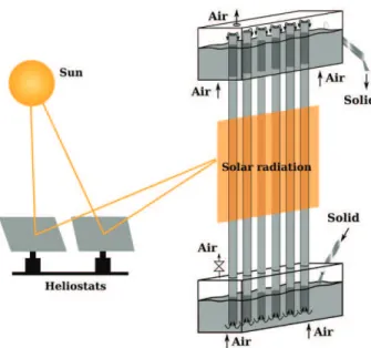
The solar receiver consists of one or more multi-tube exchangers, which are the absorbing modules for the solar radiation. The number of exchangers depends on the power of the receiver, and also on the heliostat field configuration. The walls of the tubes are heated by the concentrated solar radiation, and solid particles in dense suspension circulate inside them (Fig. A.1). Boissière et al.[3]have studied the hydrodynamics of upward flow of a gas-solid dense suspension at ambient temperature, in a vertical two tube bundle of small diameter tubes (diameter 34 mm), which have their bases immersed in a

(3)

Fig. A.1. Schematic view of a module of the solar receiver with dense upward solid flow.

slightly pressurized fluidized bed. The results obtained confirmed that it is possible to ensure stable upward flow of dense gas-solid suspensions in a bundle of tubes in parallel. Operating conditions for stable upward flows of the suspension and an equal repartition of the total solid flow rate between the tubes were determined experi-mentally. Boissière et al.[3]demonstrated that the suspension at the inlet is under minimum fluidizing conditions at any solid flow rate. Hence, the gas velocity in the tube is the sum of the aeration velocity and the minimum fluidization velocity.

The key to the proposed process is effective heat transfer from the solar heated surfaces to the heat transfer fluid, i.e. the cir-culating solid suspension. In order to understand this fully and so optimise the design of the solar receiver, it is of paramount importance to know how particles behave inside the bundle of small tubes within it. Indeed, the radial movement induces par-ticle renewal at the wall, and determines the amount of heat removed from the wall to the bulk of the bed. To access to the particle motion in the solar receiver, two different tech-niques (experimental and numerical) are employed in this study. Measurement of particle motion in opaque suspensions such as this is difficult since conventional optical methods cannot be applied. Positron emission particle tracking (PEPT) is used here since it is the only non-intrusive method that is capable of giv-ing detailed information on the particle circulation within the tubes.

The two CFD approaches commonly used for exploring flu-idized bed systems are Eulerian-Lagrangian and Eulerian-Eulerian models. In the Eulerian-Lagrangian approach, particles are mod-elled as discrete elements and the Newtonian equations of motion for each individual particle are solved, with inclusion of the effects of particle collisions and forces acting on the particles due to the gas [32]. The particle-particle and particle-wall interactions may be accounted for in a deterministic manner rather than stochastic. This method is computationally expensive when the number of real particles to be tracked is high (more than 1010 _{particles in}

our geometry). The silicon carbide particles used are less than 100lm in diameter, so considering the solar receiver dimensions

more than several billion of particles have to be considered. As the computation demands are considerable and limiting, the Eulerian-Lagrangian approach is limited to simulation of lab-scale fluidized beds with large particles. In the Eulerian-Eulerian model, the two

phases are treated as interpenetrating continua and separated but coupled mass, momentum and energy Eulerian transport equations are written for the fluid and particle phases. The kinetic theory of granular flow and frictional theory are used to describe the rheol-ogy of the particle phase. This model is the most frequently used approach for predicting the dynamic behavior of fluid particle sys-tems on a large scale up to and even including commercial-scale reactors[8].

The aim of this study is to examine the capability of the math-ematical models implemented in NEPTUNE_CFD code to predict the behavior of an upflow bubbling fluidized bed by comparison with very accurate experimental measurements and to enhance the understanding of the physical mechanisms involved. The goal is to achieve the couple the hydrodynamics and the heat transfer in order to optimise the design of the solar receiver.

2. Experimental description: PEPT technique

Positron emission particle tracking (PEPT) is a technique for tracking a single radioactive tracer particle. It allows non-invasive observation of the motion of a single particle within a dense bed of similar particles. PEPT uses positron emitting radioisotopes which have the unique attribute that their decay leads to simultaneous emission of a pair of back-to-backc-rays. From the detection of a

small number of such pairs the tracer position can be determined by triangulation. As a result accurate tracking is possible even in very dense systems involving significantc-ray attenuation and scattering.

Using the positron camera at the Positron Imaging Centre (University of Birmingham) a SiC tracer particle moving in the upflow bubbling fluidized bed can be located by PEPT to within 0.5 mm (in 3 dimensions). The PEPT technique employs an itera-tive algorithm[22]to discard outlying data arising from scattered radiation. Once the parameters of the algorithm are selected, the tracking of a tracer particle for an extended period of time in a closed, circulating system builds up an integrated picture of particle behavior at each point in space and this allows the visualisation of the particle behavior and reconstruction of maps of axial and radial movement, circulation times and pseudo-density (using the PEPT “occupancy” function). The resulting locations are of the form (tk, xk,

yk, zk).

The tracers can be produced either by direct irradiation of the sample in a cyclotron, converting oxygen in the sample directly to

18_{F, or by irradiation of water, which is then exchanged with, or}

attached to, molecules on the surface of the tracer. SiC hardly adsorbs

18_{F; therefore in a separate project a technique was developed}

for depositing a very thin layer of Al2O3 on SiC tracer particles

under ambient conditions using gas-phase deposition in a fluidized bed[30]. The core-shell particles produced were identical in proper-ties that affect the hydrodynamic behavior in the bed (density, shape and size). The density comparison between uncoated SiC and the sample coated with 40 cycles is detailed in[30]. A density differ-ence of 0

.

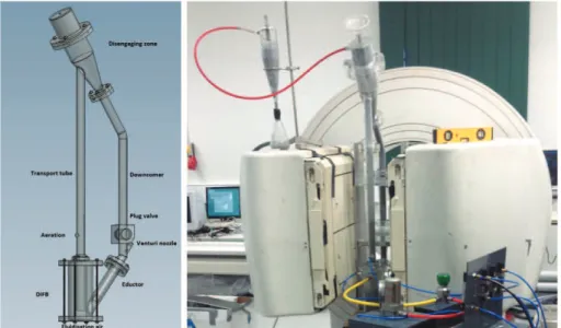
8% is measured, which is a negligible difference. A single tracer particle was then mixed with other SiC particles and added to the Dispenser Fluidized Bed (DiFB). The tracer is supposed to be representative of all the particles of the bed, these are treated as statistically indistinguishable and therefore the trajectories are considered equivalent. In order to obtain sufficient experimental data it was necessary to operate this rig in a continuous circula-tion mode so that sufficient passes of the radioactive tracer could be observed. A Geiger counter was used to detect the particle as it entered the uplift transport (length 1.1 m) to check that the tracer particle was circulating in the experimental loop. A sketch of the single 30 mm ID tube in the circulating experimental rig is shown inFig. A.2(left). On the right a photo depicts the disposition

(4)

Fig. A.2. Schematic drawing of the experimental rig (left) and location of the single tube circulating apparatus positioned relative to the detectors (right).

Table A.1

Experimental conditions. *Between y=150 mm and 250 mm above the aeration, where y is the vertical coordinate with respect to the bottom of the PEPT camera.

Umf Umb Fluidization velocity Aeration velocity Fluidization flowrate Aeration flowrate Venturi nozzle flowrate Net solids mass flux*

(mm/s) (mm/s) (m/s) (m/s) (Nm3_/h) _(NL/h) _(NL/h) _(kg/s/m2₎

5 8 0.096 0.04 4.0 190 48 27.2

of the set-up during the PEPT experiments, with the two positron “cameras” on each side.

The dense upward-flowing suspension rises up the transport tube, which has additional aeration, and terminates in a cyclone-like disengaging zone. From here the disengaged solids fall under gravity into a downcomer. It is necessary to feed particles from the downcomer into the pressurized DiFB in a controlled way using a purpose-designed venturi nozzle [13]. In the experiments, the PEPT camera was able to locate and track particles over a height of 500 mm, from the top of the DiFB, including the region situated just before the aeration port. In this way it was possible to obtain a distribution of all locations in the transport tube over a typical 2-h experimental run (half life of18_{F = 110min).}

For purposes of comparison with the simulation results a region situated 10 cm above the aeration port will be considered here. The operating parameters including aeration flow rate of the uplift trans-port tube, air flow in the venturi and fluidisation flow rate were selected to ensure steady flow of solid in the tubes, so that the results have high statistical significance, as reported in previous experi-ments[13]. The flow in the vertical tubes is greatly influenced by the fluidisation flow rate of the DiFB and the amount of aeration introduced directly to the tube.Table A.1summarizes the operating conditions for the experiments carried out in this study, which were kept constant.

The position data were generated in a Cartesian coordinate system, which is convenient for viewing projections on the coordi-nate planes.Fig. A.3shows an example of a tracer particle moving upwards with time, where y is the vertical coordinate. As in related work on bubbling beds by Stein et al.[27], vertical motion consists of a series of vertical “jumps” which are associated with bubble motion, interspersed with quiescent periods in which the particle may descend in the downward-flowing dense phase between bubbles. The information obtained from PEPT yields a continuous trajectory of a single labelled particle while present in the field of view.

During this PEPT experiment, the tracking precision of a 68lm

tracer reaches 0.85 mm in 3D with a location frequency of 10 Hz for a tracer moving at 0.2 m/s. Acrylic perspex was chosen specifically for the construction of the apparatus for this experiment because of its low gamma ray attenuation. The length of the tube is 500 mm and the precision was found to be at least 0.6 mm[13]. (Tracking can still be performed in apparatus of higher attenuation, but precision is then reduced.). 0 1000 2000 3000 4000 5000 6000 7000 8000 −100 0 100 200 300 400 500 Time, ms Vertical coordinate, mm

X, Y, Z locations over time

X Y Z

Fig. A.3. Example of individual trajectory against time (Fluidization velocity= 0.096m/s, Aeration velocity=0.04m/s).

(5)

2.1. Determination of solid volume fraction

Let us define a cylindrical grid of annular cells, the occupancy of each cell ‘ Oc′_{being defined as the fraction of the overall}

experimen-tal duration tTwhich the tracer spends in each cell and is given by:

Oc =

Pnpass

n=1tcell,n

tT

(1) wheretcell,nis the single-pass residence time of the particle for pass

n in a given cell. npass is the total number of passes through the

cell during the experiment. If we assume that all the particles are statistically indistinguishable (ergodicity) then Oc can be written as the ratio of Ncellthe mean number of particles in the cell to NTthe

total number of particle in the tube:

Oc =Ncell NT

(2) The time outside the field of view is also tracked and it represents on average between 3 and 4.5 times the time spent inside the transport tube depending on the experimental conditions.

The mean solid volume fraction of particle is calculated as fol-lows: ap= Ncell•m_p qp•v_cell = NT•Oc•m_p qp•v_cell = Oc•M_T qp•v_cell (3)

where mpis the mass of one particle, MTis the overall mass of the

powder contained in the system and vcellrepresents the volume of

the cell considered.

The calculation of the time-average value for each corresponding element in the circumference gives the plot presented inFig. A.8.

2.2. Determination of time-averaged Eulerian solid velocity

To diminish the effect of the individual location error on the velocity determination, the local instantaneous particle velocities are calculated using an interpolation from six subsequent particle locations. The particle velocity in direction i at the kth particle track location, up,i(tk), is calculated from successive values of location, Pk,i

the ith component of the point in space at time tk:

1 µ_P k,i− Pk−5,i tk− tk−5 ¶ (4) The 6-point method used for PEPT introduces some smoothing (particularly in chaotic/turbulent systems) but reduces the overall error in velocity calculations. The instantaneous tracer particle velocity can be calculated according to Eq. (4). For overlapping sets, the tracer particle velocity is obtained by comparing 11 consecu-tive locations[28] and performing a weighted rolling average by replacing each data point with the average of the neighbouring six estimates of the resulting velocities.

During each loop, the tracer particle left the detectable range, because the PEPT detectors only covered approximately 500 mm of the transport tube. Therefore, the readings immediately before exit and after return of the particle were discarded for the purposes of velocity determination. The velocity is subsequently assigned to the cell considering the interpolation over 11 consecutive locations of the tracer particle which reduces the effect of PEPT measurement error on the results.

Finally, the time-averaged particle velocity is given by:

Up,i= 1 nmeas nmeas X i=1 up,i(tk) (5)

where nmeasis the number of measurements in the cell.

The time-variance of solid phase velocity is defined as follows:

s2 p,i= 1 nmeas nmeas X n=1 (u′ p,i)2 (6)

where up,i′= up,i(tk) − Up,iis the solid fluctuating velocity.

The locations in PEPT occur at random time intervals due to the random nature of radioactive decay, and due to the inefficiencies in detection. The average value of velocity error for PEPT is reasonable due to the six-point-averaging method, however the standard devia-tion of the error for this particular set of data is 0.2 m/s. The locadevia-tion precision has been dominated by errors in the z direction (0.6 mm) because of the low number of detection elements along the axis[13]. This filter will smooth the data by removing high-frequency events however it may be too restrictive in the case of the radial component. 3. Numerical simulation description: Euler n-fluid approach

Three-dimensional numerical simulations are carried out using the code NEPTUNE_CFD. This Eulerian n-fluid unstructured par-allelized multiphase flow software has been developed in the framework of the NEPTUNE project financially supported by CEA (Commissariat à l’Energie Atomique), EDF (Electricite de France), IRSN (Institut de Radioprotection et de Sureté Nucléaire), and AREVA-NP[18]. The modelling approach for poly-dispersed fluid-particle flows is implemented by the Institut de Mécanique des Fluides de Toulouse (IMFT) in the NEPTUNE_CFD V1.08 version. The numerical solver has been developed for High Performance Computing[20,21].

3.1. Mathematical models

The Eulerian n-fluid approach used is a hybrid method [19]in which the transport equations are derived by phase ensemble aver-aging for the continuous phase and by use of the kinetic theory of granular flows supplemented by fluid effects for the dispersed phase. The momentum transfer between gas and particle phases is mod-elled using the drag law of Wen and Yu[31], limited by the Ergun[6] equation for dense flows[9,14]. The collisional particle stress tensor is derived in the frame of the kinetic theory of granular media[2]. In the present study the gas flow equations are treated as laminar because the gas Reynolds stress tensor in the momentum equation is neglected compared to the drag term. For the solid phase, a trans-port equation for the particle random kinetic energy, q2

p, is solved.

The gas-particle turbulent correlation is negligible. The effects of the particle-particle contact force in the very dense zone of the flow are taken into account in the particle stress tensor by the additional frictional stress tensor[26].

3.2. Numerical parameters 3.2.1. Geometry

The geometry is that used by Boissière et al. [3]simplified to access to the gas pressure drop in a longer tube. Only one tube of the solar receiver was simulated and the volume of the pressurized flu-idized bed was divided by two. The tube diameter for the simulation is 34 mm instead of 30 mm for the PEPT experiments. As the two tube diameters are very close, the authors believe that this difference does not have a significant effect on the hydrodynamics.

(6)

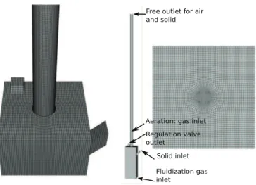
Fig. A.4. 3D mesh for the numerical simulation 1,650,000 cells.

3.2.2. Mesh

The mesh (Fig. A.4) is composed of 1,650,000 hexahedra, based on the O-grid technique with approximatelyDr = 1

.

2 mm and

Dz = 1

.

5 mm. The DiFB has a horizontal sectional area of 0.04 m2

(20 cm X 20 cm), a height of 40 cm and is equipped with a lateral solid entrance. A tube of 2.05 m height and 34 mm in internal diam-eter has its lower end submerged in the DiFB to a distance of 10 cm from the gas distributor. Secondary air injection, hereafter termed “aeration”, is set at 57 cm from the bottom of the tube.

3.2.3. Phase properties

The properties of the SiC particles used for the experimental mea-surements are presented inTable A.2. The experiments were carried out at ambient temperature and the fluidization gas was air.

Fig. A.5shows the silicon carbide particles. It can be observed that the particle are strongly non-spherical and polydispersed. The first simulations carried out using the Sauter diameter of the particle size distribution (PSD) showed that the numerical results strongly underestimated the bed suspension void fraction. This result could be explained by reference toFig. A.6which shows predictions for the bed void fraction at a given multiple of the minimum fluidiza-tion velocity as a funcfluidiza-tion of particle diameter; “classical” drag law predictions due to Wen and Yu, and Ergun are shown and assume homogeneous expansion. The point shown is for the experimental value of the void fraction under these conditions. Clearly this is not consistent with the predictions, possibly because of the combina-tion of shape factor and size distribucombina-tion effects. To take into account

Fig. A.5. SEM photograph of silicon carbide particles.

dp (µm)

30 40 50 60 70 80 g 0.4 0.45 0.5 0.55 0.6 0.65 0.7

Wen and Yu for spherical particle Ergun

Wen and Yu for C_shape= 1, f_shape=3.2

g exp=0.59

Fig. A.6. Evolution of the void fraction of a dense fluidized bed of silicon carbide parti-cles by assuming an homogeneous expansion for a fluidization velocity Vf= 2×Umf=

10mm/s.

the non-sphericity of particles in the drag term Loth[17]proposed a correction to the Wen and Yu drag law using the coefficients (Cshapeand fshape):

Re∗_p=CshapeRep fshape , (7) C∗ d= Cd Cshape

.

(8)

where Rep = agqg|Ev_lgr|pdp is the particle Reynolds number. The

spheroidal shape factor f_shapeis inversely proportional to the change in terminal velocity since the drag dependence is linear in creeping flow (Rep). It ranges from 1 for a sphere to 1.19 for a tetrahedron.

Cshapecan be thought of as a Newton-drag correction. It ranges from

1 for a sphere to 4.5 for a tetrahedron.

Fig. A.7. Instantaneous field of solid volume fraction. On the left: an overall view of the geometry, at the center: a cross section view at the center of the column and on the right: enlargement of the cross sectional view of the bottom part.

(7)

r/R

0

0.2

0.4

0.6

0.8

1

p

0.32

0.34

0.36

0.38

0.4

0.42

0.44

0.46

0.48

0.5 Simulations 10 cm above aeration

Simulations 50 cm above aeration

Experiments 10 cm above aeration

Fig. A.8. Radial profile of time-averaged solid volume fraction at 10 cm above the aeration level.

In the creeping flow regime Rep≪ 1, as encountered in this study,

the parameter to take into account is fshape. According to the Wen and

Yu drag law,Fig. A.6shows that a value of f_shapeof 3.2 over range of Loth value recommended.

Hence for the numerical simulations, the classical drag laws with-out shape correction have been retained by assuming a monodis-persed mean diameter of 40lm for the silicon carbide particles.

This mean diameter predicts a void fraction for homogeneous bed expansion in good agreement with the experimental measurement.

The gas density is a function of gas pressure and obtained by following the ideal gas law with a constant temperature of 293K.

The phase properties used for the simulation are summarized in Table A.3.

3.2.4. Boundary conditions

The geometry is composed of three inlets:

• The fluidization gas distributor, which is a wall for the par-ticles and where an air flow rate of 2.268 kg/h is imposed. This air flow rate corresponds to a superficial gas velocity of 1

.

66cm/s ≈ 3 × Umf, where Umf is the minimum fluidization

velocity.

• The lateral injection of solid in the DiFB with a solid flow rate imposed of 25

.

5kg/s/m2(relative to the tube surface) with a

Table A.2

Properties of SiC used in the experiments. The PSD is determined by the Malvern Mastersizer2000 using a laser diffraction method. The minimum fluidization velocity Umf, the minimum bubbling

velocity Umband their associated void fractions

agmfandambwere experimentally determined by

the Davidson and Harrison [5] method.

Parameter Value d10 44lm d50 79lm d90 130lm d32 64lm Particle density 3210kg/m3 Umf 5 mm/s ag,mf 0.57 Umb 8 mm/s ag,mb 0.59 Table A.3

Phases properties used for the numerical simulation.

Parameter Value

Gas density P = 101325Pa 1.204kg/m3

Gas viscosity 1.85.10−5_Pa•s

Particle diameter 40lm

Particle density 3210kg/m3

solid volume fraction of 0.5. The gas mass flow rate imposed by this injection is extremely low relative to the other gas flows at 5

.

209•10−9kg/s which corresponds to a gas velocity of 4 cm/s

in the tube as for the experimental rig.

• The aeration is a gas inlet set at 56.4 cm from the lower end of the tube where a gas mass flow rate of 5

.

3875•10−5kg/s is

imposed.

The superficial gas velocity in the tube is equal to 4.5 cm/s= 9Umf

(sum of both aeration and gas coming from DiFB as discussed above). The geometry is also composed of two outlets with an imposed pressure equal to atmospheric pressure: the top of the tube is a free outlet for air and particles, and an outlet placed at the top of the DiFB imitates the regulation valve. The pressure regulation valve is mod-eled as a pressure loss implemented on the cells of the valve conduit introduced so as to keep a constant pressure inside the DiFB equal to the atmospheric pressure plus 240 mbar.

The wall-type boundary condition is no-slip for the two phases.

3.3. Simulation progress

The numerical simulations have been performed on parallel com-puters with 140 cores. A numerical simulation is divided into two steps: a transitory step to reach a predicted constant total mass of particles in the column (solid mass flow rate injected equal to solid mass flow rate leaving the geometry) and an established regime during which the statistics are computed for 400 s. The time-average of the solid flow variablewpis defined by:

wp(X) = P n wp (X, tn)ap(X, tn)Dtn P n ap (X, tn)Dtn (9)

and the time-variance by:

w′ p(X)2= h wp(X, tn) − wp(X) i2 (10) whereapandqpare respectively the volume fraction and the density

of the particle, andDt the time step.

4. Results and discussion

The numerical results for gas pressure drop along the tube are in very good agreement with the experimental measurements obtained by Boissière et al.[3](Table A.4). As can be noticed, the numerical simulations predict perfectly the decrease of the gas pressure due to the aeration. Below the aeration, the mean solids volume fraction is equal to 43% and this decreases to 36% above the aeration. This decrease of the solids volume fraction can be observed inFig. A.7. The

Table A.4

Time-averaged gas pressure drop at the wall on 50 cm height.

Exp. data[3] Numerical results

Below the aeration 136 mbar/m 135 mbar/m

(8)

r/R

0 0.2 0.4 0.6 0.8 1 U p,y (m/s) -0.2 -0.15 -0.1 -0.05 0 0.05 0.1 0.15 0.2 0.25

Simulations 10 cm above aeration Simulations 50 cm above aeration Experiments 10 cm above aeration

(a) Vertical component of solid velocity.

r/R

0 0.2 0.4 0.6 0.8 1 p p U p,y (kg/s/m 2) -300 -200 -100 0 100 200

(b) Vertical solids mass flux.

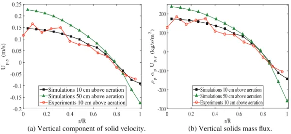
Fig. A.9. Radial profiles of time-averaged vertical velocity and mass flux of solid phase at 10 cm above the aeration point.

solid is injected into the DiFB from the right side of the geometry. The height of solid in the DiFB is controlled by the pressure imposed at the surface of the bed.

4.1. Experimental vs. simulation results

The PEPT measurements and the numerical predictions are com-pared as radial profiles of flow variables extracted at 10 cm above the aeration level. This position, imposed by the experimental mock-up, is close to the aeration and we can presume that the flow is not fully stabilized. As the simulated tube is about two meters in height, the influence of the distance from the aeration is also dis-cussed. The numerical predictions are plotted at 10 cm and 50 cm above the aeration. As the diameters of tubes used in the exper-iment and in the simulation are not exactly the same (30 mm for the experiment and 34 mm for the numerical simulation) the radial position is normalized by the tube radius. Moreover, owing to the axisymmetry of the tube receiver, the time-averaged flow may be assumed to obey cylindrical symmetry. So, spatial averag-ing of the time-averaged variables was performed in the azimuthal direction.

Fig. A.8shows the radial profile of the solids volume fraction. PEPT measurements and numerical predictions both present a mini-mum at the center of the tube and a maximini-mum near the wall. These results are in relatively good agreement with a slight over-prediction from the model. When the distance from the aeration increases, the solid volume fraction decreases. Indeed, the size and velocity of the bubbles increase as a function of the height in the tube which increases the bed expansion.

Fig. A.9shows the vertical component of the solids phase velocity and the associated solids mass flux defined as the product of this ver-tical velocity, the solids volume fraction and the solids density. The numerical results and the experimental data for the vertical compo-nent of solid flux are similar, with a maximum value at the center and a negative minimum close to the wall; this is due to bubble rise in the center of the tube.

Fig. A.10shows the solids velocity vectors with the field of solid volume fraction in background. An upward flow in the center of the tube and a downward more concentrated solid flow near the wall are clearly observed. A rotating vortex can be observed near the wall. This trend is the same as that normally observed in dense bubbling fluidized beds[12]. In the present study, the time-averaged solids flow direction reverses at approximatively 78% of the tube radius. This downward flow has a strong influence on the behavior

of the heated dense particle suspension inside the solar receiver. Indeed, the particle suspension will be heated prior to reaching the irradiated area by the hot flow coming from the upper zone. This is confirmed by the temperature measurements conducted by the authors’ partners in an experimental solar receiver[1]. It can be noticed, that the downward solid mass flux is slightly overestimated by the numerical simulations. The extrema of the solid mass flux, as does the velocity, increase as a function of the height in the tube due to the increase of the bubbles velocity.

Fig. A.11presents the upward and absolute values of downward mean vertical solids mass flux. At 10 cm above the aeration, the downward solids mass flux is very low but not zero at the center of tube, at about 25 kg/s/m2, and very high at the wall, at about 180 kg/s/m2. This trend of downward vertical solids mass flux is the reverse of the upward solids mass flux with a maximum at the center of the tube and minimum near the wall. With the increase of the height in the tube, the downward solid mass flux decreases at the center of the tube while the upward solid mass flow increases. At the wall, the reverse phenomenon is observed. The ratio between the upward and the downward solid mass flux does not change with the increase of the distance from the aeration.

Fig. A.10. Time-averaged solid vector velocity with selected pathline of particle, and solid volume fraction for a section of the riser tube between 45 cm and 50 cm above the aeration point predicted by numerical simulations.

(9)

r/R

0

0.1

0.2

0.3

0.4

0.5

0.6

0.7

0.8

0.9

1 Vertical solid mass flux (kg/s/m

2

)

0

50

100

150

200

250

300

350 Upward solid mass flux 10 cm above aeration

_{Downward solid mass flux 10 cm above aeration}

Upward solid mass flux 50 cm above aeration

Downward solid mass flux 50 cm above aeration

Fig. A.11. Radial profile of time-averaged upward and absolute value of downward solids mass flux at 10 cm above the aeration level.

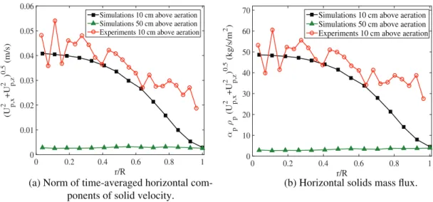
Fig. A.12shows the norm of the time-averaged horizontal com-ponents of solids velocity (qU2

p,x+ U2p,z, x and z are the

direc-tions perpendicular to the gravity direction), which corresponds to the time-averaged radial velocity by assuming that the azimuthal component of solids velocity is equal to zero by axisymmetry of the geometry, and the associated solids mass flux. The numerical predictions and experimental results are in good agreement in the central part of the tube. However, a discrepancy can be observed near the wall. Indeed, the experimental measurements do not tend to zero at the wall probably due to the error location reported in the horizontal z direction as mentioned before. The simulations seem more realistic as far as the horizontal radial velocity is concerned. It should also be noted that the comparison is made very close to the aeration point, where the flow is not fully established. Thus, the norm of horizontal solids velocity is not equal to zero. It is also noteworthy that the numerical value of this velocity decreases very fast a few tens of centimeters above the aeration point and tends to zero. The horizontal velocity is three times lower than the ver-tical one in the center of the tube; the flow is not isotropic and predominantly vertical. The horizontal solids mass flux decreases,

as does the velocity, from the center to equal zero at the wall. However, the simulation results seem to decrease faster than the experimental data near the wall. This radial movement of the par-ticle is very important for heat exchange between the wall and the particle suspension, in order to avoid “hot spot” developing at the wall.

Fig. A.13presents radial profiles of vertical and horizontal com-ponents of time variance of solids phase velocity. In the numerical approach the solids velocity time variance is the sum of a predicted part (

<

up,x′up,x′

>

,

<

up,y′up,y′

>

,

<

up,z′up,z′

>

) which corresponds

to the collective motion of particles and a modelled uncorrelated part (q2

p). This last part is less than 10−5m2

/

s2and could be negligible

compared to the fluctuations of the predicted solid velocity. The PEPT data and numerical simulations are in good agreement for the vertical variance. Thus, the numerical simulations are able to predict the vertical mixing of the particles well. At the center of the tube the standard deviation of the vertical component of solids veloc-ity is of the same order (≈ 0

.

2 m/s) as the time-averaged vertical solids velocity. This means that the instantaneous particle veloc-ity can be negative at the center leading to non-zero downward

r/R 0 0.2 0.4 0.6 0.8 1 (U p,x 2 +U p,z 2 ) 0.5 (m/s) 0 0.01 0.02 0.03 0.04 0.05 0.06

(a) Norm of time-averaged horizontal

com-ponents of solid velocity.

r/R 0 0.2 0.4 0.6 0.8 1 p p (U p,x 2 +U p,z 2 ) 0.5 (kg/s/m 2 ) 0 10 20 30 40 50 60 70

(b) Horizontal solids mass flux.

(10)

r/R

0 0.2 0.4 0.6 0.8 1

Variance of solid velocity (m

2 /s 2 ) 0 0.01 0.02 0.03 0.04 0.05 0.06

(a) Vertical component.

r/R

0 0.2 0.4 0.6 0.8 1

Variance of solid velocity (m

2 /s 2 ) 0 0.005 0.01 0.015 0.02 0.025 0.03 0.035 0.04

(b) Horizontal component.

Fig. A.13. Radial profiles of time variance of solids phase velocity at 10 cm above the aeration point.

solids mass flux as shown in Fig. A.11. However, the variance in the horizontal velocity is largely overestimated by the simulation. PEPT measurements show a variance of the horizontal velocity much lower than in the vertical direction. This anisotropy of the parti-cle velocity fluctuations is not represented by the numerical results which overestimate the radial mixing. In contrast, the numerical simulations show that the particle velocity fluctuations are almost isotropic at the center of the tube and tend to be anisotropic near the wall.

4.2. Discussing the plausible reasons of discrepancy

As discussed above, the mathematical models that underpin the numerical simulation approach of this study are able to predict the behavior of an upflow bubbling fluidized bed in the solar receiver. Nonetheless, some discrepancies have been observed such as an overestimation of the downward solids mass flux by the numerical simulation.

To improve the simulation approach several tracks can be followed. First of all, it is important to consider the differences between the experimental and numerical geometries. The tube diameter for the numerical simulations was 34 mm in the simulation instead of 30 mm for the experimental solar receiver and its length was 2.06 m instead of 1.1 m. A mesh refinement was tested on a sim-plified fluidization column with the same diameter, the same particle properties and showed no effect on the bed expansion. However, a refinement of the mesh, especially in the radial direction, could improve the prediction of the downward flow near the wall.

Clearly, the treatment of the particles in the simulation is grossly simplified, making use of a single diameter of an (effectively) spherical particle to describe a size distribution of extremely non-spherical particles. As discussed above, the particle diameter was arbitrarily decreased in order to match the bed expansion measured by experiments but this method can be only a stopgap. One draw-back of this diameter reduction is that the particle-particle collisions are not well described. Many studies were recently carried out in the literature[4,15,17,29]to take into account the non-sphericity of particles in the formulation of drag coefficients. A 3D characteriza-tion by experimental measurement of irregularly shaped particles used in the study (Fig. A.5) is tricky but the way to model it still remains a challenge.

To reduce the over-prediction of downward solids mass flux near the wall, one possibility would be to increase the friction of the particles at the wall through adjustment of the wall-particle

boundary condition, but the wall-particle boundary condition fric-tion is already at the maximum through the no-slip condifric-tion used. Another possibility would be to increase the particle-particle friction. The model used in this study[26]contains several param-eters but the authors have retained the use of recommended value. Nonetheless, other models to describe frictional stress could be used. For example, Farzaneh et al.[7]have recently shown that the results of a visco-plastic model proposed by Jop et al.[16]are in better agreement with the experiments for prediction of the bed hydrodynamics and the movement of the fuel particles than the models of Sundaresan[26]and Schaeffer[24]conventionally used for CFD simulation.

5. Conclusions

The positron emission particle tracking technique and an Eulerian n-fluid approach were used in this work to shed light on dense par-ticle suspension motion in an upflow bubbling fluidized bed applied as a heat transfer fluid in solar receiver. The objectives were not only to measure the properties of the system but also the test the util-ity of the computational model, which might then be used in future design work for this technology. Comparisons of the time averaged radial profiles of solid volume fraction, vertical and radial velocity and velocity variance of particles present satisfactory agreement and demonstrate the capability of NEPTUNE_CFD software to predict this peculiar upflow bubbling fluidized bed.

Although a strong assumption was made on drag term, the simulation was successful in predicting the axial gas pressure drop and the effect of a secondary air injection on this profile. Simulation also succeeded in reproducing the radial evolution of the vertical and horizontal solid velocity and the time variance of the solids vertical velocity which controls the axial mixing. Both numerical predictions and PEPT measurements describe an upward flow at the centre of the transport tube due to rising bubbles with a back-mixing flow near the wall which will strongly influence the solar to particles heat transfer mechanism. When compared to the experimental data, simulation predicts a slightly higher solid downward flow near the wall. The observed discrepancies between the experimental and sim-ulation results were mainly attributed to the simplified treatment in the model of the nature of the particles.

Future numerical simulations will investigate the coupling between the hydrodynamics of the dense particle suspension and the heat transfer to reproduce the experiments conducted in the solar furnace.

(11)

Nomenclature

Roman symbols

Cd drag coefficient (−)

dp particle diameter (m)

ec particle-particle normal restitution coefficient (−)

g gravitational constant (m•s−2)

g₀ _{radial distribution function (−)}

I_g→p,i Interphase momentum transfer (kg•m−2•s−2)

Kp granular diffusivity (m2•s−1)

Kcol

p collisional granular diffusivity (m2•s−1)

Kkin

p kinetic granular diffusivity (m2•s−1)

mp particle mass (kg•_m−3₎

np particle number density(m−3)

Pg mean gas pressure (N•m−2)

q2

p mean particle random kinetic energy (m2· · ·−2)

Rep particle Reynolds number (−)

Uk,i mean velocity of phase k (m•s−1)

Umf minimum fluidization velocity (m•s−1)

uk,i′ fluctuating velocity of phase k (m•s−1)

Vd drift velocity (m•s−1)

Vf superficial gas velocity (m•s−1)

Vr relative gas-particle velocity (m•s−1)

Vt terminal settling velocity (m•s−1)

Greek symbols

ak volume fraction of phase k (−)

amax

p maximum solid packing k (−)

lg gas viscosity (kg.m−1

.

s−1)

lp particle viscosity (kg.m−1

s)

qk density of phase k (kg.m−3)

Sk,ij effective stress tensor of the phase k (kg•m−1•s−2)

Scol

k,ij collisional stress tensor of the phase k (kg•m−1•s−2)

Sfric

k,ij frictional stress tensor of the phase k (kg•m−1•s−2)

Skin

k,ij kinetic stress tensor of the phase k (kg•m−1•s−2)

tc collisional timescale (s)

tF

gp mean gas-particle relaxation timescale (s)

Subscripts

g gas

p particle

Acknowledgements

This work was developed in the frame of the CSP2 European project. The authors acknowledge the European Commission for cofunding the “CSP2” Project Concentrated Solar Power in Particles -(FP7, project N 282 932). This work was granted access to the HPC resources of CALMIP under the allocation P1132 and CINES under the allocation gct6938 made by GENCI.

Appendix A. NEPTUNE_CFD mathematical equations

The Eulerian n-fluid approach used is a hybrid method, in which the transport equations are derived by phase ensemble averaging for the continuous phase and by using kinetic theory of granular flows supplemented by fluid and turbulent effects for the dispersed phase, thanks to a joint fluid-particle probability density function (PDF) approach.

In the following equations, subscript k = g refers to the gas phase and k = p or q to the particle phase.apqpin the particle transport

equation represent npmpwhere npis the number density of particle

centers and mpis the mass of a single particle: ap = npmpqp is an

approximation of the local volume fraction of particle p. Hence, gas and particle volume fractions,agandaphave to satisfy:

ag+ap= 1 (A.1)

Mass transport equation:

∂

takqk+

∂

xj

akqkUk,j= 0 (A.2)

whereqkis the density of k-phase and Uk,iis the i−component of its

velocity.

Momentum transport equation

xj (A.3) where Pg is the mean gas pressure, gi is the gravity i−component.

I_g→pare the interphase momentum transfer between particle and gas without the mean gas pressure contribution andSk,ijis the effective

stress tensor of phase k.

Interphase transfer modelling:

According to the particle to gas density ratio, the dominant forces between the gas phase and particles are the drag and Archimedes’ force, so the mean momentum gas-particle transfer term may be written:

I_g→p,i_{= −I}_p→g,i_{= −}apqp tF gp Vrp,i (A.4) 1 tF gp =3 4 qg qp |Evr|p dp Cd(Rep) (A.5) Cd(Rep) = (Cd,WY if ag≥ 0

.

7

min£Cd,WY, Cd,Erg¤else ag

<

0

.

7

(A.6) Cd,WY=    24 Rep ³ 1 + 0

.

15Re0.687 p ´ a−1.7 g Rep

<

1000 0

.

44a−1.7 g Rep≥ 1000 (A.7) Cd,Erg= 200(1 − ag ) Rep +7 3, Rep=ag qg|Evr|pdp lg (A.8)

Vrp,i=

<

vr,i

>

p= Up,i− Ug,i− Vdp,i (A.9)

Vdp,iis the drift velocity which can appear due to turbulence[25]or

sub grid effect[23]which is assumed to be negligible (due to the inertia of the particles).

(12)

Particle stress modelling: S_p,ij= Skin

p,ij+ Scolp,ij+ S frict

p,ij (A.10)

Skin

p,ij+ Scolp,ij=

_U p,i

∂

xi ¸2 (A.24) Particle random kinetic energy transport equation:

suspension in tube, Sol. Energy 118 (2015) 622–633.

[2] A. Boëlle, G. Balzer, O. Simonin, Second-order prediction of the prediction of the particle-phase stress tensor of inelastic spheres in simple shear dense suspensions, In Gas-Particle flows, ASME FED 28 (1995) 9–18.

[3] B. Boissière, R. Ansart, D. Gauthier, G. Flamant, M. Hemati, Experimental hydro-dynamic study of gas-particle dense suspension upward flow for application as new heat transfer and storage fluid, Can. J. Chem. Eng. 93 (2) (2015) 317–330.

[4] R. Clift, J.R. Grace, M.E. Weber, Bubbles, Drops, and Particles, Courier Corpora-tion. 2005.

[5] J. Davidson, D. Harrison, R. Jackson, Fluidized Particles: Cambridge University Press, 1963. 155 pp. 35s, 1964.

[6] S. Ergun, Fluid flow through packed columns, Chem. Eng. Prog. 48 (1952) 89–94.

[7] M. Farzaneh, A.-E. Almstedt, F. Johnsson, D. Pallarès, S. Sasic, The crucial role of frictional stress models for simulation of bubbling fluidized beds, Powder Technol. 270 (2015) 68–82.

[8] P. Fede, H. Neau, O. Simonin, I. Ghouila, 3D unsteady numerical simulation of the hydrodynamic of gas phase polymerization pilot reactor, 7th International Conference on Multiphase Flows., 2010,

[9] P. Fede, O. Simonin, A. Ingram, 3D numerical simulation of a lab-scale pres-surized dense fluidized bed focussing on the effect of the particle-particle restitution coefficient and particle-wall boundary conditions, Chem. Eng. Sci. 142 (2016) 215–235.

[10] G. Flamant, D. Gauthier, H. Benoit, J.-L. Sans, R. Garcia, B. Boissiere, R. Ansart, M. Hemati, Dense suspension of solid particles as a new heat transfer fluid for concentrated solar thermal plants: On-sun proof of concept, Chem. Eng. Sci. 102 (2013)

[11] G. Flamant, M. Hemati, FrenchPatent No.1058565, 20 October 2010. PCT Exten-sion, 26 April 2012, No. WO2012/052661 A2, 2016, 2015.

[12] F. Fotovat, R. Ansart, M. Hemati, O. Simonin, J. Chaouki, Sand-assited flu-idization of large cylindrical and spherical biomass particles: experiments and simulation, Chem. Eng. Sci. 126 (2015) 543–559.

[13] P. García-Triñanes, J. Seville, B. Boissière, R. Ansart, T. Leadbeater, D. Parker, Hydrodynamics and particle motion in upward flowing dense particle suspensions: application in solar receivers, Chem. Eng. Sci. 146 (2016) 346–356.

[14] A. Gobin, H. Neau, O. Simonin, J. Llinas, V. Reiling, J. Sélo, Fluid dynamic numer-ical simulation of a gas phase polymerization reactor., Int. J. Numer. Methods Fluids 43 (2003) 1199–1220.

[15] A. Hölzer, M. Sommerfeld, New simple correlation formula for the drag coefficient of non-spherical particles, Powder Technol. 184 (3) (2008) 361–365.

[16] P. Jop, Y. Forterre, O. Pouliquen, A constitutive law for dense granular flows, Nature 441 (2006) 727–730.

[17] E. Loth, Drag of non-spherical solid particles of regular and non regular shape, Powder Technol. 182 (2008) 342–353.

[18] N. Méchitoua, M. Boucker, J. Laviéville, J. Hérard, S. Pigny, G. Serre, An unstruc-tured finite volume solver for two-phase water/vapour flows modelling based on elliptic oriented fractional step method, NURETH 10, Seoul South Korea, 2003,

[19] S. Morioka, T. Nakajima, Modeling of gas and solid particles two-phase flow and application to fluidized bed, J. Theor. Appl. Mech. 6 (1) (1987) 77–88.

[20] H. Neau, P. Fede, J. Laviéville, O. Simonin, High Performance Computing (HPC) for the Fluidization of Particle-Laden Reactive Flows, The 14th International Conference on Fluidization, From Fundamentals to Products, Noordwijkerhout, Netherlands, 2013,

[21] H. Neau, J. Laviéville, O. Simonin, Neptune_CFD High Parallel Computing Per-formances for Particle-Laden Reactive Flows, 7th International Conference on Multiphase Flow, ICMF 2010, Tampa, FL, May 30 - June 4, 2010,

[22] D. Parker, C. Broadbent, P. Fowles, M. Hawkesworth, P. McNeil, Positron emission particle tracking-a technique for studying flow within engineering equipment, Nucl. Instrum. Methods Phys. Res., Sect. A 326 (3) (1993) 592–607.

[23] J. Parmentier, O. Simonin, O. Delsart, A functional subgrid drift velocity model for filtered drag prediction in dense fluidized bed, AIChE 58 (4) (2011) 1084–1098.

[24] D.G. Schaeffer, Instability in the evolution equations describing incompressible granular flow, J. Differ. Equ. 66 (1) (1987) 19–50.

(13)

[25] O. Simonin, E. Deutsch, J. Minier, Eulerian prediction of the fluid/particle correlated motion in turbulent two-phase flows, Appl. Sci. Res. 51 (1993)

[26] A. Srivastava, S. Sundaresan, Analysis of a frictional kinetic model for gas/particle flows, Powder Technol. 129 (2003) 72–85.

[27] M. Stein, Y. Ding, J. Seville, D. Parker, Solids motion in bubbling gas fluidised beds, Chem. Eng. Sci. Vol. 55 (22) (2000) 5291–5300.

[28] R. Stewart, J. Bridgwater, Y. Zhou, A. Yu, Simulated and measured flow of gran-ules in a bladed mixer-a detailed comparison, Chem. Eng. Sci. 56 (19) (2001) 5457–5471.

[29] S. Tran-Cong, M. Gay, E.E. Michaelides, Drag coefficients of irregularly shaped particles, Powder Technol. 139 (1) (2004) 21–32.

[30] D. Valdesueiro, P. Garcia-Triñanes, G. Meesters, M. Kreutzer, J. Gargiuli, T. Leadbeater, D. Parker, J. Seville, J. van Ommen, Enhancing the activation of silicon carbide tracer particles for PEPT applications using gas-phase deposi-tion of alumina at room temperature and atmospheric pressure, Nucl. Instrum. Methods Phys. Res., Sect. A 807 (2016) 108–113.

[31] C. Wen, Y. Yu, Mechanics of fluidization, Chem. Eng. Symp. Ser. 62 (1965) 100–111.

[32] J. Xie, W. Zhong, B. Jin, Y. Shao, Y. Huang, Eulerian-Lagrangian method for three-dimensional simulation of fluidized bed coal gasification, Adv. Powder Technol. 24 (1) (2013) 382–392.