Measurement of magnetic hysteresis swelling-up with frequency: impact on iron losses in electric machine sheets

O

pen

A

rchive

T

OULOUSE

A

rchive

O

uverte (

OATAO

)

OATAO is an open access repository that collects the work of Toulouse researchers and

makes it freely available over the web where possible.

This is an author-deposited version published in :

http://oatao.univ-toulouse.fr/

Eprints ID : 18285

To link to this article :

DOI: 10.1109/ECMSM.2017.7945864

URL :

http://dx.doi.org/10.1109/ECMSM.2017.7945864

To cite this version :

Giraud, Alexandre and Bernot, Alix and Lefevre, Yvan

and Llibre, Jean-François Measurement of magnetic hysteresis swelling-up

with frequency: impact on iron losses in electric machine sheets. (2017) In:

ECMSM 2017 (International Workshop of Electronics, Control,

Measurement, Signals and their application to Mechatronics), 24 May 2017

- 26 May 2017 (Donostia, Spain).

Any correspondence concerning this service should be sent to the repository

administrator:

staff-oatao@listes-diff.inp-toulouse.fr

Measurement of magnetic hysteresis swelling-up with

frequency: impact on iron losses in electric machine

sheets

A. Giraud, A. Bernot

Y. Lefevre and J.F. Llibre

Toulouse, France

yvan.lefevre@laplace.univ-tlse.fr, jean-francois.llibre@laplace.univ-tlse.fr

Abstract—This paper relates to the measurement and the modeling of iron losses in electric machines by studying the influence of frequency on magnetic hysteresis. Indeed, increasing frequency involves a swelling-up of the hysteresis loop, influencing several magnetic properties and so iron losses. The proposed study is to characterize a FeSi NO20 steel sheet under sinusoidal waveform at different level of magnetic flux density by varying the frequency. The measurements provide information about the magnetic behavior under frequency variation. Then, iron losses are decomposed to highlight their different components, as hysteretic or eddy current losses. The perspective of the study is to improve a quasi-static model of hysteresis based on the play model by turning it into a dynamic one. Finally, taking into account dynamic effect involves a far better accuracy of iron losses modeling.

Keywords—Electric machine, Iron losses, Magnetic hysteresis measurements, high speed actuators, frequency dependency.

I. INTRODUCTION

The iron losses have been studied for decades, especially in electric machines [1]. Following the development of power electronics and new controlling systems such as Pulse Width Modulation (PWM), the use of electrical machines evolved. Higher speed and so higher frequencies can be reached, leading to a large type of applications and reducing the size of actuators for the same power. The increase of frequencies induces a high iron losses growth [2]. Therefore, concerning electrical actuator design, the prediction of iron losses is essential, especially at high frequency levels.

In order to improve the existing models, measurements of the variation of the magnetic hysteresis with the frequency have to be done. Indeed, an increase of the frequency involves a swelling-up of the hysteresis loop at constant magnetic flux density and so an increase of iron losses. The more accurate that swelling-up is measured, the more precise the dependency between frequency and iron losses is quantifiable. Thus, for several levels of magnetic flux density, iron losses in electrical steel sheets are measured by varying the frequency. Moreover, frequency has a huge impact on several magnetic quantities [3], such as coercivity or maximum magnetic applied field [4].

These quantities are directly related to the swelling-up of the hysteresis with frequency.

A standard hysteresis-graph (MPG-200) is used as magnetic field source and regulation system. A sinusoidal waveform of magnetic flux density is obtained by regulating the corresponding applied magnetic field. The measurements are made on NO20 electrical steel sheets which are commonly used in electric machines. In this way, the dynamic effects of the magnetic hysteresis are analyzed in order to determine their influence on both magnetic flux density and magnetic field intensity. Combining dynamic and DC measurements, the static hysteresis is isolated. Adding a simple eddy current losses modeling based on uniform field in the sheet, it is possible to characterize the general magnetic behavior of the sheet under sinusoidal excitation.

II. EXPERIMENT DETAILS

A. Set-up and material used

The measurements are made on a single electrical steel sheet of NO20 (60x60mm) composed of a ferromagnetic alloy (FeSi – 4%Si). Its Physical properties are given in Table 1. The sample is magnetized by a single sheet tester (SST) supplied by a regulation system. The total system is called a hysteresis-graph. The regulation system imposes the supply current of the primary winding of the SST and so the magnetic field H inside the sample is determined by a current measurement. The current needed is regulated through a voltage regulation, so a magnetic flux density B regulation. More precisely, the waveform of B (frequency, magnitude, shape) is specified and the voltage in the secondary winding of the SST is regulated to reach this point by supplying the corresponding current in the primary winding. The generated magnetic flux circulates in an oversized back-iron. Therefore, the SST provides the magnetization in the sheet and serves as sensor for regulation system. Sheet and SST are presented on Fig. 1.

TABLE I: Properties of NO20 sheet used for the study

Size Thickness Density Resistivity 60x60mm 0.2mm 7650 kg.m3 _6x10-8_Ω.m

Fig. 1: Single sheet tester and NO20 steel sheet

B. Measurement process

First, to characterize the frequency influence, sinusoidal waveforms of B are preferable to determine the general behavior easily. Thus, we measure different magnetic quantities by varying the frequency from 0 to 5000Hz at several level of magnetic flux density B. These levels (0.5T, 0.9T, 1T, 1.1T and 1.4T) are chosen in order to reproduce material magnetization under different conditions. The real saturation level of NO20 is around 1.7T. However we have decided to limit the B magnitude at 1.4T to ensure all the measurements for each frequency. Indeed, reaching the saturation at frequencies above 1kHz requires higher current supply; that is not possible in our set-up due to the current limit of our power supply.

Then, DC hysteresis loops are measured for every B level. They allow the identification of the NO20 static behavior. Indeed, these measurements are independent of the frequency and correspond to the hysteretic behavior of losses in magnetic materials.

III. ANALYSIS OF THE FREQUENCY INFLUENCE

A. General results of the measurements

First, magnetic quantities such as maximum magnetic field and coercive magnetic field are measured by the MPG-200. Those quantities are good indicators of the swelling-up of the hysteresis loop with frequency, observable on Fig. 2. They directly traduce the shape of the loop.

Fig. 3 shows the variation with the frequency of the maximum field reached at each level of B. Except for 0.5T, a gap is observed at a specific frequency for each level. The higher is the magnitude of B, the lower is the frequency of the

gap. It is far more visible for 1.4T, which can be explained by the proximity of the saturation level. For 0.5T, the magnitude seems too low to observe the gap. Moreover, the variation of maximum H is chaotic before the gap for 1T, 1.1T and 1.4T, but linear after the gap for each level of B. For lower B, the variation of maximum H is also linear before the gap.

Fig. 4 presents the variation of coercive field with frequency. This variation appears as a polynomial one for each level of B. However, as for maximum field, a gap is observed at the same frequencies for 0.9T, 1T, 1.1T and 1.4T. Therefore, reaching the maximum value of H and withstanding the demagnetization (coercivity) seems harder just before that gap frequency. Just after the gap, maximum H and coercive H suddenly drop.

Fig. 2: Swelling-up of hysteresis with frequency

Fig. 3: Variation with frequency of maximum value reached by H field (A/m) at each B level

Fig. 4: Variation with frequency of coercive H field (A/m) at each B level

Fig. 5: Variation with frequency of iron losses at each B level

This phenomenon is also highlighted on Fig. 5 which displays the variation of iron losses in the sheet with frequency, for the same levels of B. The same observations are possible with the iron losses as with the coercive field. The variation seems to be polynomial, and the gap is not visible at 0.5T. Obviously, coercive field and iron losses are linked to the maximum value of magnetic field, explaining why the gap is also observed on Fig. 4 and Fig. 5. The gap frequencies are gathered in Table II.

The frequency changes with the magnitude of B but the behavior around the gap is the same: additional investigation is needed.

TABLE II: Measured gap frequencies

B magnitude (T) 0.9 1 1.1 1.4 Frequency (Hz) ~ 2850 ~ 2650 ~ 2450 ~ 1850

B. Investigations on magnetic “gap”

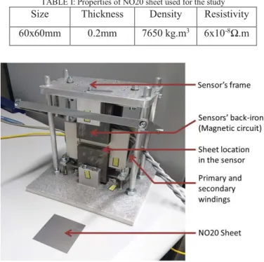
In order to ensure that the device is giving the same level of

B around the gap, the hysteresis loops at 1.4T for 1800Hz and

1900Hz are presented in Fig.6. This gap (Fig. 3, 4 and 5) could be some sort of magnetic resonance, but such a phenomenon has only been observed at several GHz in thin film (0.5µm) of materials [5]. Here, we study electrical steel sheet with a 0.2mm thickness. As far as we know, it is the first time such an observation is made on frequency measurements in ferromagnetic steel sheet. However, it is possible to dismiss the resonance of the frame because we should have the same resonance frequency for each level of B in this case (especially for 0.9T, 1T and 1.1T). Indeed, the variation of B is not important enough to impact such a variation of resonance frequency in the SST frame. Nevertheless, to ensure the validity of this assumption, measurements with conditions have to be done.

Fig. 6: Hysteresis loops around the gap (1800Hz before – 1900Hz after) at 1.4T

C. Investigations based on electrical measurements

First, electrical measurements (Peak to peak secondary voltage Vpp and peak to peak primary current Ipp) were processed to ensure the values given by the regulation system. From voltage and current measurements, B and H are easily obtained in the sheet. The flux in the air is also calculated and subtracted to B. In this way, we can compare data from regulation system and extern electrical measurements. The set-up is presented in Fig.7 and the values are given in Table III and Table IV at 1.4T B magnitude.

TABLE III: Electrical measurements at 1.4T B from MPG200 (T) Hmax from MPG200 (A/m) Frequency (Hz) Peak to peak secondary voltage (V) Peak to peak primary current (A) 1,396 816,2 500 4,27 1,72 1,406 827,72 1000 8,53 1,81 1,395 789,92 1800 15,63 1,72 1,410 219,28 1900 11,29 0,48 1,397 223,72 2000 11,77 0,497 1,398 235,481 2200 12,93 0,525 1,399 253,12 2500 14,67 0,565 1,405 283,14 3000 17,83 0,631 1,407 307,45 3499 20,66 0,693 1,399 337,13 4000 23,94 0,767 1,406 361,13 4500 26,65 0,820

TABLE IV: Calculated magnetic values from electrical measurements at 1.4T

Frequency (Hz) Magnetic air flux density (T) Calculated B in the sheet (T) Calculated Hmax in the sheet (A/m) 500 0,014097 1,403 782,63 1000 0,01480 1,399 822,18 1800 0,014059 1,426 780,54 1900 0,003945 0,982 219,04 2000 0,004070 0,972 226 2200 0,004304 0,969 239 2500 0,004629 0,968 257 3000 0,005165 0,979 286,7 3499 0,005674 0,974 315,04 4000 0,006243 0,986 346,63 4500 0,006717 0,975 372,91

According to the measurements, the B never reached its set point after the gap. That is why the maximum magnetic field is so low: the regulation of the MPG200 failed.

To avoid a power supply default, the H corresponding to

B = 1.4T before the gap (1800Hz) and after the gap (1900Hz)

can be imposed. Actually, B sinus is regulated with a maximum

H criterion. The B will be then measured and compared to the

value of Table III. The proposed measurements are gathered in Table V.

TABLE V: Magnetic measurements for imposed H

Imposed Hmax (A/m) Frequency (Hz) B measured (T) Hmax for B = 1,4T@1800Hz 789,92 1800 2,099 1900 2,089 Hmax for B = 1,4T@1900Hz 219,28 1800 1,45 1900 1,4

The B measured in the sheet is not realistic, proving that the hysteresis-graph regulation and measurement loop are not working properly. Besides, electrical measurements allow verifying the values for B and H in Table VI.

TABLE VI: Calculation of magnetic values from electrical measurements

Measured B (T) Vpp (V) Calculated B (T) Ipp (A) Calcultated Hmax (A/m) 2,099 18,74 1,71 1,73 788,90 2,089 19,56 1,69 1,71 779,09 1,45 10,80 0,99 0,48 218,18 1,4 11,09 0,96 0,48 219,54 Here, the value of calculated B is possible in a NO20 steel sheet. Therefore, the device can provide enough power supply but failed regulating it. The question is now why it failed. Due to the dependency of the gap frequency with B, we cannot assess that the regulation issue is only a software issue.

D. Mechanical set-up investigations

To determine whether the gap is influenced by sample’s geometry, we decided to test not only one sheet, but also a stack of sheets (loose lamination, not assembled). The magnetic behavior of several sheets, providing a larger volume of sample, is different that for a single sheet. If the gap is changing with such parameters, it could be an argument for a mechanical vibration influence. Moreover, adding a non-magnetic adhesive tape in the center of the sheet could also provide information. The different tests are displayed in Table VII at 1.4T B magnitude.

TABLE VII: Mechanical set-up tests at 1.4T

Mechanical conditions Frequency (Hz) Hmax (A/m) Fall of Hmax (%) 1 sheet 1800 815,24 72,2 1900 219,28 2 sheets 1800 216,89 25,6 1900 161,32 3 sheets 1800 193,05 25,3 1900 144,2 4 sheets 1800 177,22 22,4 1900 137,57 5 sheets 1800 153,12 23,1 1900 117,68 8 sheets 1800 142,48 20,9 1900 112,73 1 sheet with adhesive tape 1800 1340,2 80,9 1900 255,97

To complete the investigations, measurements are made at 1.4T on a M250-35A steel sheet, which has a thickness of 0.35mm but barely the same resistivity and density than NO20. The results presented in Table VIII confirm a gap but around 1050 Hz. Electrical measurements were also made and confirmed the same trend: the regulation failed but for another frequency.

TABLE VIII: Magnetic measurements for M250-35A at 1.4T Frequency (Hz) B (T) Hmax (A/m) Calculated B in the sheet (T) Calculated H in the sheet (A/m) 800 1,39 1142,05 1,45 1140,72 900 1,402 827,72 1,43 1079,04 1000 1,39 815,23 1,43 1174,18 1050 1,41 1183,80 1,44 1161,31 1100 1,39 352,61 0,962 345,98 1200 1,39 368,04 0,9737 368,363

As a conclusion of investigations, we can assume that the main issue is due to the regulation system. After a specific frequency at a given B value, the device does no reach the proper B but displays having reached it. That is why the magnetic field is so low after the gap. However, that issue seems to be connected with the mechanical conditioning of the sample. Indeed, the gap is far less important with a stack, even with only 2 sheets. Adding a tape appears as an amplifier of the gap. It can modify the vibration pattern of the system, for instance introducing a small air gap. Finally, the gap frequency depends on the level of B and on the material (and so magnetic properties and thickness). Those investigations provided information about possible causes of the gap, but nothing convincing. It would be better to consider the data after the gap as shifted or biased, and to focus on the magnetic behavior before it.

IV. INFLUENCE OF FREQUENCY ON IRON LOSSES

A. DC measurements

Bertotti’s work [6] proved that iron losses can be decomposed in different components: hysteretic losses from DC measurements, eddy current losses due to eddy current circulation in the sheet and excess losses. Excess losses are generated by wall motion dynamic in the structure of the sheet under magnetic field circulation.

To complete the study on iron losses, DC hysteresis has to be measured for each level of magnetic flux density. The DC hysteresis corresponds to a complete cycle of magnetization without any effect of the frequency. Fig. 8 shows the DC hysteresis at 1T for NO20 steel sheet. Few parasites on the H signal are observed on the cycle. They are due to switching H for a same B point and linked to process of DC loop magnetization. They do not really influence the measurement data.

The area of the loop is equal to the magnetic energy in Joule consumed in the sheet per m3 _{per hysteresis cycle. In}

order to have DC or hysteretic losses in Watt per kg at each frequency, the energy per m3 _{is multiplied by the corresponding}

frequency and divided by the density. Table IX presents the magnetic energy consumed in the NO20 sheet at each level.

TABLE IX: Magnetic energy consumed in the NO20 sheet at each level of B

B level (T) 0.5 0.9 1 1.1 1.4 Energy (mJ/kg) 7.1 18.1 23.9 27.2 43.1

Fig. 8: DC hysteresis at 1T for NO20 steel sheet

B. Loss decomposition

In order to complete the study, a loss decomposition is proposed. According to the investigations done concerning the gap, it is preferable to do the study before the gap frequency for all our measurements.

Considering a uniform magnetization in the sheet and neglecting the skin effect at a first step, the specific eddy current losses per mass unit can be estimated by (1), where ρ is the resistivity of the steel sheet in Ohm meters and e the thickness, Bmax the level of magnetic flux density, f the frequency and d the density.

d B f e Peddy . 6 ) . . . ( max 2

r

p

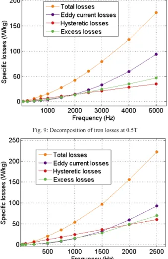
Then, the comparison between the different types of losses is proposed in Fig. 9, Fig. 10 and Fig.11.

The hysteretic losses (energy per m3 _{multiplied by the}

corresponding frequency and divided by the density) appear to be linear. They are an important part of total losses at low frequencies.

Eddy current losses have a huge impact on total losses but they are estimated with the quadratic formula (1). The higher the frequency, the more the eddy currents are preponderant in iron losses. The estimation of eddy current losses is less accurate at high frequency with the formulation, but remains a simple tool to understand the evolution of total losses.

Excess losses are determined by extracting eddy current losses and hysteretic losses from total losses. They are the link between low frequencies (Hysteresis losses) and high frequencies (Eddy current losses). The issue of regulation avoids a proper analysis for high level of B. Nevertheless, the general behavior seems to be the same in for 0.5T, 1T and 1.4T.

Fig. 9: Decomposition of iron losses at 0.5T

Fig.10: Decomposition of iron losses at 1T

Fig. 11: Decomposition of iron losses at 1.4T

V. CONCLUSION

Frequency has a huge impact on iron losses and general magnetic properties of ferromagnetic materials. It determines the composition of iron losses. At high frequency, eddy current losses are dominating whereas at low frequency, hysteretic losses are determining. The excess losses, also called anomalous losses by Bertotti [6], appear as a link between those two ranges of frequency.

Moreover, a regulation issue appears at specific frequencies: an important gap was observed for maximum magnetic field and so coercive field and iron losses. Investigations were proposed. They provide arguments for a dysfunction of device regulation. Indeed, the device did not reach the ordered value of B after the gap frequency whereas it displayed it. That dysfunction could be related to a mechanical vibration according to the measurements made of a stack of sheets or for another material. All those issues highlight the amount of difficulties that represents magnetic measurement. Magnetic measurement results have to be analyzed with caution.

The swelling-up of hysteresis loop with frequency was studied and observed. However, the quantification of hysteresis shape modification with frequency has to be improved in order to take dynamic effect into account in a quasi-static model of hysteresis [7]. Combined with an accurate model of eddy current, a complete model of hysteresis in electrical steel sheet will be determined.

REFERENCES

[1] C. P. Steinmetz, "On the law of hysteresis (part.III) and theory of ferric inductances”, presented at Eleventh General Meeting of the American Institute of Electrical Engineers, Philadelphia, May 18th, 1894. [2] Andreas Krings and Oskar Wallmark,”PWM Influence on the Iron

Losses and Characteristics of a Slotless Permanent-Magnet Motor With SiFe and NiFe Stator Cores”, IEEE Transactions of industry

applications, vol. 51, no. 2, pp. 1475-1484 Apr. 2015

[3] R.Pohl, “Medium-frequency magnetization of steel sheet: the interdependence of hysteresis, eddy currents and magnetic utilization”,

Journal of the Institution of Electrical Engineers - Part II: Power Engineering,Volume: 94, Issue: 38, April 1947.

[4] R. Sato Turtelli, S. Hartl, R. Grössinger, R. Wöhrnschimmel, D. Horwatitsch, F. Spieckermann, G. Polt, and M. Zehetbauer, “Hysteresis and Loss Measurements on the Plastically Deformed Fe–(3 wt%)Si Under Sinusoidal and Triangular External Field”, IEEE Transactions on

magnetics, Vol. 52, NO. 5, May 2016

[5] K. Sun, Y. Yang, Y. Liu, Z. Yu, Y. Zeng, W. Tong, X. Jiang, Z. Lan, R. Guo, and C. Wu, ”Ferromagnetic Resonance Study on Si/NiO/NiFe Films”, IEEE Transactions on magnetics, Vol. 51, No. 11, Nov 2015 [6] G.Bertotti,”General properties of power loss in soft ferromagnetic

materials”, IEEE Transactions on magnetics, vol.24, no.1, pp. 621-630 Jan. 1988.

[7] A.Giraud, A.Bernot, Y. Lefèvre, J.-F. Llibre, " Modeling quasi-static magnetic hysteresis: a new implementation of the play model based on experimental asymmetrical B(H) loops" presented at International Conference on Electrical Machines (ICEM), Lausanne, Switzerland, 2016.