O
pen
A
rchive
T
OULOUSE
A
rchive
O
uverte (
OATAO
)
OATAO is an open access repository that collects the work of Toulouse researchers and
makes it freely available over the web where possible.
This is an author-deposited version published in :
http://oatao.univ-toulouse.fr/
Eprints ID : 15233
The contribution was presented at MAMECTIS 2014:
http://wseas.org/cms.action?id=7764
To cite this version :
Martin, Julien and Georgé, Jean-Pierre and Gleizes,
Marie-Pierre and Meunier, Mickaël Autonomous Pareto Front Scanning using a
Multi-Agent System for Multidisciplinary Optimization. (2015) In: 16th International
Conference on Mathematical Methods, Computational Techniques and
Intelligent Systems (MAMECTIS 2014), 30 October 2014 - 1 November 2014
(Lisbonne, Portugal).
Any correspondence concerning this service should be sent to the repository
administrator:
[email protected]
Autonomous Pareto Front Scanning using a Multi-Agent System for
Multidisciplinary Optimization
J. Martin, J.-P. Georg´e, M.-P. Gleizes IRIT, University of Toulouse 118 Route de Narbonne, Toulouse
FRANCE
{martin, george, gleizes}@irit.fr
Micka¨el Meunier SNECMA Villaroche Rond Point Ren´e Ravaud - R´eau
77550 Moissy-Cramayel FRANCE
Abstract: Multidisciplinary Design Optimization (MDO) problems can have a unique objective or be multi-objective. In this paper, we are interested in MDO problems having at least two conflicting objectives. This characteristic ensures the existence of a set of compromise solutions called Pareto front. We treat those MDO problems like Multi-Objective Optimization (MOO) problems. Actual MOO methods suffer from certain limita-tions, especially the necessity for their users to adjust various parameters. These adjustments can be challenging, requiering both disciplinary and optimization knowledge. We propose the use of the Adaptive Multi-Agent Sys-tems technology in order to automatise the Pareto front obtention. ParetOMAS (Pareto Optimization Multi-Agent System) is designed to scan Pareto fronts efficiently, autonomously or interactively. Evaluations on several aca-demic and industrial test cases are provided to validate our approach.
Key–Words:Pareto Front, Adaptive Multi-Agent System, Multi-Objective Optimization
1
Introduction
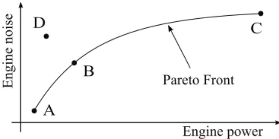
MDO (Multidisciplinary Design Optimization) prob-lems, as their name indicate, intricate several disci-plines in the same problem, each bringing into it its own objectives and constraints. It can be, for instance, the design of a car engine, where we want to maximize the power (mechanics), while minimising the noise (acoustics). Let us call this problem p1. MDO prob-lems are not necessarily multi-objective. We can for instance remove the acoustic objective but still keep the corresponding discipline present (variables, cal-culating models). This reformulated problem has a unique optimal solution, the one that maximizes the power. But MDO problems that have at least two con-tradictory objectives possibly admit an infinity of so-lutions, each solution being a compromise in the ob-jective search space. This is the case of p1, illustrated in figure 1. A and C are extrema solutions. Solution point A represents the most silent engine possible but also the least powerful. On the contrary, C represents the most powerful but also the most noisy. The set of points between them are compromises of these two objectives, such as the point B.
In general, obtaining the complete set of these so-lutions is costly in MOO (Multi-Objective optimiza-tion) [6, 19] as it is necessary to discover and filter, among a cloud of solutions, those that are part of the Pareto front. There is a real need in industry for
meth-A B C Engine power E ngi ne noi se Pareto Front D
Figure 1: Illustration of the p1 problem ods enabling to reduce the cost of these calculations. Indeed, being able to provide the user with the set of compromise solutions in a reasonable delay allows him to rapidly select those that correspond to his cur-rent needs. Automatically obtaining this set of solu-tions in an efficient way is the scientific challenge of our study.
We are going to present how MOO problems are formulated, followed by two notions in relation with the Pareto concept.
1.1
MOO Problem Formulation
A MOO problem is written under the following form: Minimize f(x) = (f1(x), . . . , fp(x)) Subject to gi(x) ≤ 0, i = 1, . . . , m
A MOO problem is constitued by variables, a number p of objective functions f (p≥ 2) and a num-ber m of constraint functions g. Any of these func-tions can be non linear, eventually everyone [10]. The objectives can be dependent or independent, and are often difficult to compare (a cost and a duration for instance).
1.2
Pareto Optimality
Using the formulation of equation 1, here is how are mathematically defined two key Pareto concepts [1]. Definition 1 (Dominance in the Pareto sense) Let
us consider a MOO problem with p minimization objectives. Let u=(u1,. . . ,up) and v=(v1,. . . ,vp) be
two vectors of the values of the objectives for two different solutions. It is said that u dominates v in the sense of Pareto when and only when
∀i ∈ {1, ..., p}, ui ≤ vi∧ ∃j ∈ {1, ..., p} : uj < vj The solution point v is dominated by u as there is no objective for which v is better. If we refer to problem p1 illustrated in figure 1, B dominated D. The solution point D represents an engine both more noisy and less powerful than the solution point B. Definition 2 (Pareto optimality) A solution xu is said to be Pareto optimal if and only of there is no solution xvfor which
v= f (xv) = (v1, ..., vp)
dominates u= f (xu) = (u1, ..., up) As can be seen again in problem p1 in figure 1, D is not a Pareto optimal solution as it is dominated by B for instance. The set of Pareto optimal solutions are the non dominated solutions [9]. Graphically, in the objective space, this set forms the Pareto front.
The following section (2) discusses existing MOO problem solving methods. The multi-agent system dedicated to the autonomous scanning of the Pareto front is described in section 3 and the results in section 4. Finally, section 5 presents ongoing work.
2
Existing Methods
There is a huge diversity of methods for treating MOO problems. In this part, we will present the two most used groups of methods, namely the ”classical” meth-ods and the ”intelligent” methmeth-ods. After a rapid anal-ysis of their strengths and weaknesses, we will justify the use of an Adaptive Multi-Agent System to solve these kind of problems.
2.1
Classical Methods
Classical methods concentrate on the transformation of the MOO problem in a mono-objective problem, so as to be able to use a mono-solution solver. There are several manners to do this transformation. We can ag-gregate the objective functions in one function. We can also keep only one objective function and trans-form the others into constraints. The resulting prlem admits a unique solution (as there is only one ob-jective). If we want other solutions on the Pareto front using these techniques, it is necessary to execute them several times, modifying the formulation each time, changing how the transformation of an MOO problem into a mono-objective problem is done. For instance, it can be the tuning of the weighting inside the aggre-gation function.
2.1.1 The Weighted Sum Method
The weighted sum method transforms the MOO prob-lem into an mono-objective probprob-lem in the following way:
• attribution of a weight wj for each objective function, a weight representing the relative im-portance for each objective fj in obtaining a so-lution [18],
• sum of everything,
• minimization of this sum with a mono-solution solver. Minimize Z= p X j=1 wjfj(~x) with wj ≥ 0 and p X j=1 wj = 1 (2)
To find Pareto optimal solutions using this method, the user needs to choose a set of weights, find the first solution, modify the weights, relaunch the mono-objective solving and so on. Without ex-pert knowledge of the problem, the choice of these weights wj can be quite hard. Moreover, if some ob-jective functions are non linear, a modification of a weights does not guarantee a different solution. It is also impossible to find solution points in the concave zones of the front with this method [15]. Finally, it is hard to control the repartition diversity of the solution points in the objective space [18, 4]. Work to enhance this method has been proposed [11, 15]. Neverthe-less, specific parameters of these algorithms need to be correctly initialised to obtain satisfactory results.
2.1.2 The ε-Constraint Method
This method has been created so as to find the Pareto front by optimising only one objective and treating the others as constraints. Similar to the weighted sum methods, the front is obtained by repeatedly using the method, the user being required to modify the con-straint bounds between each execution. By notingΩ for the decision space, this method is formalised as:
Minimize fk(~x), ~x ∈ Ω
with fi(~x) ≤ εiand gj(~x) ≤ 0 i= 1, 2, . . . , p ; i 6= k
j= 1, 2, . . . , m
(3)
This is again a simple technique to implement, but very costly in calculation time, especially as there is no guarantee that the obtained solutions are globally Pareto optimal [16, 4].
We are here limited to the presentation of the two most popular classical approaches. There are others such as the Benson method [2], goal-programming [3], interactive methods such as iMOODs [20] and NIMBUS [14]. . .
These approaches show their limits as soon as the user wants to extract the Pareto optimal solutions in their entirety:
• The majority of them can at best find a unique Pareto optimal solution point for each execution. To find several, the algorithm needs to be exe-cuted several times, without any guarantee con-cerning the diversity of the points in regard to the objective space.
• Some of these approaches are incapable of find-ing solutions in the zones where the Pareto front is non convex, as is the case for the weighted sum method. Some research was done to fix this [15], but only for problems with two objectives, the scaling up still needs to be demonstrated. • All these approaches require user information,
on which depend the quality of the solutions. These are the weights for the pondered sum method or the bounds for the ε-contraint method. The choice of those informations is generally dif-ficult and requires from the user expert knowl-edge on the application domain or the algorithm, or even both.
The intelligent approaches appeared to tackle these problems. They are part of the a posteriori ap-proaches, for which the user intervenes afterwards the solving to choose the solution point.
2.2
The intelligent methods
Contrary to the classical approaches, these methods try to generate the Pareto front by considering each objective as it is. Progress in calculation power and the development of population based algorithms con-tributed to their emergence. One of the advantages over classical methods is that they manage to evalu-ate several solutions at each iteration. Moreover, they bring a greater ease of use, particularly when no a
priori knowledge is available, which is the case for most real-world industrial problems. The evolution-ary methods are part of the intelligent methods [5]. They simulate a biological process of evolution in a population of candidate solutions so as to guide them towards the Pareto front. These solutions are sub-jected to mutation and crossing operations, produc-ing a new generation of solutions at each iteration, and only a set of the best are kept during execution. The difficulty is to manage to guide them towards the front while guaranteeing the repartition diversity on the whole front. The evolutionary methods regroup genetic algorithms, evolutionary algorithms, as well as evolution strategies. These three categories differ on the way the solutions are evaluated as well as on the mutation and crossing operators they use. To illustrate the intelligent methods, we are going to present the NSGA genetic algorithm, which has the particularity to directly integrate Pareto concepts in its functioning. 2.2.1 Non-Dominated Sorting Genetic Algorithm
(NSGA)
NSGA is a genetic algorithm based on the idea pro-posed by Goldberg to sort the solutions by their dominance ranking in the Pareto sense [7]. Srini-vas and Deb used Goldberg’s work and implemented NSGA [17] so as to use the non dominance rank to evaluate the quality of the solutions: the less there exists solutions dominating s1 among the candidate population, the more favourably s1 is evaluated.
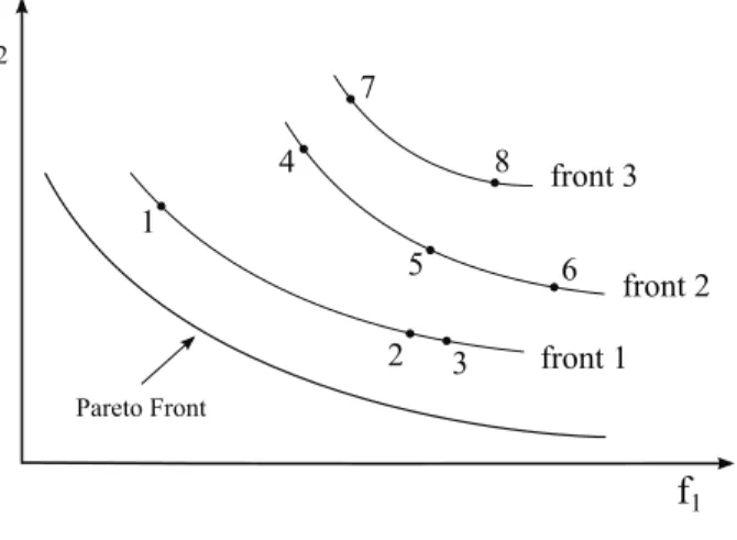
To run a genetic algorithm, it is necessary to have an initial solution population. We are going to sim-ulate the execution of NSGA starting from the popu-lation illustrated in figure 2. The initial popupopu-lation is composed of 8 solutions. The Pareto front is also rep-resented. An iteration of NSGA is composed of the following phases:
• sorting of the solutions based on their non domi-nance rank,
• use of this information in the application of the evaluation function,
• selection, mutation and crossing (3 common op-erations in genetic algorithms).
First, the algorithm sorts the whole population de-pending on their non dominance rank. No solution dominates points 1, 2 and 3, and so they constitute front 1. The algorithm will now ignore points 1, 2, 3 and find the new non dominated solution : 4, 5 and 6 (front 2). Front 3, composed by solutions 7 and 8 is determined using the same manner. We obtain mutu-ally exclusive solution classes, each class being con-tained in a distinct front, as illustrated in figure 2.
f
2f
1 1 2 3 4 5 6 7 8 front 1 front 2 front 3 Pareto FrontFigure 2: The different front ranks
After this sorting phase, NSGA evaluates the so-lutions. This algorithm favours the solutions which are nearer to the Pareto front, so it is important to note that any solution in a front ranked n will have a lower score that one from a front ranked n-1, and this in a transitive manner. In a second time, NSGA will diminish the score of the solutions depending of the number of other solutions in their neighbourhood. This choice from Srinivas and Deb is related to the work of Goldberg and Richardson [8] who proposed to degrade the score of similar solution rather than merge them. The user have to choose the parameters for calculating the neighbourhood. It has been shown that the performance of NSGA are impacted by this choice [17].
These methods require, as with the classical methods, to fix specific parameters required for the functioning (neighbourhood, but also population size, selection, mutation and crossover rates, etc.). More-over, calculation costs increase enormously with the increase in the number of objectives and population size. The aim of the use of an Adaptive Multi-Agent System to obtain the Pareto front is to remove the need for algorithm parameters, these systems being able to learn during the solving. Moreover, the multi-agent system, by taking control of an underlying solver with a set of specific characteristics, is able to move along the Pareto front and scan for new solutions in an
au-tonomous and efficient way.
3
The ParetOMAS system
The algorithm scanning the Pareto front is consti-tuted by an Adaptive Multi-Agent System we call
ParetOMAS (Pareto Optimization Multi-Agent Sys-tem). This system makes use of an underlying mono-solution solver1 that it will control so as to automat-ically build the Pareto front of any given problem, without the need of human intervention (but allowing interaction if convenient).
Graphical tools have been developed so as to vi-sualize the Pareto front building as it is occurring in the objective space. ParetOMAS allows interaction: the user can at any time request a search direction for the following solutions. The user can also modify its preferences concerning solution precision as well as solution spacing. ParetOMAS is able to take into ac-count these changes during execution.
As a result, the underlying solver needs to satisfy specific criteria:
• being able to signal that it has converged under a given precision,
• being able to bestow more or less importance to objectives during the solving,
• being able to accept the modification of the de-scription of a problem, for instance the transfor-mation of a minimization in a maximization ob-jective, during solving.
During the ID4CS2 project, a mono-solution multi-agent system solver has been developed [13, 12]. It constitutes a solver compatible with Pare-tOMAS and will be used to obtain the results pre-sented in section 4.
ParetOMAS can be activated or deactivated at any time by the user without stopping the solver. Fig-ure 3 represents the interaction diagram between Pare-tOMAS, the solver and the user.
When it is activated, its role is to efficiently ori-ent the search of new solution points in the objective space, so as to obtain a solution set constituting the Pareto front, in accord with the preferences of the user concerning precision, distribution, number of points, etc. The solver finds a solution point, ParetOMAS detects this and sends a new request to the solver so that it can find a new solution point. The coupled sys-tem{ParetOMAS, solver} constitutes a new adaptive multi-solution solver.
1
Solver that provides a unique solution, in opposition to a solver that provides a set of solutions
ParetoSolution
agents
notifications preferences observation interactionsUser
ParetoGuide
agent
Solver
prefere ncesParetOMAS
Figure 3: Interaction diagram of ParetOMAS
ParetOMAS is composed of two types of agents: a ParetoGuide agent and ParetoSolutions agents. The user has access to a dedicated interface to input its preferences (distance between solution points, choice of a search direction . . . ). The two following sub-sections present the roles of these two agent types, describe their behaviour, interaction and life-cycle.
3.1
The ParetoGuide Agent
The ParetoGuide agent constitutes an interaction hub between the user, the solver and the ParetoSolution agent. There is only one ParetoGuide per instance of ParetOMAS. Its role is to take into account the pref-erences of the user and those of the ParetoSolution agents during execution. Its nominal behaviour is de-scribed by the algorithm 1. Each time a solution point is found by the solver, ParetoGuide creates a Pare-toSolution agent representing this new point.
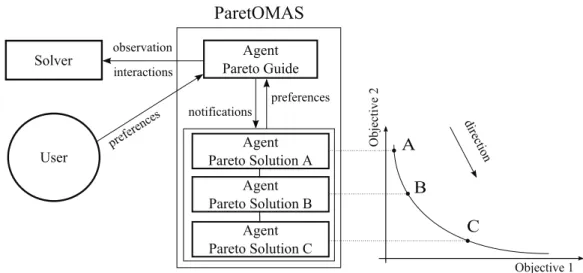
The user can inform the system of a direction preference for the scanning of the front. The Pare-toSolution agents can do the same. If the user is mak-ing a choice, ParetoGuide ignores the requests from the ParetoSolutions agents and takes into account the one from the user. If this is the case but there is an im-possibility (boundaries of the problem for instance), ParetoGuide then defaults on the preferences of the ParetoSolution agents while signalling to the user why it could not comply. In any case, ParetoGuide then sends a corresponding request to the solver so that it is able to find a new solution in the chosen direction. This behaviour is illustrated in figure 4.
3.2
The ParetoSolution Agents
The role of the ParetoSolution agents is to orient Pare-toGuide in the objective space so as to obtain an effi-cient scanning and a relevant resulting front. These
if Solver has found a solution then Creation of a ParetoSolution agent; if User is forcing a direction then
Send a request to the solver favouring this direction;
else
Inquire of direction preferences from the ParetoSolution agents;
Send a request to the solver favouring this direction;
end end
Algorithm 1: Nominal behaviour of the ParetoGuide agent
agents are created dynamically by ParetoGuide as de-scribed previously. Each ParetoSolution agent pos-sesses, in the objective space, a neighbourhood of other ParetoSolution agents. This neighbourhood is defined, for each ParetoSolution agent, by the set of ParetoSolution agents being located at or under a eu-clidean distance d, defined by the user (as it will rep-resent the structure of the front at the end)3.
A ParetoSolution agent sends requests to Pare-toGuide so as to obtain a neighbourhood that satisfies it. This is translated by ParetoGuide into a direction in which to scan the objective space. The user, by diminishing d, increases the sampling of the Pareto front, and the other way round. d can be modified any time during execution. A ParetoSolution agent can also send a request to be ”shifted” in the objective space so as to enhance the homogeneity of the sam-pling (if the user wants a perfect ”grid” as a Pareto plan for instance).
Information given to a ParetoSolution agent at creation are:
• its coordinates in the objective space,
• the state of the corresponding input variables, • the objective values initially aimed at by
Pare-toGuide,
• the calculation time needed to obtain this solu-tion,
• its neighbourhood of ParetoSolution agents (pos-sibly empty),
• the calculation time of the neighbourhood. Each time a new ParetoSolution agent is created, it notifies the agents situated in its neighbourhood for
3It can be noted that contrary to the evolutionary methods, this
Agent Pareto Solution A notifications preferences observation interactions User Agent Pareto Guide Solver prefere nces
ParetOMAS
A
B
C
Objective 1 Obj ec ti ve 2 di re ction Agent Pareto Solution B Agent Pareto Solution CFigure 4: ParetOMAS during execution, three solutions points have been found
them to update their knowledge. It then adopts a nom-inal behaviour as described in algorithm 2.
if Unsatisfactory neighbourhood then
Send a request to ParetoGuide for a chosen
searchdirection;
else if Non homogeneous placement then Send a request to ParetoGuide for a chosen
shiftdirection end
Algorithm 2: Nominal behaviour of the ParetoSolu-tion agents
4
Implementation And Feasibility
Proof
ParetOMAS is currently in a prototype state. The user is provided with a temporary graphical interface for him to input its preferences, such as the distance be-tween solution points and optional search direction preferences. The Pareto front scanning is observable in real time for problem with two or three objectives. ParetOMAS has been tested on continuous and dis-continuous Pareto fronts.
4.1
Continuous Pareto Front
The test case we show here admits a continuous Pareto front. It is a topology for which the ParetOMAS agents have the simplest behaviours.
4.1.1 TurboFan
This test case is provided by Snecma4as a study case. The goal is to optimise output parameters of a classic double flux turbo-reactor (civil plane engine) as illus-trated in figure 5. This problem uses thermodynamic models. The two output parameters to optimise are the consumption s which needs to be minimized and the thrust T dm0 which needs to be maximized, both being contradictory. The two input variables are the dilution rate bpr and the pressure ratio pic. The dilu-tion rate represents the ratio between the air volume aspirated by the blower and the air volume reaching the low pressure compressor. The pressure ratio is the ration between the pressure produced by the compres-sors and the initial pressure of the environment. bpr and piceach have their validity range and we want to obtain all the couples of compromise solutions.
The results obtained by ParetOMAS are seen in figure 6. The space between the solution points can be chosen by the user and an arbitrary value has been used here. This problem is well known by Snecma and the documentation indicates that all the Pareto front points have in fact as a corresponding input value the variable pic at 40, and any value of bpr then gives a Pareto optimal solution. This is verified by the solu-tion found by ParetOMAS. Figure 7 superposes these solutions with a graphical representation of the front obtained by exhaustive calculation (fixing pic at 40 and adjusting bpr over its complete range).
4.2
Discontinuous Pareto Front
The two following test cases present a discontinuous Pareto front. This induces a risk that the solver used
4
Figure 5: A TurboFan Engine (CC BY-SA K. Aain-sqatsi)
Figure 6: The set of solutions proposed by Pare-tOMAS for the TurboFan problem
by ParetOMAS stops in a local minimum. This situa-tion requires a secondary behaviour for ParetoGuide, enabling it to guide the solver out of a local minima. This exploration mechanism will be explained and re-sults will be shown for a problem with two objectives and one with three objectives.
4.2.1 A problem With Two Objectives
This problem has been artificially generated to con-front ParetOMAS to two contradictory objectives with a discontinuous Pareto front. The problem is consti-tuted by a unique calculation model that describes the topology of the front. This model has two input vari-ables x and y, and two output varivari-ables X and Y that require minimization:
Figure 7: Superposition of the real Pareto front with the points obtained by ParetOMAS on the TurboFan problem
X = x
Y = 1x+ 50(x−.2)(x−.2)+130 +40(x−.6)(x−.6)+120 + y2 The output Y is the sum of 4 functions:
• h(x) = x1
• k(x) = 50(x−.2)(x−.2)+130 • t(x) = 40(x−.6)(x−.6)+120 • w(x) = y2
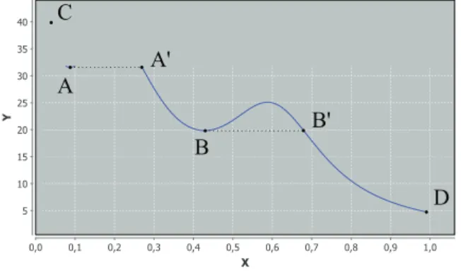
The sum of h, k and t results in a non-monotonous function, illustrated figure 8, which ad-mits 2 local minima, A and B. Finaly, function w is added to make the search space above h(x) + k(x) + t(x) admissible. The Pareto optimal solutions of this problem are situated on the curve described by h(x) + k(x) + t(x).
Figure 9 shows the solutions obtained by Pare-tOMAS. Initial values of the input variables have been chosen such that the first discovered solution point is C on figure 8. The objective Y is favoured compared to objective X, thus the scanning direction goes from left to right. ParetOMAS discovers the solutions be-tween points C and A. When it arrives at A, the solver is blocked in a local minimum: it is not possible, lo-cally, to improve Y by following the curve. Pare-tOMAS, by a decision of ParetoGuide commutes to an
explorationmode to extract the system from the local minimum. For this ParetoGuide temporarily redefines the problem:
• recording of the value of the objective that was initially favoured,
A B A' B' C D Figure 8: X = x and Y = h(x) + k(x) + t(x) • inversion of the nature of the other objective
(minimization becomes maximization, and the other way round),
• inversion of the favouring of objectives,
• surveillance of the evolution each new point cal-culated by the solver so as to detect the moment when the value of the objective that was initially favoured becomes better than the value recorded before exploration,
• reformulation back to the initial problem. This is how it is translated when the system ar-rives at point A. The favoured objective is Y , Pare-toGuide records its value (31.55). X and Y have both minimization objectives. The objective on X becomes a maximization objective and becomes the favoured objective. The minimization objective on Y , while not favoured compared to X, is still maintained so that the solver, by taking it into account, tends to-wards the curve. The problem is temporarily trans-formed and has a unique solution at point D. Visually, we can see that the current working point moves from A to A’ while staying stuck to the curve. When this point oversteps A’, ParetoGuide detects that the value of Y becomes better than when it was at point A and switches back to the initial formulation of the prlem. The objective on X becomes a minimization ob-jective again and the obob-jective on Y is favoured again for the solving. ParetOMAS then discovers the solu-tions between A’ and B, and is blocked again in a local minimum. Commuting again in exploration mode, it finds the solutions between B’ and D.
The solutions discovered by ParetOMAS are vis-ible on figure 9. Figure 10 superposes these solution to the function h(x) + k(x) + t(x) responsible for the topology of the front. For each point proposed, we can verify that input variable y is equal to zero, which shows that the point is indeed on the front and by com-paring Y that it is a Pareto optimal solution.
Figure 9: Solutions obtained on the non-monotonous problem with 2 objectives
Figure 10: Superposition of the obtained solutions with the real curve on which the front is located (the two ”hills” are not part of the front)
4.2.2 A Problem With Three Objectives
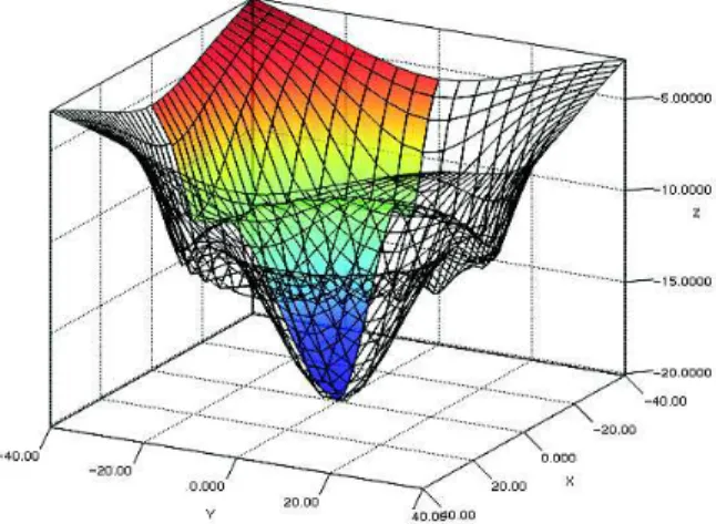
This problem has been artificially generated in the same spirit as the previous. But this time there are three objectives, the front is a surface (Pareto plan). The problem has a unique calculation model respon-sible for the topology of the front, takes three input variables x, y and z, as well as three output variables X, Y and Z requiring minimization:
X = x Y = y Z = −20 0.002(x2+y2)+1− 5 0.05(√x2+y2−30)(√x2+y2−30)+1+ z 2
output Z is the sum of 3 functions: • q(x, y) = −20
• r(x, y) = − 5
0.05√x2+y2−30)(√x2+y2−30)+1
• c(z) = z2
q(x, y)+r(x, y) is represented in figure 11. Those two functions have been chosen so as to create a sort of basin with an infinity of local minima, enabling the testing of the exploration mode on 3 objectives.
Figure 11: q(x, y) + r(x, y)
Function c is added to make the search space above q(x, y) + r(x, y) admissible. The Pareto optimal solutions of this problem are illustrated figure 12 : it is the colored region of the surface.
Figure 12: Pareto optimal solutions
The solutions discovered by ParetOMAS are visi-ble on figure 13. For each point proposed, we can ver-ify that input variable z is equal to zero, which shows that the point is indeed on the Pareto front.
5
Ongoing Works
ParetoGuide Behavior Refinement The
ParetoGu-Figure 13: Solutions obtained on the three objectives problem
ide behavior is continuously updated in order to optimize its operation with the ID4CS solver. The most challenging part of this work is the translation of the user and ParetoSolutions directions preferences into something understandable by ID4CS. Our ap-proach is generic and would work with compatible solver. We work on a generic communication protocol between ParetOMAS and the solver.
ParetoSolution Agents The behavior of those agents described in subsection 3.2 is not totally implemented. Those agents don’t use all the informa-tions they have and so are currently suboptimal. The precision toward the prefered directions they send to ParetoGuide will improve with their refinement, making ParetOMAS more effective.
Problems Generator In order to validate our approach, a problems generator is developed. The objective is to be able to automatically generate a great number of problems having various topologies (continuous, discontinuous, convexe, concave...). A metrics system allowing the automatic evaluation of the obtained solutions is also developed (calculation time, distance from the pareto front, homogeneous distribution...).
Academic benchmarks comparison We are reviewing academic benchmarks in order to compare our approach with other optimization methods.
Real-World Industrial Problems ParetOMAS will be tested on real-world industrial problems with SNECMA problems. This will validate the scalability of ParetOMAS with problems having 4 or more
objectives.
Acknowledgements: We want to thank Snecma and the french National Association for Research and Technology for financing this work.
References:
[1] A. Ben-Tal. Characterization of pareto and lex-icographic optimal solutions. In G. Fandel and T. Gal, editors, Multiple Criteria Decision
Mak-ing Theory and Application, volume 177 of
Lec-ture Notes in Economics and Mathematical Sys-tems, pages 1–11. Springer Berlin Heidelberg, 1980.
[2] H. Benson. Existence of efficient solutions for vector maximization problems. Journal of
Op-timization Theory and Applications, 26(4):569– 580, 1978.
[3] A. Charnes and W. Cooper. Goal program-ming and multiple objective optimizations: Part 1. European Journal of Operational Research, 1(1):39 – 54, 1977.
[4] C. A. C. Coello. A comprehensive survey of evolutionary-based multiobjective optimization techniques. Knowledge and Information sys-tems, 1(3):269–308, 1999.
[5] K. Deb. Multi-objective optimization using
evo-lutionary algorithms, volume 16. John Wiley & Sons, 2001.
[6] J. Dr´eo, A. P´etrowski, P. Siarry, and E. Taillard.
Metaheuristics for Hard Optimization: Methods and Case Studies. Springer, 2006.
[7] D. E. Goldberg et al. Genetic algorithms in search, optimization, and machine learning, vol-ume 412. Addison-wesley Reading Menlo Park, 1989.
[8] D. E. Goldberg and J. Richardson. Genetic algo-rithms with sharing for multimodal function op-timization. In Genetic algorithms and their
ap-plications: Proceedings of the Second Interna-tional Conference on Genetic Algorithms, pages 41–49. Hillsdale, NJ: Lawrence Erlbaum, 1987. [9] J. Horn. Multicriterion decision making. In
T. Back, D. B. Fogel, and Z. Michalewicz, ed-itors, Handbook of Evolutionary Computation. IOP Publishing Ltd., Bristol, UK, UK, 1st edi-tion, 1997.
[10] C. L. Hwang, A. S. M. Masud, et al. Multiple
objective decision making-methods and applica-tions, volume 164. Springer, 1979.
[11] Y. Jin, M. Olhofer, and B. Sendhoff. Dynamic weighted aggregation for evolutionary multi-objective optimization: Why does it work and how?, 2001.
[12] T. Jorquera. An adaptive multi-agent system for self-organizing continuous optimization. Phd thesis, University of Toulouse, Toulouse, France, septembre 2013.
[13] T. Jorquera, J.-P. Georg´e, M.-P. Gleizes, and C. R´egis. A Natural Formalism and a Mul-tiAgent Algorithm for Integrative Multidisci-plinary Design Optimization (regular paper). In IEEE/WIC/ACM International Conference
on Intelligent Agent Technology (IAT), Atlanta, USA, 17/11/2013-20/11/2013, page (on line), http://www.computer.org, 2013. IEEE Computer Society.
[14] M. M. M. Kaisa Miettinen. Interactive multiob-jective optimization system www-nimbus on the internet. Computers and Operations Research, 27(7-8):709–723, 2000.
[15] I. Kim and O. de Weck. Adaptive weighted-sum method for bi-objective optimization: Pareto front generation. Structural and Multidisci-plinary Optimization, 29(2):149–158, 2005. [16] U. Nangia, N. Jain, and C. Wadhwa. Surrogate
worth trade-off technique for multi-objective op-timal power flows. In Generation,
Transmis-sion and Distribution, IEE Proceedings-, vol-ume 144, pages 547–553. IET, 1997.
[17] N. Srinivas and K. Deb. Muiltiobjective op-timization using nondominated sorting in ge-netic algorithms. Evolutionary computation, 2(3):221–248, 1994.
[18] M. T. Tabucanon. Multiple criteria decision making in industry. Elsevier Amsterdam, 1988. [19] E.-G. Talbi. Metaheuristics - From Design to
Implementation. Wiley, 2009.
[20] R. Tappeta, J. Renaud, and J. Rodr´ıguez. An interactive multiobjective optimization design strategy for decision based multidisciplinary de-sign. Engineering Optimization, 34(5):523–544, 2002.