© Mohammad Pousti, 2019
Linear scanning ATR-FTIR for mapping and high
throughput studies of bacterial biofilms in microfluidic
channels
Thèse
Mohammad Pousti
Doctorat en chimie
Philosophiæ doctor (Ph. D.)
Québec, Canada
Linear scanning ATR-FTIR for mapping and high
throughput studies of bacterial biofilms in
microfluidic channels
Thèse
Mohammad Pousti
Sous la direction de :
iii
Résumé
Le domaine de la chimie bioanalytique est en plein développement. Les tendances vers une caractérisation plus précise, une analyse à haut débit et une automatisation accrue offrent la promesse de systèmes capables de fournir des informations plus détaillées sur les systèmes biologiques vivants. Les biofilms sont répandus dans la plupart des écosystèmes. Ils peuvent être formés par la plupart des microorganismes. Les biofilms microbiens sont des communautés multicellulaires de bactéries, adhérant à une surface, entourées d'une substance polymère extracellulaire (EPM). En raison de leur origine naturelle, les biofilms bactériens sont de plus en plus étudiés et utilisés pour des applications en biocatalyse, en auto-guérison et en tant que systèmes pouvant fonctionner efficacement dans des conditions ambiantes. Les principaux facteurs qui contrôlent le développement du biofilm et ses propriétés matures sont les conditions hydrodynamiques appliquées et les concentrations en éléments nutritifs. Les propriétés mécaniques du système EPM peuvent être personnalisées en fonction de son environnement. De plus, l’existence de différents groupes chimiques fonctionnels dans le biofilm permet de piéger des molécules organiques et des ions dissous.
Cette thèse porte sur le développement d'une technique permettant une flexibilité et une précision dans la croissance et la détection des biofilms de Pseudomonas sp. Bactérie CT07. Le système analytique est multimodal afin d’obtenir des informations sur les propriétés chimiques et structurelles du biofilm. À cette fin, la microscopie optique et la spectroscopie infrarouge à transformée de Fourier (FTIR) à réflexion totale atténuée (ATR) ont été couplées dans un système analytique coordonné avec des canaux microfluidiques pour contrôler les conditions de croissance des biofilms. Pour atteindre cet objectif, un montage ATR-IR fait maison a été développé pour permettre de sonder différents emplacements au-dessus du cristal d'ATR afin d'ajouter une capacité de mesure au système situé à différents emplacements. Les différentes méthodologies développées dans cette thèse peuvent être appliquées à d'autres systèmes complexes à l'avenir. La combinaison de la microfluidique pour un contrôle de flux précis ainsi que des mesures multiplexées dans un microcanal parallèle est la clé pour obtenir des indices importants et statistiquement pertinents sur la croissance des biofilms et sur les méthodes pour les contrôler.
iv
Abstract
The field of bioanalytical chemistry is currently undergoing rapid development. Trends toward more precise characterization, high-throughput analysis and greater levels of automation collectively offer the promise of systems that can deliver deeper insights into living biological systems. Biofilms are widespread in most ecosystems. They can be formed by most microorganisms. Microbial biofilms are multicellular communities of bacteria, adhering to a surface, surrounded by an extracellular polymeric matrix (EPM). Because they are natural, bacterial biofilms are increasingly being studied and used for applications in biocatalysis, self-healing and as systems that can function effectively under ambient conditions. The main factors controlling biofilm development and its mature properties are the applied hydrodynamic conditions and nutrient concentrations. The mechanical properties of the EPM can be customized based on its environment. Additionally, the existence of different functional chemical groups within biofilm makes it possible to trap organic molecules and dissolved ions.
This PhD thesis focus on developing a system-level technique that enables flexibility and precision in the growth and detection of biofilms from Pseudomonas sp. CT07 bacteria. The analytical system is multi-modal, in order to obtain information on biofilm chemical and structure properties. To this end, optical microscopy and attenuated total reflection (ATR) Fourier transform infrared (FTIR) spectroscopy have been coupled into one coordinated analytical system with microfluidic channels to control the growth conditions of biofilms. To achieve this goal, a home-built ATR-FTIR stage was developed for probing different locations on top of ATR crystal. The methodologies developed in this thesis can be applied to other complex analytical systems in the future. The combination of microfluidics for precise flow control as well as multiplexed measurements in parallel microchannel is the key to obtaining important and statistically relevant clues to the growth of biofilms and the methods to control them.
v
Table of Contents
Résumé ... iii
Abstract ... iv
List of Figures ... x
List of Tables ... xxi
List of Equations ... xxii
List of abbreviations ... xxiii
Acknowledgments ... xxv
Foreword ... xxvi
Introduction ... 1
1. Chapter 1: Literature review ... 3
1.1. Bacteria and their Biofilms ... 3
1.1.1. Biofilm chemical components and importance of early detection... 5
1.1.2. Biofilm measurement ... 6
1.2. Microfluidics ... 6
1.2.1. Pumping mechanism ... 8
1.2.2. Materials for microfluidics ... 10
1.2.3. Microfabrication techniques ... 12
1.3. Microfluidics and biofilms ... 14
1.4. Spectroscopy: chemical measurement of biofilm in microfluidics ... 15
1.4.1. Vibrational spectroscopy ... 15
1.5. Different sampling modes in IR ... 19
1.5.1. Transmission mode ... 19
1.5.2. External reflection mode ... 20
1.5.3. Attenuated total reflection ATR-FTIR spectroscopy ... 21
1.6. Infrared spectroscopy for study of biofilms ... 23
1.7. Compatibility of microfluidics and ATR-FTIR system ... 24
1.7.1. IR technique for studying hydrated biofilms in microchannels ... 24
1.7.2. Advantages of ATR-FTIR for biomaterial sensing ... 25
1.8. Bibliography ... 25
2. Chapter 2: Materials and experimental procedure ... 32
vi
2.1.1. Mask fabrication ... 32
2.1.2. Mould fabrication ... 32
2.1.3. Device fabrication ... 33
2.2. Sealing layer in microfabrication ... 35
2.2.1. Plasma bonding ... 35
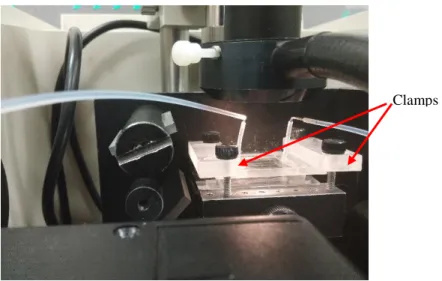
2.2.2. Clamping ... 36
2.3. Flow control ... 36
2.4. Medium preparation ... 37
2.5. Bacteria preparation ... 37
3. Chapter 3: Microfluidic bioanalytical flow cells for biofilm studies: A review ... 38
3.1. Résumé... 39
3.2. Abstract ... 40
3.3. Introduction ... 41
3.3.1. Literature review ... 41
3.3.2. Bacterial biofilms, grand analytical challenges ... 43
3.3.3. Control using microfluidics ... 44
3.4. Microscopy ... 46
3.4.1. Optical microscopy ... 46
3.4.2. Chemical tracers and time-lapse imaging ... 47
3.4.3. High-resolution microscopy ... 48
3.5. Electrochemical measurements ... 52
3.5.1. Two-electrode systems ... 52
3.5.2. Three-electrode systems ... 54
3.6. Spectroscopy and chemical imaging ... 57
3.6.1. Raman spectroscopy ... 58
3.6.2. Infrared spectroscopy... 59
3.7. Other techniques and emerging approaches ... 61
3.7.1. Advanced microscopy ... 61
3.7.2. Electrochemistry ... 62
3.7.3. Spectroscopy ... 63
3.7.4. Mass spectrometry ... 63
3.7.5. Respirometry ... 64
vii
3.9. Bibliography ... 67
4. Chapter 4: 1D-IR scanning system development ... 86
4.1. Technical development of the automatic 1D-IR scanning system ... 86
4.1.1. Overall architecture positioning accuracy of stepper motor ... 86
4.1.2 Overall system synchronization ... 88
4.1.3. Position control over the stepper motor ... 89
4.1.4. Optical imaging and components ... 91
4.1.5. Data acquisition and data treatment with camera ... 93
4.2. IR data acquisition ... 93
4.2.1. ATR imaging accessories ... 94
4.2.2. Automated data acquisition with FTIR ... 94
4.2.3. Data acquisition and data treatment with IR instrument ... 94
4.2.4. Resolution optimization ... 94
4.2.5. Signal intensity from different ATR crystals ... 98
4.2.6. Spatial resolution ... 98
4.3. FTIR and camera alignment ... 100
4.4. Camera measurement development ... 100
4.4.1. Results for changing gain ... 103
4.5. Example Code used in the projects ... 106
4.5.1. Code for gain recognition... 106
4.5.2. Code for overall data acquisition ... 108
4.6. Bibliography ... 110
5. Chapter 5: Linear scanning ATR-FTIR for chemical mapping and high throughput studies of bacterial biofilms in microfluidic channels ... 111
5.1. Résumé... 112
5.2. Abstract ... 113
5.3. Introduction ... 114
5.4. Materials, equipment and methodology ... 116
5.4.1. Infrared spectroscopy ... 116
5.4.2. Microscope imaging ... 116
5.4.3. Microfluidic device fabrication with imbedded ATR crystal probe surface ... 117
5.4.4. Spectral data treatment ... 118
viii
5.4.6. Biofilm cultivation and inoculation ... 118
5.5. Results ... 119
5.5.1. System development ... 119
5.5.2. Determination of spatial resolution and system validation ... 120
5.5.3. Measurements on growing biofilms ... 124
5.5.4. System repeatability in bacterial biofilm measurements ... 126
5.6. Discussion ... 130
5.7. Conclusion ... 132
5.8. Bibliography ... 133
5.9. Supporting Information ... 138
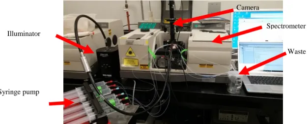
5.9.1. System setup ... 138
5.9.2. Microfluidic device designs ... 141
5.9.3. Overall software flow and graphical user interface ... 142
5.9.4. Imaging brightness ... 146
5.9.5. Technical validation experiments ... 148
6. Chapter 6: Altered biofilm formation at plasma bonded surfaces in microchannels studied by attenuated total reflection infrared spectroscopy ... 150
6.1. Résumé... 151
6.2. Abstract ... 152
6.3. Introduction ... 153
6.4. Experimental ... 154
6.4.1. Materials and equipment ... 154
6.4.3. Biofilm cultivation ... 155
6.4.4. Data acquisition ... 155
6.5. Results and Discussion ... 155
6.6. Conclusion ... 162
6.7. Bibliography ... 162
6.8. Supplementary Materials... 166
6.8.1. Sections ... 166
6.8.2. Dynamic changes to the contamination layer during exposure to pure nutrient solution .... 166
6.8.3. Effect of pressure compression of PDMS channels to Ge ATR surface ... 168
6.8.4. Device interface with ATR-FTIR ... 169
7. Chapter 7: A surface spectroscopy study of a Pseudomonas fluorescens biofilm in the presence of an immobilized air bubble ... 170
ix 7.1. Résumé... 171 7.2. Abstract ... 172 Keywords ... 172 7.3. Introduction ... 173 7.4. Experimental Methods... 174
7.4.1. Microfluidic Device Fabrication ... 174
7.4.2. Biological Preparation ... 175
7.4.3. Acquisition System ... 175
7.4.4. Spectroscopy and Microscopy Acquisition Parameters ... 176
7.5. Results and Discussion ... 177
7.5.1. Optical Microscopy ... 177
7.5.2. Scanning ATR-FTIR... 179
7.5.3. Effect of Bubble on Lipid formation and Biofilm Restructuring ... 184
7.5.4. Analysis of Protein Absorbance Band Position ... 186
7.6. Conclusion ... 187
7.7. Bibliography ... 188
8. Chapter 8: Perspective and future works ... 193
x
List of Figures
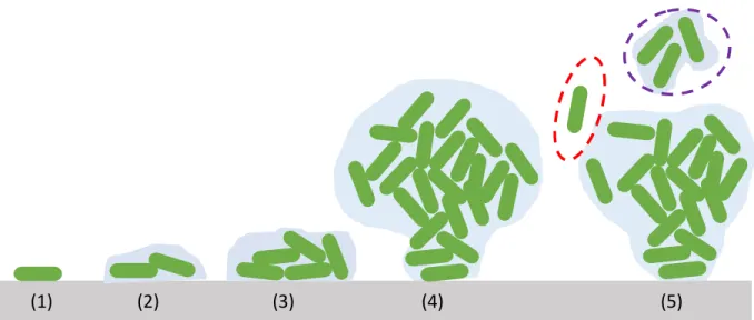
Figure 1.1. Depiction of typical stages of biofilm formation. (1) Transport and initial attachment of microbes to a molecular conditioning layer, (2) irreversible adhesion or attachment mediated by small amounts of EPM (blue), (3) formation of microcolonies and continued accumulation of EPM, (4) thickening and structuration of the biofilm and (5) detachment and dispersion of the cells
individually (red dashed) or in clumps known as flocs (purple dashed). ...4
Figure 1.2. (a ) Schematic diagram of the Michelson interferometer. (b) An example of a raw measured interferogram (c) and corresponding single beam spectrum after fast Fourier transformation. ...18
Figure 1.3. Schematic representation of transmission mode ...20
Figure 1.4. Schematic diagram of the external reflection measurement ...21
Figure 1.5. Two different types of ATR crystals, (a) Single bounce crystal that specially used for highly absorbing samples and/or relatively low index of refraction ATR materials. b) Multibounce ATR crystal elements that are used to increase sensitivity for low absorbing materials and/or relatively high index or refraction ATR materials ...25
Figure 1.6. Spectrum of typical biological groups ranging from 800 cm-1-1800 cm-1 ...24
Figure 2.1. A printed photomask on a transparent acetate sheet...32
Figure 2.2. Photoresist exposed to UV light under photomask ...32
Figure 2.3. (a) Photoresist laminator (film SY 300, Fortex, Royaume-Uni). (b) UV light (AY-315, Fortex, United Kingdom). ...33
Figure 2.4. PDMS and cross-linking agent ...34
Figure 2.5. a) An eight channels mould with 1 mm width, and 100 μm thickness (2 layers of photoresist). b) An image of a mould edge under microscope (10x). c) An image of a MF device edge under microscope (10x) after demoulding ...34
Figure 2.6. Air plasma instrument ...35
xi
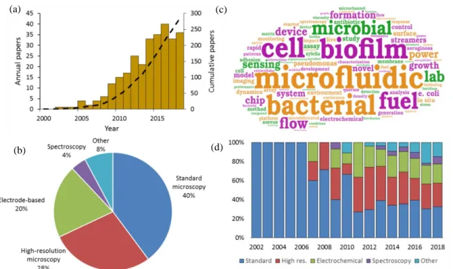
Figure 3.1. Evaluation of the literature on microfluidic studies of biofilms. (a) Annual and cumulative contributions to microfluidic studies of bacterial biofilms (gold bars and black dashed line, respectively). Contributions do not include paper, digital or static microfabricated environments. The year 2018 is adjusted to estimate total papers expected by the end of the calendar year. (b) Word cloud featuring the most popular keywords from all article titles. Break-down of techniques used in journal all articles since 2002 (c) and on a year-by-year basis (d)....44 Figure 3.2. (a) Conventional Calgary device. (b) Microfluidic planar flow cell with height of 600 µm. [48] Inset shows the direction of flow. (c) Multi-level device featuring complex fluidic circuitry designed to generate concentration gradients with built-in mixers, purpose-specific inlets, valves and separated growth compartments. [64] (d) Laminar flow-templating device for creating linear biofilms patterns using liquid-liquid interfaces to prevent growth in microchannel corners. (e) Encapsulated microenvironments containing yeast and hyphae forms of biofilm forming
Candida albicans cells after encapsulation (e1) and the more robust yeast cells when incubated in
a culture of Pseudomonas aeruginosa PA14.[69] ...46 Figure 3.3. (a) Schematic of space-time scales of different regimes associated with biofilm streamer formation. (b) An example of streamer creeping motion occurring in the time segment shown in (a) immediately before failure. [92] (c) Moving biofilm segment at intervals of 1 h. (d) Resulting biofilm viscosity (µbiofilm) after application of a semi-empirical model for [NaCl] at 0
wt% (orange), 0.05 wt% (blue), 0.1 wt% (red) and 0.2 wt% (green). ...49 Figure 3.4. (a) Captured Pseudomonas aeruginosa bacteria (red) by pre-formed streamers in serpentine channels from a biofilm of the same type from previous inoculation and growth (green). [68] (b) Dual-species 7-day-old biofilms of Pseudomonas aeruginosa (green) and Flavobacterium
sp. (red) under a range of local flow rates showing the representative biofilm morphology at each
of the nine regions in a microfluidic flow velocity gradient system. [105] (c) Confocal reflection microscopy images of S. mutans NBRC13955 biofilm growth in a microfluidic device at different growth times. [107] ...51 Figure 3.5. (a) Two-electrode electrochemical microflow cells including (a) a membraneless microfluidic microbial fuel cell, with external resistor, Rext, connecting the anode and cathode
[117] and (b) a membrane-based microfluidic microbial fuel cell. (c) Polarization curve (blue) and power output curve (red) for a microfluidic MFC. [119] (d) Power density curves for a microfluidic
xii
MFC at different flow rates. [122] (e) Current density versus time growth curves of six different electroactive biofilms during a parallel growth experiment. [126] (f) Two-electrode bioelectrochemical device with special injection valve used to record the effect of different chemical compounds on the output current from an anode-adhered Geobacter biofilm. (g) Perturbations to current output from device shown in (f) during 2 min applications of sodium fumarate. [50] ...53 Figure 3.6. (a) Schematic of a three-electrode microfluidic device with side-by-side configuration and (b) response from a working electrode-adhered Geobacter sulfurreducens biofilm in different chemical conditions, showing recovery from different concentration of toxic material. (c) Cyclic voltammetry results for the same Geobacter biofilm. (d) First derivative results from (c) showing the redox potential for the Geobacter cytochrome c groups over 9 days. [73] (e) Schematic of a three-electrode microfluidic device with sequential electrode arrangement and the upstream placement of a Au pseudo reference electrode. Blue arrow indicates direction of flow. (f) Results from an electrochemical study of de-acidification of Geobacter sulfurreducens under flow of a standard acetate nutrient solution under turnover (red) and nutrient limited concentrations (black). Inset shows the shifting CV curves that were used to monitor flow-dependant changes to biofilm pH. [131a] (g) Nyquist plots obtained from EIS in the first 65 hours of growth using similar flow cell shown in (e). Changes to biofilm resistance (h) with total flow rate (QTot) modulation before
(red bands) and after (blue dash lines) shear removal of biofilm upper layers. [100] ...56 Figure 3.7. Raman spectroscopy in microchannels. (a) Representative two-dimensional principle component analysis of P. aeruginosa biofilms for identification of clustering at different developmental stages. [148] (b) Spectra of 500 mM sodium citrate solution (red) and water (black) as measured using confocal Raman spectroscopy. Solid lines showing spectra acquired in channels with surfaces coated by an opaque silver layer, thereby eliminating the background signal from the PDMS wall, and with broken lines showing comparison with spectra acquired in the non-silver coated channel. [149] (c) Schematic of the setup for measuring low-concentration bacterial metabolites in a SERS channel down-stream of a growing Pseudomonas aeruginosa biofilm. [150] ...60 Figure 3.8. FTIR studies of biofilms in microchannels. (a) Schematic of synchrotron FTIR applied to Escherichia coli biofilms adhered to a reflective surface in an open microchannel and (b)
xiii
resulting chemical maps generated from absorption bands at 1080 cm-1 (C-O-C and C-O-P
vibrations in polysaccharides and PO2- vibrations in nucleic acids), 1130 cm-1 (C-O vibrations in
carbohydrate glycocalyx), 1240 cm-1 (vibrations from PO2- in DNA/RNA), and 1310 cm-1 (amide
III peak in proteins).[160] (c) Dual imaging of growing Pseudomonas sp. biofilm growth on top of an embedded germanium multibounce ATR element in a microfluidic device consisting of linear chemical maps from absorption band at 1540 cm-1 (amide II signal from proteins) and dark-field optical microscopy after 5 h (i), 30 h (ii) and 60 h (iii). (d) Space-time image showing the variation of amide II absorbance along the channel length (horisontal) at different times (vertical). ...61 Figure 4.1. Overall setup ...87
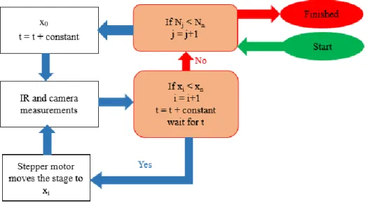
Figure 4.2. Figure 4.2. (a) Photograph of the complete system located inside of the FTIR sample compartment. Imaging system is highlighted with exploded view of optical imaging system showing (i) CMOS camera, (ii) optical lens tube held with a (iii) rack and pinion connector ring, (iv) a variable zoom knob and (v) ring light system with coupling to a fiber optic wave guide. (b) Close up microfluidic device on top of Ge ATR crystal. (c) Close up showing the stepper motor and control electronics with belt-drive coupled to the micrometer via a cog wheel. Inset shows coupling between belt and drive pulley assembly more clearly. ...87 Figure 4.3. The algorithm that is used for controlling IR instrument, camera and stepper motor. In this figure (x0, xi, xn are initial, current, and final positions on top of crystal respectively. N is the
number of measurement in each location. ...89 Figure 4.4. ATR positioning error for o-ring belt drive (orange), o-ring belt drive with computer compensation (blue) and corrugated rubber belt-drive/cog wheel (green) after cycling through ATR positions (n=60) ...90 Figure 4.5. a) Kinetic measurement: the medium flow direction is perpendicular with beam direction, tn is the time that flow reaches to xn position and V is flow rate. b) Multiplex
measurement: the medium flow direction is parallel with beam direction ...91 Figure 4.6. a) optical imaging lens, b) three-dimension rack and pinion stage, c) Optical camera, d) Fiber-lite light source, and e) Fibre Optic Ring Light Guide ...92 Figure 4.7. Pure AB medium and pure PDMS spectra are subtracted from spectra of biofilm inside microchannel to create biofilm processed spectra ...95
xiv
Figure 4.8. Different external aperture used to reduce beam width ...95
Figure 4.9. Plot of modulation vs microchannel width for three aperture sizes (0.7, 1, 1.75 mm) ...96 Figure 4.10. Hypothesized columniation from using a lens-based approach. ...97
Figure 4.11. Improving spatial resolution by adjusting center of crystal to focal point of IR beam
...97 Figure 4.12. Improving spatial resolution by reduction of IR beam width using small aperture.. 98
Figure 4.13. Interferogram intensity map across three different germanium ATR crystals: ATR1
(grey), ATR2 (orange), ATR3 (blue). ATR3 was used for the remainder of the paper. Typical scan
range of 10.7 mm is highlighted (*) ...99 Figure 4.14. Resolution measurement for different aperture size (1.5, 2.5, 3.25, 3.6, 3.9 and 4.8 mm) ...99 Figure 4.15. a) Spectra acquired from pure D2O (red), H2O (blue), and PDMS (grey). All spectra
were acquired with 64 scans using a background from pure air. b) Normalized absorbance values of characteristic peaks for H2O (νOH=3371 cm-1), D2O (νOD=2491 cm-1) and PDMS (δCH3=1260
cm-1) at different x-positions across the ATR crystal show oscillating concentrations of each.. 100
Figure 4.16. Block diagram of python code for histogram calculation ...102
Figure 4.17. Window moves on image histogram to find the correct gain. ...102
Figure 4.18. Acquired image around beginning of experiment (12 hours) using (gain = 0 and 52) is shown in which the gain is automatically created using written script. Also histogram is created for the two images to show the improvement ...104 Figure 4.19. Acquired image around middle of experiment (36 hours) using (gain = 0 and 35) is shown in which the gain is automatically created using written script. Histogram shows improvement in using bit-depth resolution ...105
xv
Figure 4.20. c) Acquired image around middle of experiment (54 hours) using (gain = 0 and 19) is shown in which the gain is automatically created using written script. Histogram shows improvement in using bit-depth ...106 Figure 5.1. (a) CAD schematic of the portable scanning ATR accessory with components identified by color. The base plate support (grey) and movable stage (blue) are controlled by micrometer positioners (grey) coupled to a stepper motor (dark green) via a timing belt (black). An optical holder (brown) immobilizes the moving stage and a multi-bounce ATR accessory with light guides (green) and ATR crystal holder (red) against the movable stage. The yellow arrow indicates the scan direction. (b) Data showing the increase in absorbance asymmetric stretch of CH3, 2960 cm-1 in PDMS during scanning from the ATR-air interface toward the ATR-PDMS
interface at the microchannel wall using different internal apertures ranging in diameter from 2.5 to 0.75 mm. Transition from microchannel to PDMS wall showing trends toward smaller rise distances as the internal aperture size is decreased (grey arrows). Black points display the highest resolution achievable (Rx = 215 µm). (c) Cartoon of a six-channel PDMS microfluidic device
(blue) with embedded ATR crystal (dark grey). IR light (red) is reduced with an aperture (grey) before hitting the beveled edge (angle of incidence 90) and then traveling through the Ge ATR crystal at a 45 degrees relative to the sensing surface. The yellow arrow indicates the same scan direction shown in (a). Inset shows a zoomed view on one channel with a breakaway view within displaying the IR beam path. The yellow arrow indicates the relative displacement of the IR probe light toward the channel wall during scanning. ...122 Figure 5.2. (a) Stitched image showing a portion of a parallel six-channel device with five enumerated separation walls. Scale bar is 1 mm. (b) Normalized IR absorbance of PDMS using IR (grey) and optical image analyses (yellow) at the indicated x-position (x-scale is applicable to (a) as well). Red lines connecting the image to 1D intensity plot are placed at the (i) channel center, (ii) straddling the PDMS channel interface and (iii) between channels. Rx is shown for the channel
to wall 2 transition. ...123 Figure 5.3. (a) The six-channel device on top of the Ge ATR crystal used for parallel assays in this work. Connections between the inlet and outlet tubing were made with metal elbow joints. Channels are filled with alternating colored liquids for visualization. Scale bar is 2 cm. Inset (top) shows the cross-section of one channel attached to a glass surface with length = 20 mm, height =
xvi
110 µm and width = 1.5 mm. The x-y axes define the coordinate system used in this paper. (b) Spectra acquired from (i) channel containing D2O (red), (ii) channel containing H2O (blue) and
(iii) PDMS spacer between two channels (grey). All spectra were acquired with 64 scans using a background from pure air. (c) Normalized absorbance values of characteristic peaks for H2O (3370
cm-1), D2O (2490 cm-1) and PDMS (1260 cm-1) at different x-positions across the ATR crystal.
...124 Figure 5.4. (a) IR spectra of a Pseudomonas sp. biofilm (60 h) collected from a single channel. The highlighted peaks result from CH2 (2920, 2850, and 1450 cm-1), amide I (1640 cm-1) amide II
(1545 cm-1), amino acids (1400 cm-1), and phosphate-containing groups (1085 and 1235 cm-1). (b) Growth of the amide I and II bands in the range of 1300–1800 cm-1 at 20 (blue), 25 (red), 35 (green) and 50 h (purple). (c) Optical micrographs of a portion of the same channel measured in (b) at the same growth times. Scale bar is 500 µm. (d) Average absorbance values (red) and average optical intensity (black) versus time. Flow rate Q = 0.2 mL·h-1. All spectra are the results of spectral subtraction of pure PDMS and water. ...126 Figure 5.5. (a) Average intensity of amide II absorption band (blue) and pixel intensity (orange) for 6 sequential Pseudomonas sp. biofilm cultures from (i) separate experiments conducted on different days with different inoculum and (ii) experiments conducted in parallel on a six-channel device with the same inoculum. Error bars represent the standard deviation (STD). In all cases, an AB nutrient medium with 10 mM acetate was applied with a flow rate Q = 0.2 mL·h-1 in channels
with the same dimensions (w = 1.5 mm, L = 2 cm, h = 100 µm). (c) Repeatability enhancement (RE) for microscopy and IR spectroscopy. Inset shows RE during the first 5 hours. (d) Growth experiments with varying concentrations of ethanol added to an AB nutrient solution immediately following inoculation with concentrations (w/w%) of 0 (light blue), 1 (orange), 2 (grey), 3 (yellow), 4 (dark blue) and 5 (green). (e) Growth experiments with ethanol concentrations (w/w%) of 0 (light blue), 3 (orange), 5 (grey), 10 (dark blue), 20 (yellow) and 70 (green) added to an AB nutrient solution 14 h following channels inoculation. ...129 Figure 5.6. (a) Schematic showing a segment of an ATR crystal (blue) containing the microchannel (black) relative to the IR beam path (red) at different scan positions. (b) Image pairs consisting of a linear map of the amide II absorbance and a stitched optical micrograph at (i) 5 h, (ii) 30 h, and (iii) 60 h, as indicated in (c). Scale bars are 1.5 mm. (c). Space-time image showing
xvii
the variation of amide II absorbance along the channel length (horizontal) at different times (vertical). Arrow indicates the scan direction along the x-axis and the direction of time along the vertical axis. Colored arrows indicates x-positions at 0.8 mm (blue), 5.5 mm (orange), and 9 mm (grey) of plots in (d). (d) Time-dependent amide II absorbance at the x-positions marked by colored arrows in (c). The black dotted line is the average amide II absorbance at all positions throughout the channel. The time axis in (d) is matched to that in (c), and the color bar intensities are matched to the absorbance on the horizontal axis. The color bar defines the absorbance values for (b), (c)
and (d). ...130
Figure 5.S1. (a) Photograph of the complete system located inside of the FTIR sample compartment. Imaging system is highlighted with exploded view of optical imaging system showing (i) CMOS camera, (ii) optical lens tube held with a (iii) rack and pinion connector ring, (iv) a variable zoom knob and (v) ring light system with coupling to a fiber optic wave guide. (b) Close up microfluidic device on top of Ge ATR crystal. (c) Close up showing the stepper motor and control electronics with belt-drive coupled to the micrometer via a cog wheel. Inset shows coupling between belt and drive pulley assembly more clearly. (d) a diagram showing the angle of incidence against the ATR beveled edge and the optical beam path within. ...139
Figure 5.S2. (a) Aperture diameter and signal at the MCT detector and (b) IR beam divergence as a function of aperture setting. Values are nominal values as reported by the spectrometer manufacturer. ...140
Figure 5.S3. Flow chart of the custom control program. ...143
Figure 5.S4. Program front panel for “Camera initialization”. ...144
Figure 5.S5. Program front panel for “Motor stage initialization”. ...145
Figure 5.S6. Program front panel for “Measurement process”. ...146
Figure 5.S7. Program front panel associated with the gain control adjustment. “High-Low” button toggles between regular 8-bit image and the same image with colors showing empty pixels (blue representing pixels with bit values = 0) and saturated pixels (red, representing pixels with bit value=255). Real-time results in the displayed image are in regular or High-Low modes during
xviii
manipulations of gain or exposure parameters. The algorithm developed for automated gain control (see Figure 5.S6 could also be used but was not implemented. ...147 Figure 5.S8. Block diagram of automatic gain assignment of camera in optical camera, where Imax is the average value of the 5% most intense pixels in the image and Iceiling is the
maximum bit value that the camera can register. ...148 Figure 5.S9. Interferogram intensity map across three different germanium ATR crystals: ATR1 (grey), ATR2 (orange), ATR3 (blue). ATR3 was used for the remainder of the paper. Typical scan range of 11 mm is highlighted (*)...149 Figure 5.S10. Channels filled with water and D2O alternatively, related monitored peaks for H2O
(blue), D2O (red), and PDMS (grey) are 3371, 2491, 1260 cm-1 for (a) 4 channels (b) 5 channels.
...149 Figure 6.1. (a) A schematic of the 6 channel device oriented to the underlying ATR crystal with its channels co-linear with the IR beam direction (right to left). Channel dimensions are not to scale. Blue channels correspond to channels sealed with non-plasma treated ATR portions. An image of the multibounce Ge ATR crystal with two 0.2 mL water droplets applied to its surface following plasma treatment to one side, with the other being protected plastic film. Dashed line shows the interface between the protected and exposed sides. Scale bar represents 1 cm. (b) FTIR spectrum from the germanium ATR surface in air following 90 s exposure to air plasma. A background spectrum was acquired from the same ATR crystal before plasma treatment ...157 Figure 6.2. Time-varying absorbance bands in different spectral windows showing changes to (a) CHx, (b) C=O/COO- and (c) GeOx after exposure to air plasma gas. The grey curve in (c) shows
the spectrum in air after surface exposure to plasma, with a background of the crystal in air before plasma exposure. In all cases, a spectrum acquired at t=0 was used as a background ...158 Figure 6.3. Surface recovery plots for plasma treated ATR crystals under (a) nutrient flow conditions and (b) during biofilm growth conditions. Absorption peaks followed were GeOx
(black), CH2 (red) and C=O/COO- (blue). ...158
Figure 6.4. Time-varying spectral bands during biofilm growth in plasma (a) and non-plasma (b) treated channels. Highlighted bands are for amide I (i), citrate (ii) and amide II (iii).. ...160
xix
Figure 6.5. Normalized plots of (a) ATR-FTIR measurements of amide II absorbance values versus time and (b) optical intensity versus time of plasma treated channels (red and orange) and non-plasma treated channels (grey). Dashed and solid lines show growth trends during lag phase and rapid growth phase, respectively. Inset images show examples of biofilm formation against plasma treated (upper) and untreated (lower) ATR surfaces at 40 h ...161 Figure 6.S1. Surface recovery spectra in time for plasma treated ATR crystals under sterile nutrient flow conditions. Focus on CH2,3 peaks (a), C=O/COO- contaminants and citrate (b) and
GeOx peaks (c). Dashed line in (c) shows absorbance band from GeOx groups at the ATR crystal
surface in air, immediately after plasma treatment (using a single beam spectrum after cleaning, but before plasma exposure as a background). For all time-varying spectra, a single beam measurement was acquired immediately after inoculation (t = 0) was used as a background for the subsequent experiments ...167 Figure 6.S2. Recovery of CH2 (red), C=O/COO- (blue), and GeOx (black) as measured at 2950,
1715, 735 cm-1, respectively, for sterile growth medium conditions. Recovery is the reduction in height of each negative peak, normalized by the peak size at t=0 ...167 Figure 6.S3. (a) schematic showing a cross-section of the PDMS device (grey) against an ATR element (orange) under clamping contact (arrows). Increased clamping pressure can cause the PDMS material to deform and buckle resulting in contact with the ATR crystal. (b) Absorbance bands from PDMS as clamping pressure is increased. ...168 Figure 6.S4. A 6-channel PDMS device attached to the ATR crystal by plasma only (a) and by clamping (b). Colour dye was added to channels for visualization. ...169 Figure 7.1. Cartoon schematic showing the linear scanning ATR-FTIR technique applied to a single microchannel for one-dimensional mapping along the x-direction. The setup includes a Ge ATR crystal (grey) contacted by a PDMS microfluidic device and a top-side reflection microscope consisting of a digital camera (dark grey) with focus objectives (light grey) and integrated illumination (yellow). Arrows show the IR light path through the crystal for previous imaging positions (pink) and the current scan position (red). The axes define the x-, y- and z-directions referred to in this work. ...180 Figure 7.2. Microscope images of P. fluorescens biofilm growth within the middle 16 mm of a channel with overall length of 22 mm at t = 24 h (a), 25.5 h (b), 27.5 h (c) and 60 h (d). In all
xx
images, a red dotted outline shows the position of the bubble at t = 22 h. Yellow dotted lines in (a) and (b) highlight the contracted bubble size at the time of imaging. In (d), the axes define the x- and y-directions, the scale bar is 500 µm, and coloured rectangles show the positions where further optical analyses were acquired corresponding to the channel positions (e) x = 1 mm (blue), x = 5.5 mm (red) and x = 16 mm (green). The flow direction is from left to right. (e) Average pixel intensity versus time for rectangular regions of interest (0.6 x 1.1 mm) centred at x = 1.0 mm (blue), x = 5.5 mm (red) and x = 16 mm (green). The blue, red and green colours match the box colours in (d). Error bands were obtained from the standard deviation of the measurement. Lagnobubble and Lagbubble correspond to the lag phase for biofilms away from and within the original bubble position ...179 Figure 7.3. Stacked spectra from time-evolving P. fluorescens biofilms in positions of (a) x = 1 mm, (b) 5.5 mm and (c) 17 mm from 0 to t = 60 h. Five times more spectra were acquired than are shown to reduce figure complexity. (d), (e) and (f) present two spectra at 26 h (dotted line) and 60 h (solid line) based on the corresponding highlighted spectra from the time-series data in (a), (b) and (c). ...181 Figure 7.4. (a) Percentage of the channel occupied by an air bubble, (b) biofilm pixel intensity, (c) absorbance of protein amide II and (d) absorbance from lipid C=O vibration, each as a function of downstream position (x-axis) and time (y-axis). The lag phase as measured from microscopy (Lagoptical) and amide II absorbance (LagamideII) is compared at 6 mm (b) and (c), respectively. Colour bars quantify the measured property. Divisions in colour bars in (b)-(d) denote contour values in their corresponding figures ...185 Figure 7.5. Changes in protein absorbance (solid lines and symbols) and lipid absorbance (dashed lines, open circle). Measurements were acquired from positions x = 6 ± 1.5 mm (red), x= 1.5 ± 1.5 mm (blue) and x = 14.5 ± 1.5 mm (green). The black dashed line reports the time-varying percentage of the channel occupied by the bubble ...186 Figure 7.6. Vibrational frequency space-time map for amide II bands in proteins (a). Overlapped time-varying spectra at x = 14 mm channel position (b). Arrows show the position of the amide II band at t = 0 (blue) and t = 60 h (red) ...187
xxi
List of Tables
Table 1.1. Some typical analytical methods have been used for studying biofilms ...7
Table 1.2. Electromagnetic spectrum ...19
Table 1.3. Properties of typical ATR crystal materials ...22
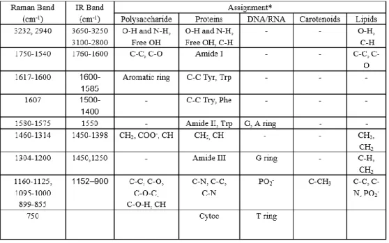
Table 3.1. Band assignments for Raman and IR spectra of typical bacterial biofilms ...57
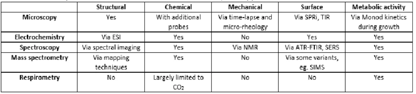
Table 3.2. A comparison of different tools to different analytical applications ...65
Table 4.1. Full property of imaging lens is shown in details ...92
Table 4.2. Full specification of the camera. ...93
xxii
List of Equations
Equation 1.1. Navier-Stokes equation ...8 Equation 1.2. Navier-Stokes linear equation ...8 Equation 1.3. Reynolds number ...8 Equation 1.4. Hydrodynamic resistance ...9 Equation 1.5. Electrical resistance ...9 Equation 1.6. Bohr frequency condition ...17 Equation 1.7. Relationship between frequency and wavelength ...17 Equation 1.8. Wavelength and wavenumber relation ...17 Equation 1.9. Hooke’s law ...19 Equation 1.10. Penetration depth is wavelength dependent ...22 Equation 1.11. Beer-Lambert law ...23 Equation 4.1. Modulation ...96 Equation 5.1. Repeatability enhancement (RE) ...127
xxiii
List of abbreviations
A Absorbance
AB Agrobacterium growth media AFM Atomic Force Microscopy ATR Attenuated total reflection c Concentration
CLSM Confocal Laser Scanning Microscopy dp Depth of penetration
E Energy
EPM Extracellular polymeric matrix FTIR Fourier-transform infrared IR Infrared
h Plank’s constant I Electric current k Bond force constant L Characteristic length
LB Lysogeny broth growth media n Refractive index
P Pressure
PDMS Polydimethylsiloxne Q Volumetric flow rate R Electrical resistance
xxiv
r Reduced mass Re Reynolds number
RH Hydrodynamic resistance
SERS Surface Enhanced Raman Spectroscopy u Velocity V Voltage θ Incident angle ε Absorbance coffiecient µ kinematic viscosity ∇ Laplacian 𝜌 Mass density 𝜈̅ Wavenumber λ Wavelength 𝜈 Frequency
xxv
Acknowledgments
Foremost, I would like to express my sincere gratitude to my supervisor Prof. Jesse Greener for his constant support, motivation, patience and knowledge. His valued guidance helped me in my research and writing of this thesis.
I would like to thank François Paquet-Mercier, who as a good friend was always willing to help and give his best suggestions. Also a huge thank you to all my amazing friends and colleagues (Mehran Abbaszadeh Amirdehi, Mirpouyan Zarabadi, Farnaz Asayesh, Erica Rosella, Nan Jia, Md Ramim Tanver Rahman, Lingling Gong, Tianyang Deng, Brandon Lemelin-Donnelly and Kimberly Côté-Vertefeuille), for their help in this project and for their friendship and support that will make my PhD period a beautiful memory. A special thanks to my family. Words cannot express how grateful I am to my parents for supporting me in achieving this.
xxvi
Foreword
The following section lists the published work for each chapter including the contribution of each author.
Chapter 4.
M. Pousti, M.P. Zarabadi, M.A. Amirdehi, F. Paquet-Mercier, J. Greener, Microfluidic bioanalytical flow cells for biofilm studies: a review, Analyst, 144 (2019) 68-86.
Contribution: In this review paper M.P.Z. and M.A.A. contributed on electrochemical measurements section, F.P.M. focused on optical imaging section. M.P. focused on Spectroscopy and chemical imaging sections and also collecting and organizing all references. The manuscript writing and editing was mostly done by J.G. and M.P.
Chapter 5.
M. Pousti, M. Joly, P. Roberge, M.A. Amirdehi, A. Bégin-Drolet, J. Greener, Linear scanning ATR-FTIR for chemical mapping and high-throughput studies of Pseudomonas sp. biofilms in microfluidic channels, Analytical Chemistry, 90 (2018) 14475-14483.
Contribution: M.P. and J.G. formed the concepts of project and planned the experiments. M.P. fabricated flow channels, bacterial preparations, and conducted all experiments and analysis. ATR system development and programming was initially done by M.P.. M.J. and P.R. created a user-friendly interface. The manuscript writing and editing was mostly done by J.G. and M.P.
Chapter 6.
M. Pousti, J. Greener, Altered biofilm formation at plasma bonded surfaces in microchannels studied by attenuated total reflection infrared spectroscopy, Surface Science, 676 (2018) 56-60. Contribution: M.P. and J.G. formed the concepts of project and planned the experiments. M.P. fabricated flow channels, bacterial preparations, and conducted all experiments and analysis. The manuscript writing and editing was mostly done by J.G. and M.P.
1
Introduction
Biofilms are widespread in most ecosystems. They can be formed by most microorganisms. Microbial biofilms are multicellular communities of bacteria, adhering to a surface, surrounded by varying amounts of a self-produced extracellular polymeric matrix (EPM). Research into biofilms is accelerating due to their roles in the environment, human health, industrial biofouling and their potential as biocatalysts. Among the main factors contributing to biofilm development and its mature properties are the applied hydrodynamic conditions and nutrient concentrations. Growth of surface-adhered bacterial biofilms is a major area of interest in medical, biotechnical and environmental research. Microfluidic present high surface area environments with strong control over liquid conditions for real-time studies of biofilm growth and contamination. Combined with modern in situ analytical characterization, microfluidic studies of biofilms are poised for strong growth in research and development. Microfluidics is becoming increasingly popular among the biofilm research community because of its ability to better control relevant parameters for biofilms. The study of biofilms using microfluidics is a rapidly advancing area, occupying scientists and engineers from all backgrounds. As part of this work we have exhaustively reviewed the literature.
Infrared (IR) spectroscopy is an excellent method for “on-chip” biological studies because it can make label-free measurements of chemical properties in flow without tracers or dyes. Even though it can be a strong technique for studying biofilms, there are very few literature examples using IR spectroscopy combined with microfluidics due to challenges of integration.
This PhD thesis focuses on developing a fully automated linear scanning attenuated total reflection (ATR) accessory for Fourier transform infrared (FTIR) spectroscopy. The approach is based on the accurate displacement of a multi-bounce ATR crystal relative to a stationary infrared beam. To ensure accurate positioning and to provide a second sample characterization mode, a custom-built microscope was integrated into the system and the computerized workflow. Custom software includes automated control and measurement routines with a straightforward user interface for selecting parameters and monitoring experimental progress. This cost-effective modular system can be implemented on any research-grade spectrometer with a standardized sample compartment. The system was validated and optimized for use with microfluidic ATR flow cells containing
2
growing of Pseudomonas sp. bacterial biofilms in three published studies. The complementarity among the scan positioning accuracy, spatial resolution of the measurement and the microchannel dimensions paves the way for parallel biological assays with real-time control over environmental parameters with minimal manual labor. By rotating the channel orientation relative to the beam path, the system could also be used for acquisition of linear biochemical maps and stitched microscope images along the channel length.
3
1. Chapter 1: Literature review
1.1. Bacteria and their Biofilms
Bacteria generally exist in two states. In the planktonic state bacteria can swim through the liquid phase using appendages called flagella. In the sessile form, bacteria adhere to surfaces using chemical-physical attachment mechanisms. Bacteria in the planktonic state have been the focus of numerous biological studies, but in fact this is not their typical state in nature. Following about 4 decades of intensive studies, it is known that bacteria in fact are mostly found in sessile communities encased in a self-produced extracellular polymeric matrix (EPM). These formations are called biofilms. Polysaccharides, DNA, and proteins are the three major components of EPM that work as a glue to keep cells attached to surfaces and together. [1] Biofilms are interesting materials to study because of their complex, stimulus-responsive-structures with special morphologies, mechanical and chemical properties, which are spatially heterogeneous and change in time. Biofilms are also important systems of study in medical sciences and in industry. For example, in medicine biofilms are distinguished as an important source of resilient pathogenic bacteria that can cause disease, chronic infections and tooth decay. [2] In industry, problems of biofouling and clogging problems in flow systems and increase tolerance to antibacterial agents (problems to avoid) and wastewater treatment.[3, 4] Biofilms are especially interesting to chemists and materials scientists as potential functional, catalytic materials with applications in electricity production, environmental bioremediation, chemical synthesis etc. [5] To advance this area of research it is important to accurately characterize mechanisms involved in the biofilm growth, and functionality. [6]
The biofilm development process is typically expressed in 5 stages: (1) transport and initial attachment of microbes, (2) irreversible adhesion or attachment, (3) microcolony formation, (4) maturation of the biofilm and (5) detachment and dispersion of the cells. In fact, this is a simplistic model, which ignores the fact that planktonic bacteria are constantly being ejected from the biofilm at all stages, as discovered recently using a microfluidic setup. [7]
4
In general, the initial step of biofilm formation is the adhesion of the bacteria to surfaces by unspecific physicochemical interactions. These interactions are guided by the particular charges and hydrophobicities of both bacteria and the materials involved. [8] Bacteria and most natural and artificial surfaces investigated so far are negatively charged. [9-12] Therefore, adhesion will take place only when the resulting electrostatic repulsion is overcome by attractive forces like, e.g., van der Waals forces or hydrophobic interactions between bacterial surface polymers and the solid surface. [8, 13] Bacteria are also very efficient at modifying potential attachment surfaces by producing a molecular conditioning layer which can enhance initial attachment process. [14] For example, bacteria often attach themselves to glycoproteins present in the conditioning layer. The conditioning layer can also consist of different biomolecules such as proteins and polysaccharides and helps to keep the bacteria attached to the surface. After bacteria become irreversibly attached, they begin to rapidly reproduce by cell division forming microcolonies. After the surface is covered in a layer of bacteria the biofilm begins to thicken creating three-dimensional structures. Many bacteria generate complex mushroom-like architectural features. These structures are characterized by a somewhat spherical cap, or canopy, atop a narrower base, often referred to as the stalk. Researchers distinguish between the cells that continue to explore the surface and those that form microcolonies as two distinct subpopulations. The motile (cap-forming) subpopulation
(1) (2) (3) (4) (5)
Figure 1.1. Depiction of typical stages of biofilm formation. (1) Transport and initial attachment of microbes to a molecular conditioning layer, (2) irreversible adhesion or attachment mediated by small amounts of EPM (blue), (3) formation of microcolonies and continued accumulation of EPM, (4) thickening and structuration of the biofilm and (5) detachment and dispersion of the cells individually (red dashed) or in clumps known as flocs (purple dashed).
5
migrates to the top of the microcolonies formed by the non-motile (stalk-forming) subpopulation, generating a mushroom-like structure. [15] This process has been observed recently in two microfluidic publications. In one, initial formation of EPM was co-localised with stalk portion of the biofilm as revealed by fluorescence staining techniques and perturbations applied by slow-moving bubbles, respectively. [16] In a second paper, a microfluidic electrochemical cell with in line ATR-FTIR spectroscopy detected the reduction in biomass associated with the formation of voids at the attachment surface. Parallel measurements by confocal laser scanning microscopy (CLSM) visualized the same process. [17] Mature biofilms undergo a process of detachment that initiates in the center of caps. [18] This results in the creation of a fluid-filled cavity (stage 4) inside the cap in which planktonic cells are visible. [19] The cavity becomes larger over time, eventually breaking open, allowing the planktonic cells to escape and presumably form biofilms elsewhere [19, 20]. It is important to note that the dispersion of the biofilm can also occur during each stage of its growth [21]. Recently, a microfluidic method was developed to continuously study the changes in biofilm mechanical properties during growth. [22, 23] The viscosity measured as a function of time revealed a rapid thickening process near the end of the rapid growth phase. During this process, the viscosity was measured to increase by more than an order of magnitude in less than 10 hours. The time at which this process occurred and the maximum viscosity after the thickening process was found to be very sensitive to ionic strength. [22] A method of image subtraction revealed a new method of streamer formation by “sudden partial detachment”, which occurred immediately after the rapid thickening process finished. [24] Detachment seems to be common among all biofilms, which can also be responsible for bacterial cell proliferation individually or in clumps (flocs).
1.1.1. Biofilm chemical components and importance of early detection
Bacteria living in biofilms have many advantages over planktonic life. The EPM exhibits a high degree of resistance to antimicrobial agents and other harsh conditions. Unprotected bacteria in steps 1 and 5 (Figure 1.1) are relatively easy to kill with antibiotics or other chemical treatments because they do not benefit from EPM protection. However, sessile bacteria surrounded by EPM in biofilms are more resilient. Therefore, early detection of EPM molecules can be a very important method to detect transitions to biofilms before they become well-established. This amounts to an
6
interesting challenge for analytical chemists due to the time-changing and species-dependent nature of the EPM molecules.
1.1.2. Biofilm measurement
Analytical chemistry methods are promising methods for studying a range of biofilm properties, such as chemistry, structure and mechanical properties. Table 1.1 shows popular analytical methods that have been used for studying biofilms. New approaches using spectral imaging hold promise for deeper investigations and are reviewed elsewhere. [25] In the Table weaknesses and advantages for each approach is listed. Among them, microfluidics stands out as an excellent method for controlling environmental conditions, which is a prerequisite for accurate measurements by any measurement modality. It is also promising for high-throughput screening via continuous manipulation of flow conditions or in highly parallelized microchannels. Thus microfluidic devices are expected to contribute to the study of biofilms, especially when combined with existing powerful instrumental analysis, such as advanced imaging, electrochemical tools and spectroscopy. [6] This combination of microfluidic devices with analytical methods is a great challenge and is one of the primary goal of this project. Finally, the ability to implement multiple laboratory experiments in one device and to collect data for accurate statistical analysis makes microfluidics desirable for exploring various aspects of microbial biofilms. [26]
1.2. Microfluidics
Microfluidics is described as the science and technology of manipulating fluid flow at the microscale. This includes all aspects of device design and fabrication, as well as their use for processing and controlling liquid flow inside purpose-specific micrometer-scale channels. Many biological and chemical studies benefit from microfluidics due to its superb control over reaction parameters, ability for parallel and high–throughput assays, inexpensive fabrication, small liquid volume, control over temperature, ability to manipulate concentrations in space and time, ability to geometrically confine cells, rapid and precise analysis and the ability to integrate several laboratory functions on a miniaturized chip. [6, 28]
In the following sections relevant characteristics of fluid flow and molecular transport mechanisms within microfluidic systems are explained.
7
Table 1.1. Some typical analytical methods have been used for studying biofilms. [27]
Technique Usage Benefits Limitations
Regular microscopy 1) Lab studies with or without stains 1) Sensitive
2) High resolution (≈ 0.3μm ) 1) Low throughput 2) Semi-quantitative 3) Flat, optically transparent Confocal microscopy 1) Lab studies with stains and labels
2) 3D profile (confocal laser scanning microscopy)
3) Diffusion studies
1) Sensitive
2) High resolution (≈ 0.3μm ) 3) Works well with flow cells
1) Low throughput 2) Semi-quantitative 3) Flat, optically transparent 4) Requires a fluorescent sample
Scanning electron microscopy (SEM)
1) Visualize biofilms on clinical samples 2) Confirm microscopy on in-vitro test
1) Able to see all bioburden regardless of stain affinity
2) High x-y resolution (≈1 nm)
1) Low throughput 2) Not real-time 3) May require additional sample preparation 4) Qualitative Atomic force
microscopy (AFM)
1) Explore thickness and morphology of biofilm
2) Test adhesion force
1) High z-resolution (0.1-1 nm) 2) Potential to obtain information on forces
1) Low throughput 2) No composition information
3) Requires open system Genetic assays 1) Clinical Diagnostics
2) Epidemiology
3) Species determination on wounds and explanted devices
1) Potential to give species information 2) More rapid than culture methods
1) Quantitative sampling difficult
2) No biofilm mass or EPM information
3) Extensive sample Microplate assays Laboratory screening of biofilm growth 1) Potentially higher throughput
2) Potentially quantitative
Slower if culturing needed Mass spectroscopy 1) Proteomics of biofilm species
2) Metabolic analysis 3) Signaling molecules 1) 100s to 1000s of compounds identified 2) High throughput 1) Sample preparation cumbersome 2) Requires lengthy separation Imaging mass spectroscopy
1) Biofilm chemical composition distribution
2) Living biofilm analysis
1) In situ analysis of intact biofilm 2) Lateral and depth variations can be explored
1) Semi-quantitative 2) Matrix interference 3) Ion suppression effects Raman 1) Chemical analysis of biofilms
2) Can be extended to imaging in 2- and 3 dimensions
1) Stains or labels are not required 2) Multiple analytes
3) No interference from water
1) Low sensitivity, which can be enhanced with plasmonic materials 2) Long analysis times IR 1) Quantitative and qualitative chemical
analysis of biofilms 2) Living biofilm analysis
1) In-situ analysis of intact biofilm 2) Stains or labels are not required 3) Multiple analytes
4) Almost no sample preparation needed
1) Low sensitivity 2) Difficult to extend to spectral imaging
3) Water is highly absorbing Microfluidics 1) High throughput drug screening
2) Metabolic profiling
1) Small sample requirements (<1 μl) 2) Long duration experiments 3) Less biohazardous waste 4) Low potential for contamination
1) Few commercial formats 2) Difficult to test materials (Catheter tubing, cement, etc.)
Fabrication of microfluidic devices differs from macroscale ones. One generally cannot scale a macro device down and then expect it to work in microfluidics applications. When the dimensions of a device becomes smaller, the physics or behavior of the system under study will change. Thus some forces that govern macroscopic world might not be dominant here, like appearance of capillary forces in a small flow system. What follows is a short mathematical and semi-empirical description of some of the changing physical behaviors of fluids in microfluidic system. Such environments provide new opportunities to investigate a range of different like; fluid viscosity, pH, capillary electrophoresis, flow cytometry, PCR amplification, DNA analysis and chemical gradient formation. [29]
8
In general, incompressible flows are governed by as the Navier-Stokes equation (Equation 1.1):
∂u
∂t + u × ∇u = − ∇p
ρ + μ∇
2u
Equation 1.1
where ∇ is Laplacian, 𝜌 is the mass density, 𝑢 (m/s) is the velocity and μ (m2/s) is the kinematic
viscosity of the liquid phase. Kinematic viscosity is the measure of the inherent resistance of a fluid to flow when gravity is the only external force applied, calculated by dividing the dynamic viscosity of fluid to its density, a force-independent quantity. In this equation there are two important terms that make the difference between microfluidic flows and large-scale flows, the term 𝑢. 𝛻𝑢 corresponding to the inertia of fluid and the term μ∇2𝑢 responsible for accounting viscosity in fluids. In micro flow (in microfluidic channels), inertia is damped by viscous effects and the term corresponding to inertia can be neglected in above Navier-Stokes equation, which leads to a linear partial differential equation (Equation 1.2) that is easier to solve and gives rise to a unique solution. [30]
∇p ρ = μ∇
2u Equation 1.2
The flow of a fluid through a microfluidic channel can also be characterized by the Reynolds number that provides an estimation of the ratio of inertial forces/viscous forces (Equation 1.3): Re =uL
μ Equation 1.3
where L is thecharacteristic length depends on geometrical shape (for example L will be the width in a rectangular microchannel).
1.2.1. Pumping mechanism
Two common means of achieving fluid transport in microfluidic systems are pressure-driven flow and volumetric-driven flow. Due to the high surface area to volume ratios in micro-channels, many interfacial phenomena drive the fluid behavior. Such phenomena include wetting properties, surface tension, capillary effects and electrokinetics.
9
1.2.1.1. Pressure-driven flow
Pressure-driven pumps provides highly stable pulseless liquid flow and is the best available pump for droplet formation and other applications requiring high accuracy manipulation of flow. Generally, the air headspace above a liquid in a sealed container can be accurately pressurized to drive liquid into connecting tubing, which is connected to the microfluidic device. The flow rate that results from the application of an upstream pressure source depends on the hydrodynamic resistance (Equation 1.4), much in the same way as current flowing through an electric circuit from the application of an applied voltage depends on the electrical resistance of the circuit (Equation 1.5). In Equation 1.4 P is pressure, Q is flow rate and RH is hydrodynamic resistance. In Equation
1.5, V is voltage, I is electric current and R is electrical resistance.
P = Q×RH Equation 1.4
V= I×R Equation 1.5
New market solutions exist for pressure-driven flow system which are specifically designed for microfluidic applications, that can accommodate wide pressure and flow rate ranges, closed-loop flow rate control, often with computer interface, automation and peripheral accessories such as automated valves, de-gassing units and other physiochemical sensors. These systems can accommodate source containers from milliliters to several liters, enabling a wide range of flow rates to be applied. It brings ultimate flexibility to scientists who can use it for small-scale, single- or multi-chip systems.
1.2.1.2. Volumetric driven flow
Volume-driven flows use mechanical method for forcing liquid into connective tubing at know flow rates. Most popular approaches include syringe pumps and peristaltic pumps. Syringe pumps are usually preferred for microfluidic applications because of their excellent control over solution disbursement at very low and precise flows rates which is less pulsing that peristaltic. These pumps usually consist of a motor that drives a screw or gear mechanism that advances either the plunger or barrel of the syringe at a predetermined rate. They also can include automated computer control, alarms, electronic communications and triggers. In most pumps the syringe containing the infuscate must be manually replaced once it has emptied to continue the infusion.
10
1.2.2. Materials for microfluidics
Microfluidic devices feature very large surface area to volume ratios, enhancing the interaction between the material of microchannel wall and the solution environment. The constrained physical dimensions of microchannels often result in the need to position optical characterization equipment outside optical microchannels. In cases where probes and other functional elements can be interfaced directly with the microreactor, the mechanical properties of the device should be robust. A review of materials for microfluidics manufacture and their suitability for functional material synthesis and characterization is presented below. Common viable compatible materials used are silicon, metal, silica, polymeric or paper.
1.2.2.1. Polymers
Polymers play a dominant role as microfluidics device fabrication materials due to their low cost, the wide range of formulations available, the ease of processing, and the potential for mass production. For these reasons, sales of polymer microfluidics devices currently account for approximately 50% of the world market. Moreover, polymer materials can be transparent, enabling optical characterization. Typical polymeric materials used for microfluidics include thermoplastics, such as polyethylene terephthalate (PET), polymethyl methacrylate (PMMA), polycarbonate (PC) and polyimide (PI). These materials benefit from good optical transparency in the visible and in some cases in the UV, wide range of machining and moulding tools with high fidelity, simplicity in the modification of surface properties, biocompatibility or bioactivity, durability, a range of chemical compatibilities and availability of medical grade (low-toxicity) formulations. Among the most commonly used materials is an elastomeric material called polydimethylsiloxane (PDMS). Its wide use, particularly in academic research and for developmental purposes, results from its low cost, easy demolding and its good self-adhesive properties following surface activation using O2 plasma or UV light exposure. Enhanced bonding
techniques for PDMS can result in stronger bonds and seals between layers, [31] but they are still more prone to debonding and channel deformation than devices made from more robust materials such as glass or metal. Other major drawbacks of PDMS include its permeability to oxygen and small molecules, limited chemical compatibility and its propensity to swell in some solvents. As a result, there has been a recent focus on developing new hard plastic-based microreactors, which could enable operation at high pressures and allow interconnectivity with other instrumentation.
11
The rise of polymer-based microfluidics platforms has paved the way for customized microfluidics and thus maximized the flexibility of these systems. Micropatterning of polymer materials can be accomplished by a number of techniques such as curing, micromachining, [32] laser ablation, [33] hot embossing, [34, 35] and injection molding. [36] Bonding the patterned layer to a planar layer for chip-based devices can be accomplished using heat, epoxies, and surface activation techniques. With a few exceptions, most polymers are hydrophobic, which can present challenges in forming oil droplets in water phase (see Section 4) due to the preference of the emulsified monomer-phase precursor liquids which wet the channel walls over the aqueous carrier phase. Surface treatment techniques can change the wetting properties of microchannel walls, making it more suitable for emulsification of a range of liquid precursors. For example, exposure to O2 or air plasma can add
OH groups to exposed surfaces, thereby converting the wall to hydrophilic. Chemically treated thermoplastics have also been demonstrated to alter the wetting properties and to enhance resistance to organic solvents, as demonstrated by a series of papers involving surface modification of polycarbonate. [37-39] Generally, surface treatments of elastomers are less effective than for rigid polymers due to the higher mobility of surface groups.
1.2.2.2. Glass
Glasses, quartz and fused silica are widely used materials for microfluidics reactors. [40] Their advantages include excellent resistance to most chemical environments (with the notable exceptions of HF and other acids), high temperatures and pressures. Glass is typically hydrophilic, making it an excellent choice for emulsifying oil in water (Section 4), and has excellent transparency in the visible region, enabling optical observation and measurements. However, glass is extremely brittle. In addition, it is costly and time-consuming to manufacture as compared to plastic materials. Acid (wet) etching through a chemically resistant mask is usually used in fabrication. Typically, hydrofluoric acid (HF) is used for rapid glass etching, but the etching solution often includes a blend of acids to solubilize all by-products. Wet etching of amorphous glass materials results in isotropic feature, which produces hemispherical channel cross-sections. A planar coverslip can be bonded to an etched glass device using high temperature, pressure, or an intervening layer of adhesive. Creating through holes in glass is relatively difficult, requiring sandblasting, laser drilling, diamond drill bits or deep wet etching, making interface of fluidic connections and other peripheral devices challenging. New methods to partially etch or cut through thin glass slides include femtosecond laser etching and spark assisted chemical engraving. Both
![Table 1.1. Some typical analytical methods have been used for studying biofilms. [27]](https://thumb-eu.123doks.com/thumbv2/123doknet/3205456.91611/33.918.110.831.135.760/table-typical-analytical-methods-used-studying-biofilms.webp)