HAL Id: tel-02274370
https://pastel.archives-ouvertes.fr/tel-02274370
Submitted on 29 Aug 2019HAL is a multi-disciplinary open access archive for the deposit and dissemination of sci-entific research documents, whether they are pub-lished or not. The documents may come from teaching and research institutions in France or abroad, or from public or private research centers.
L’archive ouverte pluridisciplinaire HAL, est destinée au dépôt et à la diffusion de documents scientifiques de niveau recherche, publiés ou non, émanant des établissements d’enseignement et de recherche français ou étrangers, des laboratoires publics ou privés.
Dynamic management of tracking ressources for
hyper-manoeuvring targets
Marion Pilte
To cite this version:
Marion Pilte. Dynamic management of tracking ressources for hyper-manoeuvring targets. Automatic. Université Paris sciences et lettres, 2018. English. �NNT : 2018PSLEM068�. �tel-02274370�
THÈSE DE DOCTORAT
de l’Université de recherche Paris Sciences et Lettres
PSL Research University
Préparée à MINES ParisTech
Dynamic management of tracking resources for hyper-manoeuvring targets
Gestion dynamique des ressources de poursuite pour cibles hyper-manœuvrantes
École doctorale n
o
432
SCIENCE DES MÉTIERS DE L’INGÉNIEUR
Spécialité
MATHÉMATIQUES, INFORMATIQUE TEMPS-RÉEL, ROBOTIQUESoutenue par
Marion P
ILTÉ
le 14 Novembre 2018
Dirigée par
Silvère B
ONNABELCOMPOSITION DU JURY :
M Stéphane PUECHMOREL
ENAC, PRÉSIDENT DU JURY
M NICOLAS LEBIHAN
CNRS/GIPSA-LAB, RAPPORTEUR
M DANIELCLARK
TELECOMSUD-PARIS, EXAMINATEUR
MMEAUDREY GIREMUS
IMS BORDEAUX, EXAMINATEUR
M SILVÈREBONNABEL
MINES PARISTECH, EXAMINATEUR
M FRÉDÉRICBARBARESCO
Abstract
The new generation of radars is facing increasingly threatening targets. These radars are asked to perform several tasks in parallel, including surveillance and tracking. To this aim, they can be equipped with staring antennas, so they overcome the constraints induced by the rotation of the antenna. The tracking function of the radar has thus to be upgraded to respond to the double issue of tracking highly manoeuvring targets and managing the resources to balance time between tasks.
In this context, this thesis investigates new means of tracking highly manoeuvring targets. A new target model based on intrinsic coordinates to perform target tracking is proposed. This new target model is expressed in the frame of the target itself, and uses the Frenet-Serret frame, which is well suited to the description of highly dynamic manoeuvres involving normal accelerations that are much larger than earth gravity. A filtering algorithm using the special intrinsic formula-tion of the target model is developed. This filtering algorithm is very similar in terms of imple-mentation to an Extended Kalman filter, and was implemented using real data. The comparison with standard target models and filtering algorithms show improvements over simple models and algorithms on a large set of trajectories. A new estimation method, relying on the least squares formulation of the smoothing approach, and taking into account kinematic jumps in the trajec-tory is also developed. This method also shows improvements over a set of common algorithms based on standard manoeuvre detection. Independently, we investigate the issue of update rate adaptation for radar measurements. A very general update rate adaptation algorithm is derived to optimise the time of revisit of each target, allowing to preserve the radar time budget for other tasks simultaneously performed, such as surveillance.
Remerciements
Mener à bien une thèse n’est pas chose aisée. Cela n’aurait pu être possible sans l’aide et le soutien de nombreuses personnes, que je tiens à remercier ici.
Tout d’abord, je remercie particulièrement mon directeur de thèse, Silvère Bonnabel, sans qui les travaux présentés dans ce document n’auraient pas eu la même allure. Merci d’avoir relu et minutieusement corrigé les différents articles, journaux, et autres rapports. Merci aussi pour tous les conseils avisés et l’aide précieuse apportée pendant ces trois années. Je remercie également mon encadrant chez Thales, Frédéric Barbaresco, pour m’avoir proposé ce sujet de thèse passion-nant, et pour m’avoir donné la possibilité de tester mes méthodes dans diverses unités de Thales avec des problématiques à chaque fois différentes.
Mes remerciements vont également aux ingénieurs de Thales Guillaume Foliard et François Gosselin, assidus dans leurs suivi, avec des remarques toujours pertinentes, et qui m’ont permis d’apporter des améliorations à mes résultats. Merci aussi d’avoir courageusement et patiemment tenté de suivre des explications parfois un peu compliquées au début. Merci aussi à Mathieu Klein, Roch Settineri, ainsi que Loïc Zimmer pour avoir proposé de nouvelles pistes de réflexion pendant la thèse.
Je suis très reconnaissante aux membres du jury d’avoir accepté d’évaluer mon travail de thèse. En particulier, je remercie les rapporteurs Stéphane Puechmorel et Nicolas le Bihan qui ont con-sacré du temps à la lecture de mon manuscrit, ainsi que Audrey Giremus et Daniel Clark pour la participation au jury de thèse. Enfin, merci à Frédéric Livernet, avec qui j’ai eu l’occasion d’échanger, et de confronter nos points de vue pendant ma thèse.
Que serait une thèse sans collègues doctorants ? Je tiens à remercier tous les doctorants du CAOR, qui m’ont permis de passer trois années de thèse très agréables. Tout d’abord, les doctor-ants de mon année, Philip, Florent, Xavier, Daniele, et Mathieu, avec qui j’ai partagé les mêmes doutes au cours de ces années. Je n’oublie pas les autres doctorants : Guillaume, Aubrey, Grégoire, Eva, Paul, Martin, Marin, Hassan, Salwa, Houssem, Olivier. Je remercie également les doctorants de Thales, Hour, Fabien, Yanis et Alice pour les pauses passées à argumenter sur la supériorité de nos villes respectives.
Enfin, un mot pour mes parents et mon frère, qui ont commencé à me soutenir bien avant le début de cette thèse, et qui ont continué durant ces années.
Contents
Contents v 1 Introduction 1 1.1 Résumé en français . . . 2 1.2 Foreword . . . 3 1.3 Radar systems . . . 3 1.3.1 History . . . 31.3.2 General description of radar systems . . . 3
1.3.3 Digital processing. . . 5
1.3.4 Target tracking . . . 5
1.4 Motivations and objectives . . . 7
1.4.1 State estimation . . . 7
1.4.2 Update rate adaptation . . . 7
1.5 Contributions of the thesis . . . 8
1.6 Papers published during the thesis. . . 8
1.7 Organisation of the document . . . 9
I State estimation: target models and filtering algorithms 11 2 Target model in intrinsic coordinates 13 2.1 Résumé en français : Modèle de cible en coordonnées intrinsèques . . . 14
2.2 Introduction . . . 14
2.3 State of the art . . . 16
2.3.1 Model without manoeuvres . . . 16
2.3.2 Manoeuvre models with decoupled coordinates. . . 17
2.3.3 Non-linear models, intrinsic models. . . 20
2.3.4 Models with jumps . . . 21
2.3.5 Lie group based models . . . 22
2.4 Radar industrial tracking models . . . 23
2.4.1 3D target model . . . 23
2.4.2 Multiple target models . . . 23
2.5 Radar measurement models . . . 25
2.6 New target model in intrinsic coordinates . . . 27
2.6.1 2D target model . . . 27
2.6.2 3D target model . . . 29
2.6.3 Generalisations . . . 31
2.7 Conclusion. . . 32
3 Filtering algorithms 35 3.1 Résumé en français : Algorithmes de filtrage . . . 36
3.2 Introduction . . . 36
CONTENTS
3.3.1 Optimal filter . . . 37
3.3.2 Suboptimal filters . . . 38
3.4 State of the art . . . 38
3.4.1 Linear Kalman Filter . . . 38
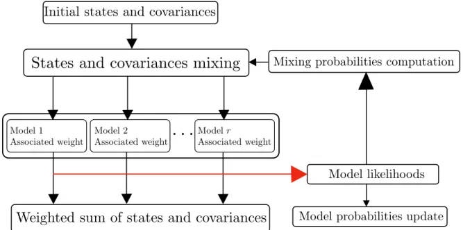
3.4.2 Interacting Multiple Model Filter (IMM) . . . 39
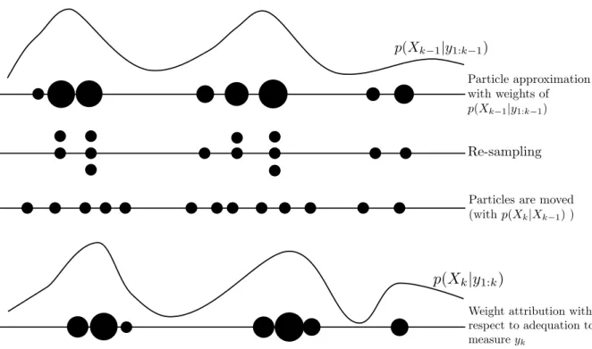
3.4.3 Non-linear filters . . . 40
3.5 IEKF applied to the 2D Frenet-Serret model . . . 46
3.5.1 Position observations in Cartesian coordinates . . . 48
3.5.2 Range and bearing observations . . . 49
3.5.3 Comparison with an EKF derived from the same target model . . . 50
3.5.4 Discussion . . . 51
3.6 IEKF applied to the 3D Frenet model . . . 52
3.6.1 Similarities with the Invariant theory . . . 52
3.6.2 Derivation of the algorithm . . . 53
3.6.3 Discussion on the filter’s expected stability . . . 55
3.7 Simulations . . . 55
3.7.1 2D simulations and comparison with the EKF on the same target model . . . 56
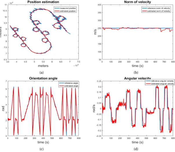
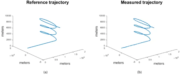
3.7.2 3D simulations . . . 56
3.8 Left-invariant UKF on a 2D model . . . 61
3.8.1 Derivation of the filter . . . 61
3.8.2 Results . . . 63
3.9 Conclusion. . . 63
4 Comparison with other existing algorithms and models 65 4.1 Résumé en français : Comparaison avec d’autres modèles et algorithmes existants . 66 4.2 Introduction . . . 66
4.3 Process noise tuning . . . 67
4.3.1 Issues of noise tuning . . . 67
4.3.2 Castella noise tuning . . . 69
4.4 Test on a real scenario . . . 71
4.5 The models and algorithms used for comparison . . . 72
4.5.1 Constant velocity and the EKF . . . 72
4.5.2 Multiple model and the IMM . . . 72
4.5.3 The Frenet-Serret target model with an IEKF . . . 72
4.5.4 The Frenet-Serret target model with an EKF . . . 73
4.6 Set of trajectories . . . 73
4.6.1 Simulators . . . 74
4.6.2 Kinematic characteristics . . . 75
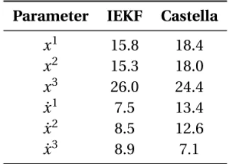
4.7 Results . . . 76
4.7.1 Set of trajectories to tune the process noise. . . 76
4.7.2 Set of trajectories to test the tunings . . . 77
4.8 Conclusion. . . 81
II Alternative state estimation: Smoothing 83 5 Smoothing applied to target state estimation 85 5.1 Résumé en français : Lissage appliqué à l’estimation d’état . . . 86
5.2 Introduction . . . 86
5.3 Smoothing as an estimation procedure for target tracking . . . 87
5.3.1 Smoothing as an alternative to filtering algorithms . . . 87
CONTENTS
5.3.3 Restriction to a deterministic evolution model over a sliding window as a
tun-ing strategy . . . 89
5.4 Smoothing applied to deterministic systems with random jumps. . . 91
5.4.1 Considered systems and simplifying assumptions . . . 91
5.4.2 Corresponding smoothing problem . . . 91
5.5 Proposed algorithm. . . 92
5.6 Application to a linear target model . . . 95
5.6.1 Target model. . . 95
5.6.2 Full resolution of the deterministic problem . . . 95
5.6.3 Linear target model with jumps . . . 96
5.7 Application to the 2D Frenet-Serret target model . . . 97
5.7.1 Solving the smoothing problem without jumps . . . 97
5.7.2 Accounting for jumps . . . 99
5.8 Comparison with other algorithms. . . 99
5.8.1 Comparison with the IEKF . . . 100
5.8.2 Comparison with an IMM . . . 101
5.9 Discussion . . . 105
5.9.1 Comparison with other filters. . . 105
5.10 Conclusion. . . 105
III Update rate adaptation 107 6 Update rate real-time optimisation 109 6.1 Résumé en français : Optimisation en temps réel de la fréquence des mesures . . . . 110
6.2 Introduction . . . 110
6.3 Fixed update optimisation criterion . . . 111
6.3.1 General formulation of the optimisation problem . . . 111
6.3.2 Resolution . . . 112
6.3.3 Practical use of the criterion . . . 114
6.4 Discussion . . . 114
6.5 Conclusion. . . 114
7 Adaptive update rate 117 7.1 Résumé en français : Cadence adaptative . . . 118
7.2 Introduction . . . 118
7.2.1 Links with prior literature . . . 119
7.2.2 Organisation and contributions of the chapter. . . 119
7.3 Update rate adaptation with a non-linear model. . . 119
7.3.1 Method: an adaptive criterion for update rate adaptation . . . 120
7.3.2 Underlying search strategy . . . 120
7.4 Application: Non-linear target model . . . 121
7.5 Experiments . . . 122
7.5.1 Tracking results with a Linear Kalman filter and an IEKF . . . 122
7.5.2 Update rate adaptation . . . 126
7.6 Discussion . . . 129
7.7 Conclusion. . . 129
8 Conclusion 131 8.1 Résumé en français . . . 131
8.2 Summary of the main contributions of the thesis . . . 131
CONTENTS
A Mathematical definitions: Lie groups 135
A.1 General definitions . . . 135
A.2 Specific Lie groups used in the thesis . . . 135
A.2.1 Group of 2D rotations SO(2) . . . 135
A.2.2 Group of 2D rotations and translations SE(2) . . . 136
A.2.3 Group of 3D rotations SO(3) . . . 136
A.2.4 Group of 3D rotations and translations SE(3) . . . 137
B More details about the Kalman Filter 139 B.1 Maximum Likelihood Estimator . . . 139
B.2 Algorithm derivation . . . 139
C Linearisation of the 2D Frenet-Serret model for smoothing 141 D Particle filters with jumps 143 D.1 The Rao-Blackwell particle filter . . . 143
D.1.1 Description . . . 143
D.1.2 Results on piecewise linear trajectories . . . 145
Chapter 1
Introduction
Sommaire 1.1 Résumé en français . . . . 2 1.2 Foreword . . . . 3 1.3 Radar systems . . . . 3 1.3.1 History . . . 31.3.2 General description of radar systems . . . 3
1.3.3 Digital processing. . . 5
1.3.4 Target tracking . . . 5
1.4 Motivations and objectives . . . . 7
1.4.1 State estimation. . . 7
1.4.2 Update rate adaptation . . . 7
1.5 Contributions of the thesis . . . . 8
1.6 Papers published during the thesis . . . . 8
CHAPTER 1. INTRODUCTION
1.1 Résumé en français
Ce travail est le résultat de trois années de thèse CIFRE-Défense menée avec Thales Land and Air Systems, et l’école des Mines ParisTech et en partie financée par la DGA (Direction Générale de l’Armement).
Le mot radar est l’acronyme anglais de "RAdio Detection And Ranging", et est apparu en 1940. L’histoire du radar remonte pourtant au début du vingtième siècle, avec les expériences de Nikola Tesla et de Christian Hülsmeyer. Cependant, les principales avancées des systèmes radars ont eu lieu avec la demande militaire dans les années 1930. Les radars modernes n’ont cessé de se développer depuis lors. Ces radars modernes sont des radars à compression d’impulsion, et ont mené aux radars à balayage électronique actuels. La théorie radar comprend de multiples champs de recherche, comme par exemple la théorie des antennes, le traitement du signal, le traitement numérique. Le travail présenté dans ce document traite principalement du traitement numérique, et notamment de la conception d’algorithmes dédiés aux besoins actuels en termes de perfor-mances de suivi de cibles, et de capacité de charge des radars.
Un radar envoie des ondes électromagnétiques dans l’espace et analyse les ondes réfléchies par les objets présents dans son champ de vision. Notamment, la position de la cible peut être connues en coordonnées (distance, azimut, élévation), correspondant aux mesures effectuées par le radar. Ces mesures n’étant pas infiniment précises, il est nécessaire de tenir compte du bruit de mesure, dont on connaît les caractéristiques dans ce système de coordonnées. Le pistage de cible consiste alors à former des "pistes" à partir de ces mesures de position bruitées. Une piste correspond à la trajectoire d’un objet d’intérêt, accompagnée de caractéristiques calculées par le radar, comme par exemple la cinématique de la cible considérée (vitesse, accélération, ...). Dans cette thèse, on s’intéresse à la phase d’estimation de l’état cinématique des cibles. On cherche donc à estimer des paramètres cinématiques choisis à partir de mesures de position bruitées, dans le but de prédire la position de la cible pour la poursuite active, qui nécessite d’orienter le faisceau du radar spécifiquement vers la cible que l’on veut suivre.
Les motivations de ce travail sont multiples. D’une part, de nouveaux types de radars voient le jour, notamment les radars multifonctions à panneaux fixes. Ces radars doivent faire face à de multiples tâches en parallèle. Un gestionnaire de ressources est donc utilisé afin d’ordonner les différentes tâches. Mais chacune des tâches doit également être optimisée en temps de façon à permettre au radar d’effectuer un maximum de tâches. Une partie du travail a donc été consacrée à la recherche d’une méthode pour optimiser le temps utilisé par l’antenne radar pour effectuer la poursuite active. D’autre part, les menaces ont également évolué. En effet, les cibles sont de plus en plus manœuvrantes, et peuvent avoir des accélérations, notamment normales, supérieures à 15g . Du côté des applications civiles, les drones représentent une menace, avec des comporte-ments différents des cibles usuelles traitées dans le cadre du contrôle de trafic aérien. Les solu-tions de pistage utilisées actuellement ne sont pas entièrement satisfaisantes pour ces nouvelles menaces, il s’agit donc dans la thèse de proposer d’autres méthodes pouvant répondre de façon plus adaptée aux problèmes de pistage des cibles hyper-manœuvrantes.
Les contributions de la thèse peuvent donc se résumer aux points suivants :
• Modèle de cible : un nouveau modèle de cible est proposé dans ce document. Ce modèle est exprimé en coordonnées intrinsèques, et est conçu pour représenter tous les mouvements possibles d’un objet en 2D ou en 3D.
• Algorithme de filtrage : l’espace mathématique utilisé pour décrire le modèle de cible étant différent des espaces vectoriels habituels, un algorithme de filtrage tirant parti de la formu-lation du modèle est développé. La formuformu-lation de cet algorithme est proche de celle du filtre de Kalman, et le filtre peut donc être implémenté assez facilement sur des simulateurs de pistage existants.
• Algorithme de lissage : afin de prendre en compte des sauts importants dans la dynamique des cibles, un algorithme reposant sur l’optimisation et spécialement conçu pour les
mod-CHAPTER 1. INTRODUCTION
èles à sauts est proposé. L’algorithme de lissage ainsi obtenu détecte les sauts très rapide-ment, et permet une convergence rapide de l’estimation après un saut.
• Cadence adaptative : cette contribution est indépendante des précédentes, et propose une méthode d’optimisation de la cadence de mesure de pistage, dans le but de réduire le temps du radar consacré à cette tâche.
• Expériences industrielles : des expérimentations de l’algorithme de filtrage présenté ont été réalisées dans différentes équipes de Thales. Ces résultats sont partiellement présen-tés dans ce document, et conduisent également à une discussion sur l’enjeu du réglage de paramètres des différents algorithmes.
1.2 Foreword
This work has been done in collaboration between Thales Land and Air Systems, the Ecole des Mines ParisTech PSL University, and has been partly supported by the DGA (Direction Générale de l’Armement), part of the French defence ministry. The main application of the work is ground and naval radars. In this introduction, the general principles of radar systems are presented, to have an overview of the main issues addressed in this work. The objectives and the main contributions of the thesis are presented. Finally, the organisation of the document is outlined.
1.3 Radar systems
1.3.1 History
The word Radar is an acronym for Radio Detection and Ranging. For a full introduction to the history of radar, please refer to [41] or to [17]. The word appeared in 1940 in the US army, it was in fact a code name. However, radar systems have begun to emerge much earlier. The earliest radar systems were developed to detect objects, without their participation, to avoid collisions for navigation purpose in the early 20th century. First experiments have been held by Nikola Tesla in 1900 and Christian Hülsmeyer in 1904. Yet, the main advances in radar systems are due to the military requirements of the 1930s, and of the second world war. Several countries developed their own radar systems simultaneously.
The modern radars have been developed in the second part of the 20th century. These modern radars are pulse compression radars. Their development have led to nowadays radars, such as scanned array radars. There are now very different types of radars, bistatic or monostatic radars, active or passive radars, primary or secondary radars. These radars have different use, including both military and civilian (for air traffic control) applications.
Radar theory deals with different scientific fields. Antenna theory, signal processing, digital processing, including algorithm design, statistical analysis are the main scientific domains that are used to design a complete radar system. This work is mostly concerned with digital processing, however, some fundamental notions about radar systems are necessary to understand the ins and outs of the applications developed in this document. They are briefly presented thereafter. 1.3.2 General description of radar systems
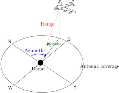
Numerous books are dedicated to radar, such as [41] or [105], and provide a thorough description of radar systems. A radar sends electromagnetic waves in the air. The wave is reflected when it encounters an object, as represented by figure1.1. The radar can then analyse the reflected signal. The radar is thus composed of a transmitter and a receptor that are responsible for the creation and the analysis of the electromagnetic wave.
The design of the antenna and the transmitted signal have to be carefully devised, since the signal is polluted with noise in the atmosphere, and the reflected signal has a very lower amplitude
CHAPTER 1. INTRODUCTION
Figure 1.1 – Radar fundamental principle
than the transmitted one, depending on the distance of the object. The energy of the received signal is proportional to the energy of the transmitted signal divided by the distance to the power 4. The receptor is thus very sensitive, and amplifies the received signal, but also adds some noise to it, due to the processing applied.
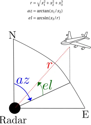
The primary radars measure the position of the target without any cooperation of the target. The position is usually given as the range (distance from the target to the radar), the azimuth of the target with respect to the radar, and the elevation of the target. Azimuth and elevation are angles. The range, azimuth and elevation coordinates are represented on figure1.2.
Figure 1.2 – Radar measurements
The range measurement is done by measuring the time the wave takes to go back and forth. This time is then multiplied by the velocity of the wave propagation, assumed to be the light veloc-ity, and divided by two (to take into account the round trip). The angle measurements (azimuth and elevation) are possible because of the directivity of the beam of the radar. The radar sends energy in a given direction, and the measured azimuth and elevation thus lie in a limited angle. This measurement is results in a lesser precision in the final position measurement than the range measurement, and the precision is degraded with the distance of the target to the radar, as will be developed in the radar measurement models in section2.5.
The secondary radars do not measure directly the position of the target. They ask for the pres-ence of a target, and for its position, and wait for the target answer. The target itself measures its own position. Secondary radars information relies on cooperation. This is the case (most often) for civilian traffic control, but not for military surveillance. Even for civilian applications, a
non-CHAPTER 1. INTRODUCTION
cooperative handling must be performed just in case. The advantage of using secondary radars is the greater precision of the measurements, especially for the altitude information. Secondary radars are also able to receive ADS-B (Automatic Dependent Surveillance - Broadcast) data from an aircraft that provides extensive information about its state, among which its position.
1.3.3 Digital processing
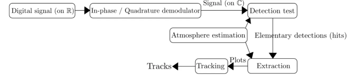
The digital processing unit receives raw information from the receptor. The digital processor is in charge of creating the plots, which are objects that represent a detection, with a radar observation associated to it. A plot represents one object, with diverse attributes, which may include its posi-tion, identificaposi-tion, the uncertainty of the measurement, the Doppler measurement, and possibly other useful information.
The atmosphere estimation is used to evaluate the level of noise present in a scene (for ex-ample, the presence of clouds in the sky can bring some noise to the signal). The detection test is a logical test of Neyman-Pearson, which is done thanks to a threshold. The Neyman-Pearson test consists of setting the false alarm probability and maximising the detection probability (this is possible because statistical noise models exist). The elementary hits correspond to zeros or ones that indicates the presence or not of an object (or part of an object).
Figure 1.3 – Digital processing
The signal received is digitised on an intermediate carrier (onR). Then, several treatments are applied to process the data and convert it into the description of one detection of one phys-ical object (indeed, a single object is illuminated by several elementary signals, that have to be agglomerated). The elementary treatments are summarised on figure1.3.
1.3.4 Target tracking
The radar can operate two different tasks: search and tracking. Search consists of detecting the presence of objects and reporting the detections. Tracking has to follow a given object, which is labelled, and infer its kinematic parameters.
The tracker then has to generate tracks from the plots. A track corresponds to the evolution of one given detected object in time. The observations are polluted by noise. There are two types of uncertainties: first the presence or not of an object of interest, when a detection does not cor-respond to such an object, it is called false alarm; and second, the uncertainties on the measure-ments, created by the radar itself. Indeed, the observations are not infinitely precise, and the val-ues are polluted by some noise, that must be estimated (it depends on the radar used), and this noise has to be taken into account in the algorithms. The noise comes from different factors, as explained in [40]. There is a part of the error dependent on the signal-to-noise ratio, a random part due to the noise in the final steps of the receiver (but it leads to relatively small errors, and gives mostly a limit on the achievable precision), some bias can be due to the calibration and measure-ment steps, some errors are due to propagation or uncertainties in the correction of propagation errors, and finally errors due to interferences or clutter are also present. Usually, only the first source of error (dependent on the signal-to-noise ratio) is modelled in the observation equation.
The objective of tracking is to analyse the plots, and output the tracks. A track contains the label of the object, some kinematic description (position, velocity ...), possibly the identification of
CHAPTER 1. INTRODUCTION
the object (aircraft, missile, boat for instance), and other useful information for the radar operator. Some of this information is directly output for the operator, and the rest is only used to feed the tracker. The chain for tracking is represented on figure1.4.
Figure 1.4 – Tracking chain
A track has first to be initialised. This is done during the initialisation phase, and the initial values of the kinematic parameters are computed, with their covariance. The association is the step where the plots are associated to the existing tracks. Indeed, assume there are at one point 6 identified tracks. The extractor gives a plot to the tracker. This plot has to be either associated to one of the 6 tracks, or considered as false alarm. This is the role of the association. The filtering part corresponds to the estimation of the different useful kinematic parameters of one track (for instance position, velocity, or acceleration ...). Finally the beam scheduler manages the order of the tasks that must be done, as detailed in the following. When the track is lost for several time steps, which means the radar cannot recover sight of the target, the track is killed.
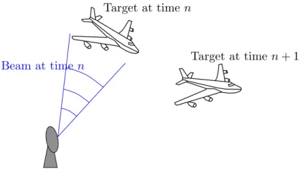
There are two modes in which the tracking can be done. The first mode is the track while scan mode (TWS). It is used to perform tracking during the search task. The second mode is Active Tracking (AT). It consists of dedicating the illuminations for one target. This mode can be used when the targets are menacing. The radar beam is oriented specifically in the direction of the target. The beam is thinner, so that the position measurement is more precise. This means that the radar has to know in which direction it should send its beam to find the target. The role of tracking is then both to tell the radar this direction, as shown on figure1.5, and estimate the kinematics of the target.
Figure 1.5 – Active track
If the radar antenna is non-rotating, the rate of the measurements can be made fully adaptive, in this case, the update rate adaptation for active tracking is part of the beam scheduling. The update rate is computed by the filtering algorithm, which tells the beam scheduler at what time the target should be next illuminated. The scheduler has to decide which task to perform in which order. There might be several targets in the active track mode, and the track while scan mode has to have enough time budget to detect any target that enters the sight of the radar. Moreover, in case of losses in detection, reacquisition beams or reacquisition patterns are scheduled.
CHAPTER 1. INTRODUCTION
1.4 Motivations and objectives
New types of radars are arising, and specifically fixed antenna, multifunction radars. This new gen-eration of radars require new algorithms, for two reasons. The first one is a necessity, since these radars are designed to perform several tasks in parallel. As concerns the tracking, the surveillance task and the active tracking tasks have to be done simultaneously (almost). This requires a careful management of the tasks the radar has to achieve. To do that, a resource manager (or a sched-uler) is used. But each task has to be optimised in itself, in order to save the radar’s time budget. The second reason is the new possibilities they offer. Indeed, the observations of the radar are no longer conditioned by the rotation of the antenna, so the observations update rate can be more easily adapted.
Another change in the environment of both military and civilian radars is the evolution of the threats. For the civilian application, drones are becoming more and more present in the air, and the airports are already faced with a drone problem. Indeed, their kinematics are different from the other targets, and there will also be the challenge to track a lot of targets at the same time. In the military world, the targets are becoming always more threatening, adopting unpredictable motions and manoeuvres to make the tracking fail and the radar lose the track.
In this context, new hyper-manoeuvring targets have emerged. Those targets can have accel-erations higher than 15g, that cannot be supported by pilots in an aircraft, even during a few tenth of seconds. This concerns mostly missiles that can have really any kind of motion. The tracking solutions used in the radars nowadays are not always satisfying against these targets. In particular, the state estimation task has to be thought over again.
1.4.1 State estimation
State estimation consists of estimating the main kinematic parameters of a target, thanks to partial observations. The radar observes the position of the target, the state estimator will have to predict and estimate the position, but also the velocity, or the acceleration if needed. For active tracking, the state estimation has to be fairly precise, because the challenge is to guide the radar beam for the next observation, to make sure not to lose the target.
Usually, in radar applications, the state estimation is performed using a filtering algorithm, such as the Kalman filter. One of the main objective of the thesis is to provide a state estimation method that is robust, precise, and that is able to keep track of highly-manoeuvring targets.
We identified several drawbacks of the target models usually used in industry, or developed in the literature to tackle the specific problem of estimating the state of highly-manoeuvring targets. These elements will be developed in detail within the document. Briefly, the models tend to be very simplistic, and do not allow enough degrees of freedom for the motion of the target, the chal-lenge was to build a target model which is also very simple, but that is more general and able to consider more class of targets and manoeuvres.
1.4.2 Update rate adaptation
The other task was to provide an update rate adaptation method that is efficient with the proposed estimation algorithm. The role of update rate adaptation is to minimise the radar load for the Active Tracking task. Indeed, to let the radar have enough time for all the tracks in AT, and for the surveillance, the duration for each task has to be optimised.
An adaptation algorithm is already used, but it is in fact not really adapted to the state estima-tion algorithms that are commonly adopted. The challenge is then to build an algorithm that is general, and that is suitable for all state estimation algorithms.
CHAPTER 1. INTRODUCTION
1.5 Contributions of the thesis
The work has led to contributions both for the state estimation task in itself, and for the adaptation of the update rate.
Target model The present work proposes a novel target model, expressed in intrinsic
coordi-nates. This target model is designed to represent the possible motions of the target directly in its local frame. It uses the Frenet-Serret frame, which can describe any curve in the 2D or the 3D space. Indeed, it appears that the targets very often follow piecewise constant motions, which means that the commands that are applied to it are piecewise constant. The model is meant to represent these commands in the best possible way.
Filtering algorithm The state estimation methods usually applied to other target models are not
appropriate for the one we propose. A new filtering algorithm is created to perform filtering for our target model. This algorithm is designed as a geometric version of the extended Kalman filter, and easily implementable for industrial applications.
Smoothing algorithm To account for jumps in the dynamic features governing the target motion
such as acceleration or jerk, and to consider accurately the fact that the command parameters may often be modelled as piecewise constant, an optimisation based smoothing algorithm has been constructed for the 2D target model. This smoothing algorithm has the ability to detect jumps in the motion and to react very rapidly when a jump occurs, so that the estimation converges faster after the jump.
Update rate adaptation Besides the preceding contributions related to filtering, this work
pro-poses a new update rate adaptation algorithm that is compatible with any target model. The new algorithm is designed to be very general, and can cooperate with all the estimation algorithms that are presented in this document (the algorithms developed in this work, but also the ones presented as bibliographic references).
Industrial experiments Experiments have been done with Thales, in several teams coordinated
by a working group on tracking, both for civilian and military applications on real tracking simula-tors, a result on a real trajectory is presented in this document. Some other extensive experiments with other algorithms on several different simulated trajectories have been done and the results are also presented in a separate chapter. A discussion on the tuning issue is presented, since it has been one of the major subject of discussion when the algorithm was presented and tested in the different teams.
1.6 Papers published during the thesis
Several publications have been made during this thesis. They are listed here, with the following corresponding chapters:
Conference papers:
• Pilté, M., Bonnabel, S., Barbaresco, F. (2017, June). An innovative nonlinear filter for radar kinematic estimation of maneuvering targets in 2D. In Radar Symposium (IRS), 2017 18th International (pp. 1-10). IEEE, [94]. This paper presents the 2D Frenet-Serret target model, with the 2D Invariant Extended Kalman Filter (IEKF) applied to target tracking, results can be found in chapter2and3.
CHAPTER 1. INTRODUCTION
• Pilté, M., Bonnabel, S., Barbaresco, F. (2017, November). Drone Tracking Using an Innova-tive UKF. In International Conference on Geometric Science of Information (pp. 301-309). Springer, Cham, [93]. This paper exposes an extension of the IEKF with the 2D Frenet-Serret target model, with the use of the update step of an Unscented Kalman Filter adapted to the Lie group space. Results can be found in chapter3.
• Pilté, M., Bonnabel, S., Barbaresco, F. (2017, December). Tracking the Frenet-Serret frame associated to a highly maneuvering target in 3D. In Decision and Control (CDC), 2017 IEEE 56th Annual Conference on (pp. 1969-1974). IEEE, [91]. This paper presents a 3D target model based on the Frenet-Serret frame, with the IEKF algorithm to perform estimation. Results can be found in chapters2and3.
• Pilté, M., Bonnabel, S., Barbaresco, F. (2018, June). Maneuver Detector for Active Track-ing Update Rate Adaptation. In 2018 19th International Radar Symposium (IRS) (pp. 1-10). IEEE, [95]. This paper proposes a manoeuvre detector based on a particle filtering algorithm designed to track kinematic jumps in the trajectory. This paper was not reproduced in this document.
Journal papers:
• Pilté, M., Bonnabel, S., Barbaresco, F. (2018). Fully-Adaptive Update Rate for Nonlinear Trackers. IET Radar, Sonar & Navigation, [90]. This paper explores the update rate adap-tation problem to optimise the radar load for active tracking. The results can be found in chapters6and7.
• Pilté, M., Bonnabel, S., Livernet, F. A novel nonlinear least squares approach to highly ma-neuvering target target tracking. Submitted upon invitation to Comptes Rendus Physique (Elsevier-Académie des Sciences), 2018. This paper exposes a new method for target track-ing, based on a modified smoother that tracks jumps. The results are explained in chapter 5.
1.7 Organisation of the document
This document is organised in three parts:
• Part I focuses on state estimation. The construction of a new target model in intrinsic co-ordinates, adapted to nowadays manoeuvring targets, is presented in chapter2. This target model is expressed in 2D and in 3D. The two models designed in this chapter will be used throughout the entire document. Then, a filtering algorithm that is adapted to this target model is derived in chapter3. Firsts results on toy examples are presented. Some extensive tests and comparison with other commonly used target models and filtering algorithms are also presented in chapter4.
• Part II introduces an estimation method that has not been much used in the radar com-munity: smoothing. We take inspiration from the use of optimisation based smoothing methods that have become prevalent in the robotics community for robot localisation and mapping since the beginning of the 2010s. In this work, we have applied it to radar target tracking, and modified the algorithm to suit the problem of tracking manoeuvring and un-predictable targets. A smoothing algorithm is presented, first for a linear target model, and then applied to the 2D target model derived in Part I. This smoothing algorithm is more specifically constructed to track kinematic and/or dynamic jumps in the motion of the tar-gets, to be able to provide accurate estimations right after the jumps.
• Part III is dedicated to the update rate adaptation problem. The algorithm of Blackman and Van Keuk, used in industry, is first pedagogically and thoroughly explained in chapter6. We
CHAPTER 1. INTRODUCTION
thus point out the approximations that were made in their paper [108]. Then a more general algorithm is derived in chapter7. This algorithm is compatible with any filtering algorithm or target model, and experiments show that the radar load is lower using this new algorithm. Finally, a synthesis of the work and a discussion on possible future leads are presented in the conclusion of the document, in chapter8.
Part I
State estimation: target models and
filtering algorithms
Chapter 2
Target model in intrinsic coordinates
Sommaire
2.1 Résumé en français : Modèle de cible en coordonnées intrinsèques . . . 14
2.2 Introduction . . . 14
2.3 State of the art . . . 16
2.3.1 Model without manoeuvres . . . 16 2.3.2 Manoeuvre models with decoupled coordinates. . . 17 2.3.3 Non-linear models, intrinsic models. . . 20 2.3.4 Models with jumps . . . 21 2.3.5 Lie group based models . . . 22 2.4 Radar industrial tracking models . . . 23
2.4.1 3D target model . . . 23 2.4.2 Multiple target models . . . 23 2.5 Radar measurement models . . . 25
2.6 New target model in intrinsic coordinates . . . 27
2.6.1 2D target model . . . 27 2.6.2 3D target model . . . 29 2.6.3 Generalisations . . . 31 2.7 Conclusion . . . 32
CHAPTER 2. TARGET MODEL IN INTRINSIC COORDINATES
2.1 Résumé en français : Modèle de cible en coordonnées intrinsèques
L’estimation d’état nécessite deux composants principaux : un modèle d’évolution de cible d’une part, et un algorithme de filtrage (ou d’estimation en général) d’autre part. Ce chapitre est dédié à l’élaboration d’un modèle adapté aux cibles hyper-manœuvrantes. D’une façon générale, on peut identifier trois grands types de modèles de cible :
• Les modèles linéaires, qui sont aussi les plus simples, peuvent être en 2D, ou en 3D, et de dimension variée dans l’état (modèle linéaire de vitesse, ou d’accélération, ou de jerk ...). • Les modèles non-linéaires plus complexes, qui décrivent des mouvements plus complexes,
comme des virages coordonnés par exemple.
• Enfin, les modèles à sauts, qui permettent de décrire des trajectoires qui ont une com-posante discontinue (par exemple avec des sauts de vitesse ou d’accélération), ou des tra-jectoires avec des sauts entre modèles.
Il est aussi nécessaire de définir le modèle de mesure, permettant de relier les mesures radar à l’état du système. Souvent, il se résume à donner les équations de passage du repère des mesures radars (distance, azimut, élévation) au repère cartésien fixe dans lequel est exprimé la position de la cible dans l’état. On y ajoute un bruit Gaussien pour modéliser l’imprécision des mesures radar. Le modèle de cible proposé dans cette thèse utilise le repère de Frenet-Serret, qui permet de décrire n’importe quelle trajectoire en 2D ou en 3D. Le modèle de cible a donc été développé en 2D et en 3D. Deux hypothèses communément admises sont également appliquées pour établir le modèle : d’une part, la cible ne glisse pas (on appelle cette hypothèse la contrainte non-holonome), c’est-à-dire que le vecteur vitesse de la cible est toujours colinéaire au vecteur tangent du repère de Frenet-Serret. D’autre part, on fait une hypothèse sur la cinématique de la cible, dans notre cas, on suppose que la norme de la vitesse, la courbure et la torsion de la trajectoires sont (presque) con-stantes. Cette seconde hypothèse peut être légèrement relâchée et remplacée par une hypothèse d’évolution linéaire. Cependant, il n’est pas toujours intéressant de complexifier les équations du modèle car cela rend le problème d’estimation plus difficile. Le modèle ainsi obtenu est parti-culièrement adapté aux virages, contenus dans un plan ou non. C’est une des particularités de ce modèle par rapport à d’autres modèles de virages : il peut décrire un virage avec de la torsion (dans le cas 3D). Du bruit blanc peut être rajouté au modèle afin de tenir compte des écarts en-tre la réalité et le modèle construit. Ce modèle a une forme particulière, due à la présence de la matrice du repère de Frenet-Serret dans la formulation de l’état. L’état est donc partiellement à valeurs dans le groupe de Lie SE(2) pour le cas 2D, ou SE(3) pour le cas 3D, et partiellement dans l’espace vectorielR2ouR3. Le modèle nécessite donc une adaptation des algorithmes de filtrage traditionnels, c’est l’objet du chapitre suivant.
2.2 Introduction
To perform state estimation, two main components are needed: a target evolution model, and an estimation algorithm, based on this model an on the radar observations. In this chapter, we concentrate on the target model. The model describes the possible motions of a target, considered as a point object, in space. For example, an overview of missile motion equations is given in [104]. The most basic motion comes from Newton’s laws, which can lead to complex equations, specific to one category of targets. However, to perform state estimation, we seek the simplest models as possible, that take into account a large class of targets. The model has to be simple enough, so that the estimation problem is kept tractable. Indeed, very high derivation orders of the position are very difficult to estimate because the radar only measures the position of the target, polluted by noise (and sometimes the Doppler velocity), so variables coming from complex equations are difficult to estimate. However, if the model is too rigid because of its simplicity, and does not allow enough degrees of freedom in the motion of the target, the estimation algorithm might not be able
CHAPTER 2. TARGET MODEL IN INTRINSIC COORDINATES
to keep the track, because of the lack of adequacy between the model and the real trajectory. This can lead to divergence or very poor precision. The difficult part when designing a target model is thus to find a balance between the simplicity and the universality of the model.
The quality of the target model and its adequacy to the real movement are decisive for the tracking. The target models possibilities are virtually infinite. In this chapter, we list the ones that seem most pertinent, and we group them into different categories:
• The simplest models are the linear models, that can be formulated in 2D, in 3D, and of in-creasing dimension (linear model of velocity, of acceleration, of jerk, ...).
• There are more complex non-linear models, that account for more complex motions, such as coordinated turns.
• Finally, the jumping models can account for trajectories that have a discontinuous compo-nent (for instance that have jumps in the velocity or in the acceleration).
To describe the target evolution and derive the so-called target and measurement models, we use a state space representation. The targets are considered as point objects, and target models describe the motion of a point moving in space. This is a general setting in which the state Xt∈ Rn
is the solution of a stochastic differential equation, and can be defined as one realisation of the underlying stochastic process, so it is an element of a vector space (or an element of a more general space, as we will see later), and the observation is a vector yt∈ Rm, and the equations write
˙
Xt= f (Xt, ut, wt) (2.1)
yt= h(Xt, ut, vt) (2.2)
where utis an input vector, f is the evolution function, h is the measurement function, wt, vtare
independent white Gaussian noises. wtis called the process (or model) noise, and vtis called the
observation (or measurement) noise. The process noise is used to compensate for the differences between the model and the real trajectory of the target. The observation noise is used to model the imprecisions of the radar measurement process. Usually, the noises are chosen to be additive, because it is more convenient for the state estimation algorithm.
Nowadays, the air defence radar industry is facing new challenges with ever increasingly ma-neuvering targets. Some targets can reach Mach 8 velocities with 30g accelerations, and this will increase even more in the future years. The target models that are currently used are not always entirely satisfactory when it comes to track these targets, and new models have to be designed. A way to inject some structure through a motion model into a trajectory that is deliberately trying to make the radar lose track of it, is to resort to physical considerations: the changes in aerodynamic lift and thrust-drag accelerations are limited, and those accelerations can in fact be expected to be piecewise nearly constant.
In the present work, we propose, as a very simple geometric model, to use the Frenet-Serret frame to describe the motion and to assume nearly constant curvature and torsion. This model includes helical motions that are particularly challenging to track. Our model can be related to [31], [16], or more recently [32].
Target models can be expressed either in continuous or in discrete time. In this chapter, we will use one or the other. The discretisation of continuous models is usually quite simple and straightforward, or the estimation algorithms can accommodate a continuous target model. It is also quite widespread to describe the target evolution in continuous time. The radar measurement model is always expressed in discrete time. In this case, we have Xn= Xtn in the measurement
equation.
This chapter first presents the most well-known target models in literature in section2.3, and class them into categories, and the target models widely used in industry are detailed in section 2.4. Then, the radar measurement model is described in section2.5, and finally the target model created during this thesis is developed in section2.6.
CHAPTER 2. TARGET MODEL IN INTRINSIC COORDINATES
In this work, the state will be denoted by Xt ∈ Rn for the continuous time or Xk ∈ Rn for the
discrete time, where n is the dimension of the state. The measurements will be denoted yk ∈ Rp,
where p = 2 or 3, depending on the dimension of the measurements (2D or 3D). The cartesian position is denoted by x =¡x1 x2 x3¢T
.
2.3 State of the art
2.3.1 Model without manoeuvres
A point in space can be described by its position and velocity vectors. For example the vector Xt=¡xt1 x˙t1 x2t x˙2t x3t
¢T
can be used as a state vector in a Cartesian coordinate system. When the target is considered as a punctual object, the non-manoeuvring motion is described by the fact that the velocities along the first two coordinates x1and x2are constant, and that the velocity is
null for the x3coordinate. Indeed, in target tracking, we consider there is no manoeuvre when the
target stays in a horizontal plane, see [80]. So this means:
¨ xt1= 0 ¨ xt2= 0 ˙ xt3= 0
Usually, in practice this ideal equation is modified to add a white noise w (t ), that accounts for small unpredictable errors, such as turbulences. The equations then become
¨ x1t = 0 + wt1 ¨ x2t = 0 + wt2 ˙ x3t = 0 + wt3
The corresponding state space representation is given by: ˙
Xt= AXt+ Bwt (2.3)
where wt= [wt1, wt2, wt3]Tis a white continuous Gaussian noise, with
A = 0 1 0 0 0 0 0 0 0 0 0 0 0 1 0 0 0 0 0 0 0 0 0 0 0 , B = 0 0 0 1 0 0 0 0 0 0 1 0 0 0 1
The discrete time equivalent for this model is, see for instance [6]
Xk+1= FXk+ Gwk (2.4) where F = 1 T 0 0 0 0 1 0 0 0 0 0 1 T 0 0 0 0 1 0 0 0 0 0 1 , G = T2/2 0 0 T 0 0 0 T2/2 0 0 T 0 0 0 T (2.5)
and wk= [w1k, wk2, wk3]Tis a white discrete Gaussian noise and T is the sampling time. wk1and w2k
CHAPTER 2. TARGET MODEL IN INTRINSIC COORDINATES
If the coefficients of w are uncorrelated, the covariance matrix Q associated to Gw is
Q = q1T4/4 q1T3/2 0 0 0 q1T3/2 q1T2 0 0 0 0 0 q2T4/4 q2T3/2 0 0 0 q2T3/2 q2T2 0 0 0 0 0 q3 (2.6)
with q1, q2, q3the variances of w1, w2, w3respectively.
These models are known to be models with (almost) constant velocity. Adding non-essential components in the state vector (for instance the acceleration or the jerk) would add complexity in the model and decrease the performances for constant velocity trjectories.
2.3.2 Manoeuvre models with decoupled coordinates
The manoeuvres of a target are triggered by the control input u, which is most often unknown to the user. There are then two main solutions to tackle this problem:
• Input estimation: this consists in modelling the input as an unknown but deterministic pro-cess, that will be estimated along with the state during the estimation. Such methods are called input estimation methods, see for instance [20]. However, it is hard to model an un-known process, and it often amounts to estimating jumps and values of the input.
• Stochastic process: the other solution is to model the input as a stochastic process. This is more often used in practice, and it comes to using noise models. In the literature, there are three groups of methods:
1. White noise models: the control input added to the state evolution equation is mod-elled as a white noise. This includes constant velocity or acceleration models and poly-nomial models.
2. Markov process models: the control input is modelled as a Markov process, autocorre-lated in time. This includes the Singer model.
3. Semi-Markovian jumping models: the control input is modelled as a semi-Markovian process with jumps.
A lot of target models assume the coupling between the coordinates is low and can be ne-glected. It is the case for those for which the control input u is modelled as a random process. In the reminder of this section, the models will be presented in one dimension. The generalisation in 2D or 3D consists only in concatenating the directions x1, x2, x3to form one state vector.
Let x, ˙x and ¨x be the position, velocity and acceleration of a target in one dimension. We have: ¨
xt= at (2.7)
The possible definitions of at will lead to different target models, listed in this section. In the
following paragraphs, the state vector will always be X = [x, ˙x, ¨x]T.
Before going further, let us first give the definition of a stochastic process. This notion will be used several times in the sequel.
Definition 2.1. Stochastic process: it is a parametrised collection of random variables {Xt}t ∈T
de-fined on a probability space. A complete definition and examples are provided in [89]. An intuitive interpretation is to see a stochastic process as a mathematical object that represents the evolution of a random variable. A family of random variables (Xt)t ∈R+ is a continuous stochastic process,
(Xk)k∈Nis a discrete stochastic process. A basic example is the random walk.
The target state is the solution of a stochastic differential equation, and it is defined as one realisation of the underlying stochastic process.
CHAPTER 2. TARGET MODEL IN INTRINSIC COORDINATES
White noise acceleration model
The simplest model for a target manoeuvre is to consider a model with white noise acceleration. This model assumes that the acceleration of the target ¨x(t ) is only white noise, see [6]. This means that
a(t ) = 0 + w(t) or in other words
¨
x(t ) = 0 + w(t)
The acceleration is thus constant up to a white noise. The difference with the non-manoeuvring model is the level of the noise added: the white noise process w is used to model the effects of a manoeuvre (a switch from a given acceleration to another one for instance). A manoeuvre has the aim to achieve a task and is rarely independent of the state variables in time. The major appeal for this model is its simplicity. It is nonetheless used quite often in practice. This is also referred to as the (almost) constant velocity model.
Almost constant acceleration
The second simplest model is the acceleration model along a Wiener process, see [6]. It assumes the acceleration is a process with independent increments. It is also simply called the (nearly) constant acceleration model. This model has too widely used versions. The first one, the jerk model with white noise, assumes the derivative of the acceleration (the jerk) ˙at is an independent
process: ˙at= wt. The evolution equation is ˙Xt= AXt+ Bwt, where
A = 0 1 0 0 0 1 0 0 0 , B = 0 0 1
The discrete equivalent for this model is
Xk+1= F3Xk+ wk, F3= 1 T T2/2 0 1 T 0 0 1 (2.8)
The second version is the acceleration model of the Wiener sequence. The acceleration incre-ment is supposed to be an independent process. An acceleration increincre-ment on a time range is the integral of the jerk on this interval. This model is directly expressed in discrete time by
Xk+1= F3Xk+ G3wk, G3= T2/2 T 1 (2.9)
The models above are simple but rough. Real maneuvers have almost never almost constant accelerations that are decoupled along the different directions.
Polynomial models
Any target trajectory can be approximated by a polynomial with a given and known precision. It is thus possible to model the movement of the target by a polynomial of degree n in Cartesian coordinates: x1t x2t x3t = a0 a1 . . . an b0 b1 . . . bn c0 c1 . . . cn 1 t .. . tn/n! + w1t w2t w3t (2.10)
with a specific choice of coefficients ai, bi, ci, where (x1, x2, x3) are the position coordinates and
CHAPTER 2. TARGET MODEL IN INTRINSIC COORDINATES
These polynomials models, of degree n means that the n-th time derivative of the position is (almost) constant. Constant velocity or acceleration models described in the previous sections are particular cases of this model (for n = 1,2 respectively).
In the general case, this model does not seem very satisfying for the tracking application. This type of method is of better use when confronted to smoothing problems, when one needs to fit a smooth curve to a set of data. It is hard to design an efficient method to determine the coefficients ai, biand ciin the general case.
The Singer model
The white noise models presented earlier are the simplest class of random processes in time. An-other class contains the Markov processes, including Wiener processes and the white noises as particular cases.
The Singer model, fully explained in [103], assumes the acceleration of the target at is a
sta-tionary Markov process of zero mean. The Singer model is based on the assumption that the ac-celeration is an Ornstein-Uhlenbeck process. See for example [57] for a definition of the Ornstein-Uhlenbeck process. Indeed, this means that each coordinate of the acceleration a1, a2, a3 is an Ornstein-Uhlenbeck process and that the coordinates are mutually independent. We have:
˙
at= −αat+ wt,α > 0 (2.11)
with wt a continuous white Gaussian noise, and the autocorrelation of each acceleration
coordi-nate thus writes:
E[atiat +τj ] = δi jΣ2e−ατ
whereΣ is the acceleration noise standard deviation and 1/α is a manoeuvre time constant. Such a model accounts for the fact that accelerations in one direction tend to last for some time 1/α, but on average the acceleration of the target is 0. This gives the following discrete evolution equation (2.12) for each position coordinate, and between two time instants k and k + T:
xk+T= Fxk+ wk (2.12) with F = 1 T αT−1+eα2 −αT 0 1 1−eα−αT 0 0 e−αT
The process noise covariance matrix Q (from which the Gaussian white noise wkis drawn) writes
Qk = E[wkwkT]. The expectation can be explicitly computed as a time integral, as shown in the
Appendix I of [103], and finally the matrix writes
Qk= 2αΣ2 T5 20 T4 8 T3 6 T4 8 T3 3 T2 2 T3 6 T2 2 T
From equation (2.12), we see that:
1. When the manoeuvre duration constant 1/α increases to the infinity (which means that αT decreases), the Singer model becomes a constant acceleration model. This is normal since the deterministic part of the acceleration in the Singer model becomes constant whenτ goes to the infinity.
2. When 1/α decreases (which means that αT increases), the Singer model goes to the constant velocity model. In this case, the acceleration becomes a white noise.
CHAPTER 2. TARGET MODEL IN INTRINSIC COORDINATES
The Singer model is thus a mix of a (almost) constant velocity and (almost) constant accelera-tion model. It is thus more general than one or the other, and is more suited to track manoeuvring targets.
This is why this acceleration Singer model has become popular for target manoeuvre models, and has led to the development of update rate adaptation method, specifically designed for this model, see chapter6. It also led to the development of other target manoeuvre models.
The Singer target model is by construction an a priori model. Indeed, real time information about the target behaviour is not used to tune the model. The parameterΣ can be made adaptive. The adaptation is however limited because in the model, the acceleration has a zero-mean at each time instant. Indeed, for an a priori model, it is the natural approximation.
2.3.3 Non-linear models, intrinsic models Coordinated turn model
The constant turn model assumes the target undergoes a turn manoeuvre, with constant angu-lar velocity, and constant speed, in a 2D plane, see for instance [6], [87]. The state is defined to be Xt =¡x1t, ˙x1t, x2t, ˙x2t,ωt¢, whereω is the (constant) angular rate. The equations in continuous
representation are ˙ Xt= AXt with A = 0 1 0 0 0 0 0 0 −ω 0 0 0 0 1 0 0 ω 0 0 0 0 0 0 0 0
The discrete equation writes
Xk+1= FkXk (2.13)
with (ifω is not too small, otherwise a Taylor development can be performed):
Fk= 1 sin(ωωt) 0 −1−cos(ωt)ω 0 0 cos(ωt) 0 −sin(ωt) 0 0 1−cos(ωt)ω 1 sin(ωωt) 0 0 sin(ωt) 0 cos(ωt) 0 0 0 0 0 1
Of course as always, white Gaussian noise can be added to the evolution equation, to account for differences between the real motion and the model. This model is very useful in practice, as we will see for multiple models. When it is used as a single model, some significant noise should be added toω and to the velocity, to allow manoeuvres.
Intrinsic coordinate model
The simplest 2D intrinsic coordinate model considers the target as a point mass subject to two accelerations, one tangential, aT,tkand one normal, aN,tk, and to the current velocity, see [59]. The
accelerations are known. The continuous kinematic state of the target is described by its direction, θt(in the trigonometric way from the x1-axis), its velocity ˙st, and its cartesian coordinates x1t and
x2t. The state and parameter vectors thus are
Xt=¡x1t, x2t,θt, ˙st¢ T
utk = [aT,tk, aN,tk]
CHAPTER 2. TARGET MODEL IN INTRINSIC COORDINATES
The dynamics of the target are described by the usual differential equations for a curvilinear mo-tion: ¨ st= aT,tk ˙ st˙θt= aN,tk ˙ xt= ˙stcos(θt) ˙ yt= ˙stsin(θt)
These equations can then be integrated to get the corresponding discrete time target model. This model can of course be extended to lie in the 3D space, but it can also be augmented to avoid a degeneration problem due to the fact that all values of Xk cannot be reached. The accelerations
aT,tk, aN,tk are here supposed to be known, or measured, we will see in section2.3.4how they can
enter the state (or the estimation in general). 2.3.4 Models with jumps
Jump Markov linear systems
Jump Markov linear systems are linear systems with parameters that evolve in time according to a Markov chain, with a finite state space, as explained in [50]. Let rk, k = 1,2,... be a discrete time
Markov chain with known transition probabilities. A linear system with markovian jumps can be modelled in the following way:
Xk+1= F(rk+1)Xk+ B(rk+1)uk+1+ G(rk+1)wk+1 (2.14)
yk= C(rk)Xk+ A(rk)uk+ D(rk)vk (2.15)
where uk is a known input, and wkand vk are sequences of white Gaussian independent noises.
A jump Markov linear system can be seen as a linear system whose matrices (A(rk), B(rk), C(rk),
D(rk), F(rk), G(rk)) evolve in time according to a Markov chain with finite state space rk. Neither
the process Xknor the process rkare observed, only the noisy measurements yk are observed. rk
represents in fact pieces of trajectory, on which one model is true. So changes in the Markov chain (when rk6= rk−1) implies jumps in the trajectory from one model to another.
Variable rate models
In [32], [58] and [59], the authors have designed some models that take into account the temporal structure of a manoeuvring target trajectory. The variable rate models consider that the target motion is deterministic when it is conditioned by a sequence of change-points and manoeuvre parameters. It is similar to Jump Markov Linear Systems, except that we have non-linear equations (also possible for the latter), and more importantly, continuous time changes.
Tracking is the step where the kinematic state of a target is estimated (its position, velocity, . . . ) from a set of noisy or incomplete observations. The state of the target is continuous. How-ever, as we saw in the last section, a lot of tracking systems model the dynamics of a target as a discrete Markov process. This hypothesis is indeed quite simple: when the state is discretised at the instants of the observations, we come to consider a Hidden Markov Model (HMM), which can then be used to design a standard Kalman filter or a particle filter. HMM methods are explained in [34]. The drawback of such an hypothesis is that the dynamics of the system may not be as ac-curate as using a continuous-time model (the equations of motion of a continuous system being continuous in time).
The principle of variable rate models is the following: consider a general model from 0 to T, time between which some observations {y1, . . . , yN} are made at time instants {t1, . . . , tN= T}.
Dur-ing this time period, an unknown number of changes, K, occur at time instants {τ0= 0, τ1, . . . ,τK},
each change is associated to change parameters, {u0, u1, . . . , uK}. We assume the trajectory can be
CHAPTER 2. TARGET MODEL IN INTRINSIC COORDINATES
elements of a Marked Point Process (MPP). The hidden state is a continuous process called Xt.
Discrete sets containing multiple values will be called y1:n= {y1, . . . , yn}. The variable rate model is
an example of a hybrid dynamic system, used to model at the same time continuous and discrete behaviours.
The objective for inference will be to estimate the sequence of change-points until the current time tn:θn= {τj, uj, ∀j : 0 ≤ τj< tn}. It will also be useful to define a variable for the changes that
occur in the time interval [tn−1, tn) :θn\n−1= {τj, uj, ∀j : tn−1≤ τj< tn}.
To simplify the notations, let us introduce the following notations, to keep in mind the most recent changes:
Kt= max(k : τk< t )
Kn= K(tn)
The sequence of changes is supposed to be a Markov process: {τk, uk} ∼ p(uk|τk,τk−1, uk−1)p(τk|τk−1, uk−1)
Now, it is possible to write the a priori density for the sequence of changes, p(θn) and the extent
of the sequences p(θn\n−1|θn−1). The dynamics of the state is governed by a differential equation
which depends on the most recent change-point. ˙
Xt= f (Xt,τKt, uKt) (2.16)
With a new sequence {X0, X1, . . . , XK}, which is the value of the state at each change-point (i.e. xτk)
and assuming that an analytical solution exists, a transition function can be derived:
Xt= f (XKn, uKn,τKn, t ), τKn≤ t ≤ τKn+1 (2.17)
2.3.5 Lie group based models
These late years, work has been done to model the motion of objects with rigid transformations and the associated appropriate spaces. Especially in the robotic field, Lie groups have appeared to be the right spaces to describe the possible moves of a robot. Indeed, one of the most well-known Lie groups, SE(2), represents all possible translations and rotations in 2D. The definition of Lie groups and the main results used in this document are provided in appendixA. This thus appears the right frame to work in. The works of [10], or [36] are examples of Lie group models developed in robotics.
More recently, target models on Lie groups have emerged in the radar target tracking commu-nity. This includes the very recent (2018) work of [42]. In this paper, the authors use a coordinated turn target model, and show it can be embedded in a Lie group setting. The state is set to be Xk =¡xk θk ωk uk
¢T
, with xk the Cartesian position,θk the orientation of the target,ωk the
angular rate, and uk the translational speed. It can be represented in G = SE(2) × R2, with the
following 6 × 6 matrix: gk= cosθk − sin θk xk1 0 0 0 sinθk cosθk xk2 0 0 0 0 0 1 0 0 0 0 0 0 1 0 uk 0 0 0 0 1 ωk 0 0 0 0 0 1
The authors model then the dynamics with the following equation on Lie groups gk+1= gkexpG
¡