Detailed analysis of configuration interaction and calculation of radiative transition rates in seven times ionized tungsten (W VIII)

atoms

Article

Detailed Analysis of Configuration Interaction and Calculation

of Radiative Transition Rates in Seven Times Ionized Tungsten

(W VIII)

Jérôme Deprince 1 _{and Pascal Quinet} 1,2,_*

1 _{Astrophysique et Spectroscopie, Université de Mons, Mons B-7000, Belgium;}

E-Mail: jerome.deprince@gmail.com

2 _{IPNAS, Université de Liège, Liège B-4000, Belgium}

* Author to whom correspondence should be addressed; E-Mail: Pascal.quinet@umons.ac.be; Tel.: +32-65-373-629.

Academic Editor: Bastiaan J. Braams

Received: 21 May 2015 / Accepted: 23 June 2015 / Published: 30 June 2015

Abstract: A new set of oscillator strengths and transition probabilities for EUV spectral lines of seven times ionized tungsten (W VIII) is reported in the present paper. These results have been obtained using the pseudo-relativistic Hartree-Fock (HFR) method combined with a semi-empirical optimization of the radial parameters minimizing the discrepancies between computed energy levels and available experimental data. The final physical model considered in the calculations has been chosen further to a detailed investigation of the configuration interaction in this atomic system characterized by complex configurations of the type 4f14_5s2_5p5_{, 4f}14_5s2_5p4_{nl, 4f}14_5s5p6_{, 4f}13_5s2_5p6_,

4f13_5s2_5p5_{nl and 4f}12_5s2_5p6_{nl (nl = 5d, 6s).}

Keywords: atomic structure; oscillator strengths; transition probabilities; W VIII spectrum

1. Introduction

It is now well established that tungsten plays an important role in the development of fusion reactors (see e.g., [1–5]). Indeed, this element has been chosen to be the main component of the divertor of the International Thermonuclear Experimental Reactor (ITER) so that spectral lines of W ions sputtered from the wall to the core plasma provide a key information for plasma emission analysis

and diagnostic purposes. As a consequence, a detailed knowledge of the atomic structure and radiative properties of almost each ionization stage of tungsten is required. Over the past few years, several of our works were focused on the determination of spectroscopic data for neutral to moderately ionized tungsten. More precisely, oscillator strengths and transition probabilities were calculated for a large number of lines in W I [6], W II [7], W III [8], W IV [9], W V [10] and W VI [11]. In all these studies, the pseudo-relativistic Hartree-Fock (HFR) method including a large amount of intravalence and core-valence electronic correlation effects was combined with a semi-empirical process minimizing the discrepancies between calculated and available experimental energy levels. For W I, W II and W III, the accuracy of this approach was assessed through detailed comparisons with experimental radiative lifetimes measured with the time-resolved laser-induced fluorescence (TR-LIF) technique while, for W IV, W V and W VI, our new HFR results were supported by a detailed comparison with transition probabilities obtained using different theoretical methods. In all cases, it was shown that the methodology used for modeling the atomic structure and computing the radiative parameters of lowly ionized tungsten was able to provide reliable spectroscopic data of great interest in fusion research. Let us also mention here that one of our recent papers [12] was dedicated to a critical evaluation of the transition rates available in the literature for electric dipole lines in W I, W II and W III.

The main goal of the present work is to extend all our previous studies related to tungsten ions to the seven times ionized species (W VIII) for which 187 spectral lines were very recently observed leading to the first experimental identification of energy levels in this ion [13]. As we did for the first W ions, we also used here the pseudo-relativistic Hartree-Fock method putting the emphasis on the sensitivity of the radiative rates to electronic correlation effects in this particularly complex atomic system characterized by interacting configurations of the type 4f14_5s2_5p5_{, 4f}14_5s2_5p4_{nl, 4f}14_5s5p6_,

4f13_5s2_5p6_{, 4f}13_5s2_5p5_{nl and 4f}12_5s2_5p6_{nl (nl = 5d, 6s). The final theoretical model was then optimized}

through a semi-empirical adjustment of the radial energy parameters to compute the oscillator strengths and transition probabilities for a set of 227 lines involving experimentally known levels with gf-values larger than 0.0001 in the extreme ultraviolet (EUV) wavelength region from 160.9 to 347.0 Å of the W VIII spectrum.

2. Available Atomic Data in W VIII

Up until very recently, nearly nothing was known about the atomic structure of seven times ionized tungsten. This lack of knowledge was underlined by Kramida and Shirai [14] who compiled all the classified energy levels and spectral lines of multiply ionized tungsten atoms from W2+ _{to W}73+_{. In this}

compilation, it was reminded that it was by the way uncertain whether the ground state of W VIII was 4f13_5s2_5p62_{F°7/2 or 4f}14_5s2_5p52_{P°3/2, making this ion the only known case of p and f orbitals competing}

for the ground state, as previously noted by Sugar and Kaufman [15]. An isoelectronic study was not even of great help to solve the problem since it was found that the ground configuration was 4f11_5s2_5p6_6s2 _{for the first members of the sequence, Ho I and Er II, 4f}13_5s2_5p6 _{for Hf VI and Ta VII,}

and 4f14_5s2_5p5 _{for Re IX and the rest of the sequence. By analyzing the 4f}13₍2_F°7/2)5s2_5p6_{ns and}

4f14_5s2_5p5₍2_P°

3/2)ns series of W VII, Sugar and Kaufman [15] asserted that the ground state of W VIII

was probably 4f13_5s2_5p62_{F°7/2, the 4f}14_5s2_5p52_{P°3/2 level being predicted 800 ± 700 cm}−1 _{above it. This}

showed that 4f was the least-bound orbital of W VII. Later on, an experimental observation of W VIII spectrum was performed by Veres et al. [17] in emission of tokamak plasma but the low spectral resolution did not allow them to identify the observed broad peaks. However, using the weighted average energies of sub-configurations based on the 4f13_5s2_5p6.2_F°

7/2,5/2 and 4f145s25p5 2P°3/2,1/2 in W

VII, taken from [15], Kramida and Shirai [14] predicted the position of the four corresponding energy levels in W VIII at 0 cm−1_{, 17,440 ± 60 cm}−1_{, 800 ± 700 cm}−1 _{and 87,900 ± 300 cm}−1_{, respectively.}

Two years ago, the first extensive analysis of the W VIII spectrum was reported by Ryabtsev et al. [13] who used two experimental setups installed at the Institute of Spectroscopy in Troitsk (Russia) and at the Observatory of Paris-Meudon (France) for obtaining tungsten ion spectra. In their work, a total of 187 W VIII lines in the region 160–271 Å were identified as transitions from the interacting excited even 4f12_5s2_5p6_{5d + 4f}13_5s2_5p5_{(5d + 6s) + 4f}14_5s2_5p4_{(5d + 6s) + 4f}14_5s5p6 _{configurations to the low-lying odd}

configurations 4f13_5s2_5p6 _{and 4f}14_5s2_5p5_{. This gave rise to the establishment of the energy values of 4}

odd- and 98 excited even-parity levels up to 622,123 cm−1 _{with estimated uncertainties ranging from 5}

to 18 cm−1_{. It was also firmly established that the ground state of W VIII was 4f}13_5s2_5p62_F°

7/2 and the

first excited 4f14_5s2_5p52_{P°3/2 level was located 1233 ± 3 cm}−1 _{above it, in agreement with the value 800}

± 700 cm−1 _{predicted by Kramida and Shirai [14]. The level identifications reported in [13] were}

supported by calculations performed using the pseudo-relativistic Hartree-Fock (HFR) method of Cowan [18] combined with a semi-empirical adjustment of the energy parameters. In the HFR model considered by these latter authors, also used for providing transition probabilities corresponding to the experimentally observed spectral lines, the 4f13_5s2_5p6 _{and 4f}14_5s2_5p5 _{odd-parity configurations and the}

4f12_5s2_5p6_{(5d + 6s + 6d), 4f}13_5s2_5p5_{(5d + 6s + 6d + 7s), 4f}14_5s2_5p4_{(5d + 6s + 6d + 7s), 4f}14_5s5p6 _and

4f14_5s5p5_{5f even-parity configurations were included. Furthermore, these calculations revealed a very}

strong mixing in the eigenvector compositions for many excited even-parity states, neither the

LS-coupling nor the jj-coupling appearing to give a good overall description of the energy levels. 3. Configuration Interaction Analysis

As mentioned in the previous section, the only available radiative rates in W VIII were reported by Ryabtsev et al. [13] who used the HFR method with a rather unbalanced physical model since it included only 2 odd-parity configurations (4f13_5s2_5p6 _{and 4f}14_5s2_5p5_{) for 13 configurations (4f}12_5s2_5p6_{(5d + 6s +}

6d), 4f13_5s2_5p5_{(5d + 6s + 6d + 7s), 4f}14_5s2_5p4_{(5d + 6s + 6d + 7s), 4f}14_5s5p6 _{and 4f}14_5s5p5_{5f) in the even}

parity. In order to estimate the effects of configuration interaction on the radiative parameters of W VIII, different physical models based on the pseudo-relativistic Hartree-Fock method were considered in the present work. In all of them, the electrostatic interaction Slater integrals, Fk_{, G}k _{and R}k _{were scaled down}

by a factor 0.85, as suggested by Cowan [18] while the spin-orbit parameters were kept to their ab initio values. The first model used, HFR(A), was the same as the one considered in [13] for computing their transition probabilities. The second model, HFR(B), was built to rebalance configuration interaction within both parities by adding to the HFR(A) model the 4f12_5s2_5p6_{(5f + 6p) + 4f}13_5s2_5p5_{(5f + 6p) +}

4f14_5s2_5p4_{(5f + 6p) + 4f}14_5s5p5_{(5d + 6s + 6d + 7s) odd-parity configurations, leading to 12 and 13}

configurations in each parity, respectively. In the third model, HFR(C), we proceeded in a more systematic way since all the configurations of the type (4f + 5s + 5p)k_{nl (k = 20 or 21, nl = 5d, 5f, 6s, 6p,}

expansions. This gave rise to the 18 odd-parity configurations 4f13_5s2_5p6_{, 4f}14_5s2_5p5_{, 4f}14_5s2_5p4_{(5f + 6p),}

4f14_5s5p5_{(5d + 6s + 6d + 7s), 4f}13_5s2_5p5_{(5f + 6p), 4f}13_5s5p6_{(5d + 6s + 6d + 7s), 4f}14_5p6_{(5f + 6p),}

4f12_5s2_5p6_{(5f + 6p) and the 21 even-parity configurations 4f}14_5s5p6_{, 4f}14_5s2_5p4_{(5d + 6s + 6d + 7s),}

4f14_5s5p5_{(5f + 6p), 4f}13_5s2_5p5_{(5d + 6s + 6d + 7s), 4f}13_5s5p6_{(5f + 6p), 4f}14_5p6_{(5d + 6s + 6d + 7s),}

4f12_5s2_5p6_{(5d + 6s + 6d + 7s). Finally, a fourth model, HFR(D), was tested. In this one, the same set of}

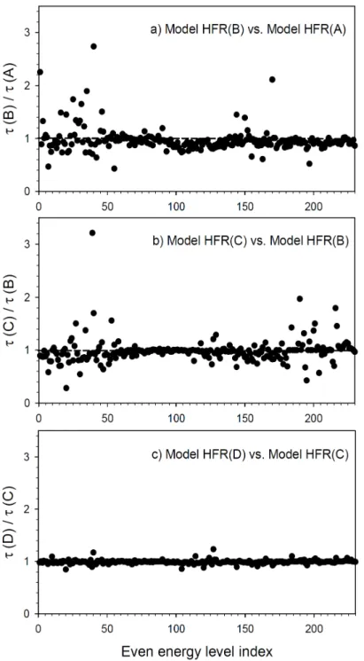
interacting configurations as the one considered in model HFR(C) was included with the additional permission that one electron could be excited on the 6f or the 7p subshell, giving rise to a total of 26 odd-parity and 25 even-parity configurations. Using the four HFR models presented hereabove, we computed and compared the radiative lifetimes for the 250 lowest even-parity energy levels with τ-values smaller than 100 ns. These comparisons are summarized in Figure 1 showing the ratios τ(B)/τ(A), τ(C)/τ(B) and τ(D)/τ(C), respectively. When looking at Figure 1a, it is clear that the numerous missing odd-parity configurations in the HFR(A) model, similar to the one used by Ryabtsev et al. [13], make without doubt this latter model insufficient to provide a reliable set of transition probabilities, the mean deviation between the HFR(B) and HFR(A) lifetimes being found to be within about 30%, with notable discrepancies reaching a factor of 2–3 in some cases. Moreover, Figure 1b shows that the HFR(B) model does not either include enough configuration interaction to give a reasonable accuracy of the radiative lifetime calculations, the differences between the data computed with models HFR(C) and HFR(B) still reaching a factor of 1.5–2 in many cases. However, as shown in Figure 1c, the excitations of one electron to the 6f or 7p subshell included in model HFR(D) do not really change the results obtained in model HFR(C), the mean deviation between both sets of lifetimes not exceeding 2%. We can therefore conclude that the one single excitation from 4f, 5s and 5p to nl orbitals with nl = 5d, 5f, 6s, 6p, 6d and 7s, as considered in the configuration interaction expansions of model HFR(C), should form a good basis for computing the spectroscopic data in W VIII.

Furthermore, it is also interesting to estimate the influence of the double excitations on the radiative parameters. Indeed, for transitions of the type 4f14_5s2_5p5 _{– 4f}14_5s2_5p4_{5d and 4f}13_5s2_5p6 _–

4f13_5s2_5p5_{5d, the 5p}2 _{→ 5d}2 _{double excitation in the lower odd-parity state leads to an allowed}

transition to the upper even-parity state with an electric dipole matrix element which is equal in magnitude to that for the primary transition. In order to evaluate this effect on the decay rates, we extended the multiconfiguration expansion of model HFR(C) with the two additional odd-parity configurations 4f14_5s2_5p3_5d2 _{and 4f}13_5s2_5p4_5d2_{, giving rise to model HFR(E). Finally, as similar}

speculations can be made for the double excitation 4f2 _{→ 5d}2 _{in the case of the 4f}14_5s2_5p5 _–

4f13_5s2_5p5_{5d and 4f}13_5s2_5p6 _{– 4f}12_5s2_5p6_{5d transitions and for the double excitation 5p}2 _{→ 6s}2 _{in the}

case of the 4f14_5s2_5p5 _{– 4f}14_5s2_5p4_{6s and 4f}13_5s2_5p6 _{– 4f}13_5s2_5p5_{6s transitions, the odd-parity}

configurations 4f12_5s2_5p5_5d2 _{and 4f}11_5s2_5p6_5d2 _{were added to model HFR(E) to give model HFR(F),}

while 4f14_5s2_5p3_6s2 _{and 4f}13_5s2_5p4_6s2 _{were added to model HFR(F) to give model HFR(G). The}

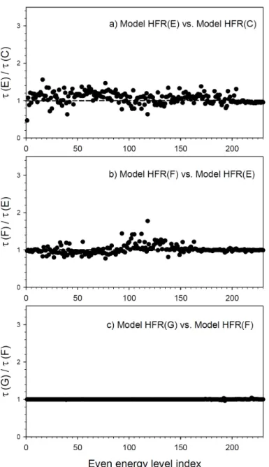
radiative lifetimes calculated with these latter models are compared to those obtained with HFR(C) in Figure 2. As observed in this figure, if the 5p2 _{→ 6s}2_{, considered in model HFR(G) do not change}

the final results (see Figure 2c), it is not the same for the 5p2 _{→ 5d}2 _{and 4f}2 _{→ 5d}2 _excitations,

respectively included in models HFR(E) and HFR(F), which both lead to non negligible changes in the computed radiative lifetimes by about 20% (see Figures 2a,2b). This is nevertheless not very surprising since this kind of effect was already highlighted by Quinet and Hansen [19] who

pointed out the influence of 3p2 _{→ 3d}2 _{core excitation on the 3p}6_3dN _{– 3p}5_3dN+1 _{transition rates in}

iron group elements.

Figure 1. Comparison between radiative lifetimes obtained in the present work using different HFR models for short-lived even-parity energy levels (τ < 100 ns) in W VIII. In each panel, the y-axis gives the ratio of τ -values computed with two successive models including only single excitations (see text) while the x-axis corresponds to the level indexes, assigned according to the order of increasing energies.

Figure 2. Comparison between radiative lifetimes obtained in the present work using different HFR models for short-lived even-parity energy levels (τ < 100 ns) in W VIII. In each panel, the y-axis gives the ratio of τ-values computed with two successive models including both single and double excitations (see text) while the x-axis corresponds to the level indexes, assigned according to the order of increasing energies.

4. Radiative Parameter Calculations

Further to the detailed discussion presented in the previous section, HFR(F) was chosen as the final model to compute the radiative parameters in W VIII. To summarize, the following configurations were explicitly included in the calculations: 4f13_5s2_5p6 _{+ 4f}14_5s2_5p5 _{+ 4f}14_5s2_5p4_{(5f + 6p) +}

4f14_5s5p5_{(5d + 6s + 6d + 7s) + 4f}13_5s2_5p5_{(5f + 6p) + 4f}13_5s5p6_{(5d + 6s + 6d + 7s) + 4f}14_5p6_{(5f + 6p) +}

4f12_5s2_5p6_{(5f + 6p) + 4f}14_5s2_5p3_5d2 _{+ 4f}13_5s2_5p4_5d2 _{+ 4f}12_5s2_5p5_5d2 _{+ 4f}11_5s2_5p6_5d2 _{(odd parity) and}

4f14_5s5p6 _{+ 4f}14_5s2_5p4_{(5d + 6s + 6d + 7s) + 4f}14_5s5p5_{(5f + 6p) + 4f}13_5s2_5p5_{(5d + 6s + 6d + 7s) +}

model was then combined with a semi-empirical adjustment of the radial energy parameters in order to minimize the discrepancies between calculated and available experimental energy levels. The strategy followed in the fitting process was exactly the same as the one developed by Ryabtsev et al. [13] to the extent that, starting with the numerical values given in their paper, the same parameters were adjusted with the same constraints as those used by these latter authors. This allowed us simply to adapt and optimize the final radial parameters to our physical model including a much larger number of interacting configurations than the model used in [13].

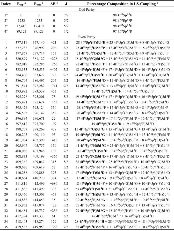
The numerical values of the radial parameters adopted in our work are reported in Table 1 while the calculated energy levels are compared to the experimental data in Table 2. For the 98 even-parity levels, the standard deviation of the fit was found to be equal to 438 cm−1 _{which is comparable to the}

value of 443 cm−1 _{obtained by Ryabtsev et al. [13]. When looking at the table, it appears that the}

ordering of experimental and calculated energy levels can be different in a few cases. This is simply due to the fact that some experimental level values are close to each other, with a difference of the same order of magnitude as the standard deviation mentioned above. However, in any case, the ordering of the calculated energies always corresponds to the observed one within a J-matrix. Table 2 also lists the first three LS-components for each level. We can note that, as expected, most of the even-parity states are very strongly mixed and, as already pointed out by Ryabtsev et al., the jj-coupling scheme given by these authors appears a bit more appropriate than the LS one, with average eigenvector purities of 45% and 32%, respectively. It is also worth mentioning that, if LS purities of 100% were reported by Ryabtsev et al., for the four levels belonging to the 4f13_5s2_5p6 _{and 4f}14_5s2_5p5 _{odd-parity configurations,}

it is no more the case in our extended configuration interaction model which gives slightly reduced purities of 97%–98% for those levels. In spite of their very strong mixing, the first LS-component of each level is given in boldface in Table 2.

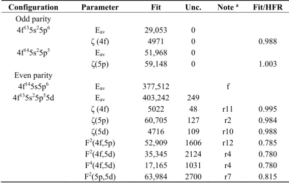
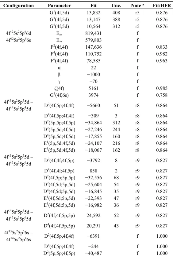
Table 1. Numerical values (in cm−1_{) of the radial energy parameters adopted in the}

Hartree-Fock (HFR) calculations.

Configuration Parameter Fit Unc. Note a _Fit/HFR

Odd parity 4f13_5s2_5p6 _E av 29,053 0 ζ (4f) 4971 0 0.988 4f14_5s2_5p5 _E av 51,968 0 ζ(5p) 59,148 0 1.003 Even parity 4f14_5s5p6 _E av 377,512 f 4f13_5s2_5p5_{5d E} av 403,242 249 ζ (4f) 5022 48 r11 0.995 ζ(5p) 60,705 127 r2 0.984 ζ(5d) 4716 109 r10 0.988 F2_{(4f,5p) 52,909 1606 r12 0.785} F2_{(4f,5d) 35,345 2124 r4 0.780} F4_{(4f,5d) 17,165 1031 r4 0.780} F2_{(5p,5d) 63,984 2700 r7 0.815}

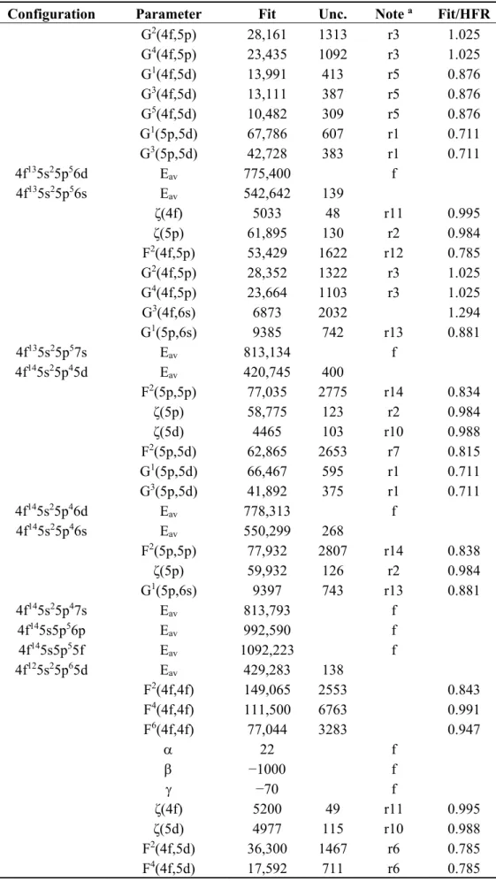
Table 1. Cont.

Configuration Parameter Fit Unc. Note a _Fit/HFR

G2_{(4f,5p) 28,161 1313 r3 1.025} G4_{(4f,5p) 23,435 1092 r3 1.025} G1_{(4f,5d) 13,991 413 r5 0.876} G3_{(4f,5d) 13,111 387 r5 0.876} G5_{(4f,5d) 10,482 309 r5 0.876} G1_{(5p,5d) 67,786 607 r1 0.711} G3_{(5p,5d) 42,728 383 r1 0.711} 4f13_5s2_5p5_{6d E} av 775,400 f 4f13_5s2_5p5_{6s E} av 542,642 139 ζ(4f) 5033 48 r11 0.995 ζ(5p) 61,895 130 r2 0.984 F2_{(4f,5p) 53,429 1622 r12 0.785} G2_{(4f,5p) 28,352 1322 r3 1.025} G4_{(4f,5p) 23,664 1103 r3 1.025} G3_{(4f,6s) 6873 2032 1.294} G1_{(5p,6s) 9385 742 r13 0.881} 4f13_5s2_5p5_{7s E} av 813,134 f 4f14_5s2_5p4_{5d E} av 420,745 400 F2_{(5p,5p) 77,035 2775 r14 0.834} ζ(5p) 58,775 123 r2 0.984 ζ(5d) 4465 103 r10 0.988 F2_{(5p,5d) 62,865 2653 r7 0.815} G1_{(5p,5d) 66,467 595 r1 0.711} G3_{(5p,5d) 41,892 375 r1 0.711} 4f14_5s2_5p4_{6d E} av 778,313 f 4f14_5s2_5p4_{6s E} av 550,299 268 F2_{(5p,5p) 77,932 2807 r14 0.838} ζ(5p) 59,932 126 r2 0.984 G1_{(5p,6s) 9397 743 r13 0.881} 4f14_5s2_5p4_{7s E} av 813,793 f 4f14_5s5p5_{6p E} av 992,590 f 4f14_5s5p5_{5f E} av 1092,223 f 4f12_5s2_5p6_{5d E} av 429,283 138 F2_{(4f,4f) 149,065 2553 0.843} F4_{(4f,4f) 111,500 6763 0.991} F6_{(4f,4f) 77,044 3283 0.947}  22 f  −1000 f  −70 f ζ(4f) 5200 49 r11 0.995 ζ(5d) 4977 115 r10 0.988 F2_{(4f,5d) 36,300 1467 r6 0.785} F4_{(4f,5d) 17,592 711 r6 0.785}

Table 1. Cont.

Configuration Parameter Fit Unc. Note a _Fit/HFR

G1_{(4f,5d) 13,832 408 r5 0.876} G3_{(4f,5d) 13,147 388 r5 0.876} G5_{(4f,5d) 10,564 312 r5 0.876} 4f12_5s2_5p6_{6d E} av 819,431 f 4f12_5s2_5p6_{6s E} av 579,803 f F2_{(4f,4f) 147,636 f 0.833} F4_{(4f,4f) 110,752 f 0.982} F6_{(4f,4f) 78,585 f 0.963} α 22 f  −1000 f  −70 f ζ(4f) 5161 f 0.985 G3_{(4f,6s) 3974 f 0.758} 4f13_5s2_5p5_{5d –} 4f14_5s2_5p4_5d D2(4f,5p;4f,4f) −5660 51 r8 0.864 D4_{(4f,5p;4f,4f) −309 3 r8 0.864} D2_{(5p,5p;4f,5p) −34,864 312 r8 0.864} D2_{(5p,5d;4f,5d) −27,246 244 r8 0.864} D4_{(5p,5d;4f,5d) −17,855 160 r8 0.864} E1_{(5p,5d;4f,5d) −24,107 216 r8 0.864} E3_{(5p,5d;4f,5d) −18,067 162 r8 0.864} 4f13_5s2_5p5_{5d –} 4f12_5s2_5p6_5d D2(4f,4f;4f,5p) −3792 8 r9 0.827 D4_{(4f,4f;4f,5p) 858 2 r9 0.827} D2_{(4f,5p;5p,5p) −32,556 68 r9 0.827} D2_{(4f,5d;5p,5d) −25,604 54 r9 0.827} D4_{(4f,5d;5p,5d) −16,845 35 r9 0.827} E1_{(4f,5d;5p,5d) −22,393 47 r9 0.827} E3_{(4f,5d;5p,5d) −16,982 36 r9 0.827} 4f14_5s2_5p4_{5d –} 4f12_5s2_5p6_5d D2(4f,4f;5p,5p) 24,592 52 r9 0.827 D4_{(4f,4f;5p,5p) 20,291 43 r9 0.827} 4f13_5s2_5p5_{6s –} 4f14_5s2_5p4_6s D2(4f,5p,4f,4f) −6391 f 1.000 D4_{(4f,5p;4f,4f) −244 f 1.000} D2_{(5p,5p;4f,5p) −40,487 f 1.000}

Table 2. Comparison between the energy levels computed in the present work and the experimentally known values available in seven times ionized tungsten (W VIII). Energies are given in cm−1_.

Index Eexpa Ecalcb ΔE c J Percentage Composition in LS-Coupling d Odd Parity 1° 0 0 0 7/2 98 4f13_5p62_F 2° 1233 1233 0 3/2 98 4f14_5p52_P 3° 17,410 17,410 0 5/2 98 4f13_5p62_F 4° 89,123 89,123 0 1/2 97 4f14_5p52_P Even Parity 1 377,119 377,140 −21 9/2 28 4f13_5p5₍3_F)5d 2_{H + 23 4f}13_5p5₍1_D)5d 2_{G + 8 4f}13_5p5₍3_F)5d 2_G 2 377,288 376,992 296 3/2 25 4f13_5p5₍1_D)5d 2_{P + 18 4f}13_5p5₍3_D)5d 4_{F + 15 4f}13_5p5₍3_D)5d 4_P 3 377,867 377,714 153 5/2 21 4f13_5p5₍3_D)5d 4_{F + 12 4f}14_5p4₍1_S)5d 2_{D + 9 4f}13_5p5₍3_F)5d 2_F 4 380,899 381,127 −228 9/2 18 4f13_5p5₍1_G)5d 2_{G + 18 4f}13_5p5₍3_G)5d 2_{G + 14 4f}13_5p5₍3_F)5d 2_G 5 382,019 382,285 −266 7/2 22 4f13_5p5₍1_D)5d 2_{F + 15 4f}13_5p5₍3_D)5d 2_{G + 13 4f}13_5p5₍3_F)5d 2_F 6 383,133 383,535 −402 5/2 18 4f13_5p5₍3_D)5d 2_{F + 17 4f}13_5p5₍1_D)5d 2_{D + 10 4f}14_5p4₍1_S)5d 2_D 7 384,400 383,622 778 9/2 24 4f13_5p5₍1_G)5d 2_{H + 20 4f}13_5p5₍3_G)5d 4_{H + 11 4f}13_5p5₍3_D)5d 4_G 8 386,704 386,497 207 5/2 16 4f13_5p5₍3_F)5d 2_{D + 11 4f}13_5p5₍3_G)5d 4_{D + 9 4f}13_5p5₍3_F)5d 4_P 9 391,541 392,282 −741 9/2 14 4f13_5p5₍1_D)5d 2_{G + 13 4f}12_5p6₍3_H)5d 2_{G + 5 4f}13_5p5₍3_G)5d 2_H 10 393,992 393,539 453 7/2 18 4f12_5p6₍3_H)5d 2_{F + 14 4f}13_5p5₍3_G)5d 2_F 11 395,276 395,201 75 5/2 19 4f13_5p5₍3_D)5d 2_{F + 17 4f}13_5p5₍3_D)5d 4_{D + 16 4f}13_5p5₍3_D)5d 4_F 12 395,471 395,624 −153 7/2 14 4f12_5p6₍3_F)5d 4_{F + 11 4f}13_5p5₍3_F)5d 2_{G + 8 4f}12_5p6₍3_F)5d 4_D 13 395,474 395,124 350 1/2 38 4f14_5p4₍3_P)5d 4_{P + 17 4f}13_5p5₍3_D)5d 2_{S + 8 4f}14_5p4₍3_P)5d 2_P 14 396,505 396,147 358 7/2 20 4f13_5p5₍3_D)5d 4_{F + 14 4f}13_5p5₍3_F)5d 2_{G + 8 4f}13_5p5₍3_D)5d 2_F 15 396,894 396,671 22 3/2 17 4f13_5p5₍3_F)5d 2_{P + 17 4f}14_5p4₍3_P)5d 4_{P + 16 4f}14_5p4₍3_P)5d 4_F 16 397,612 397,709 −97 5/2 19 4f12_5p6₍1_G)5d 2_{D + 19 4f}12_5p6₍3_F)5d 4_D 17 398,707 398,269 438 9/2 15 4f13_5p5₍1_G)5d 2_{G + 15 4f}13_5p5₍3_G)5d 4_{G + 13 4f}13_5p5₍1_G)5d 2_H 18 400,203 400,110 93 9/2 19 4f12_5p6₍3_F)5d 4_{G + 14 4f}12_5p6₍1_G)5d 2_{H + 13 4f}12_5p6₍3_F)5d 4_F 19 401,984 402,399 −415 5/2 20 4f14_5p4₍3_P)5d 4_{F + 17 4f}13_5p5₍3_G)5d 2_{D + 8 4f}14_5p4₍1_D)5d 2_F 20 405,907 405,757 150 9/2 41 4f12_5p6₍3_H)5d 4_{G + 25 4f}12_5p6₍3_H)5d 4_{H + 8 4f}12_5p6₍3_H)5d 4_F 21 408,086 407,948 138 7/2 42 4f12_5p6₍3_H)5d 2_{F + 7 4f}12_5p6₍3_F)5d 2_{F + 7 4f}12_5p6₍1_G)5d 2_F 22 408,833 409,199 −366 3/2 21 4f12_5p6₍1_G)5d 2_{D + 17 4f}12_5p6₍1_D)5d 2_{D + 8 4f}12_5p6₍3_F)5d 2_D 23 409,362 409,047 315 5/2 38 4f12_5p6₍3_H)5d 4_{F + 25 4f}12_5p6₍3_F)5d 4_{F + 10 4f}12_5p6₍1_G)5d 2_D 24 409,676 409,619 57 5/2 18 4f12_5p6₍3_F)5d 4_{P + 16 4f}12_5p6₍3_F)5d 4_{G + 10 4f}12_5p6₍3_H)5d 2_F 25 410,258 409,885 373 3/2 17 4f12_5p6₍3_F)5d 2_{D + 13 4f}13_5p5₍3_G)5d 4_{F + 12 4f}13_5p5₍1_G)5d 2_D 26 410,654 410,270 384 7/2 13 4f12_5p6₍3_F)5d 4_{G + 9 4f}12_5p6₍3_H)5d 2_{G + 8 4f}13_5p5₍3_D)5d 2_G 27 411,819 412,499 −680 5/2 18 4f12_5p6₍3_H)5d 2_{F + 10 4f}13_5p5₍3_G)5d 4_{G + 10 4f}12_5p6₍3_F)5d 4_G 28 411,832 411,499 333 7/2 23 4f12_5p6₍3_F)5d 4_{D + 21 4f}12_5p6₍3_F)5d 4_{H + 14 4f}12_5p6₍1_G)5d 2_G 29 413,450 413,503 −53 9/2 28 4f12_5p6₍3_H)5d 2_{G + 13 4f}12_5p6₍3_F)5d 4_{H + 12 4f}12_5p6₍3_H)5d 4_I 30 414,888 414,853 35 7/2 39 4f12_5p6₍3_F)5d 4_{G + 11 4f}12_5p6₍3_F)5d 2_{F + 10 4f}12_5p6₍3_F)5d 4_H 31 415,852 415,874 −22 5/2 27 4f12_5p6₍3_F)5d 4_{G + 16 4f}12_5p6₍1_G)5d 2_{F + 13 4f}12_5p6₍3_F)5d 4_P 32 416,481 416,737 −256 9/2 29 4f12_5p6₍3_F)5d 2_{G + 18 4f}12_5p6₍3_H)5d 4_{I + 10 4f}12_5p6₍1_G)5d 2_G 33 417,394 417,333 61 3/2 42 4f12_5p6₍3_F)5d 2_{P + 16 4f}12_5p6₍1_G)5d 2_D 34 418,403 418,274 129 9/2 28 4f12_5p6₍3_F)5d 4_{H + 28 4f}12_5p6₍3_H)5d 2_{G + 18 4f}12_5p6₍3_H)5d 4_G 35 419,585 419,953 −368 7/2 35 4f12_5p6₍3_H)5d 4_{G + 11 4f}12_5p6₍3_F)5d 4_{F + 10 4f}12_5p6₍3_H)5d 4_F

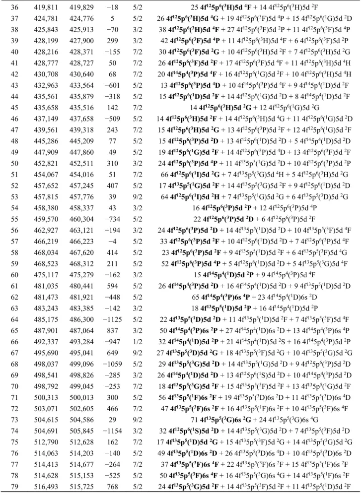
Table 2. Cont.

Index Eexpa Ecalcb ΔE c J Percentage Composition in LS-Coupling d 36 419,811 419,829 −18 5/2 25 4f12_5p6₍3_H)5d 4_{F + 14 4f}12_5p6₍3_H)5d 2_F 37 424,781 424,776 5 5/2 26 4f12_5p6₍3_H)5d 4_{G + 19 4f}12_5p6₍3_F)5d 4_{P + 15 4f}12_5p6₍1_G)5d 2_D 38 425,843 425,913 −70 3/2 38 4f12_5p6₍3_H)5d 4_{F + 27 4f}12_5p6₍3_F)5d 2_{P + 11 4f}12_5p6₍3_F)5d 4_P 39 428,199 427,900 299 3/2 42 4f12_5p6₍3_F)5d 4_{P + 11 4f}12_5p6₍3_H)5d 4_{F + 6 4f}12_5p6₍3_F)5d 2_P 40 428,216 428,371 −155 7/2 30 4f12_5p6₍3_F)5d 2_{G + 10 4f}12_5p6₍3_H)5d 2_{F + 7 4f}12_5p6₍3_H)5d 2_G 41 428,777 428,727 50 7/2 26 4f12_5p6₍3_F)5d 2_{F + 17 4f}12_5p6₍3_F)5d 4_{F + 11 4f}12_5p6₍3_H)5d 4_H 42 430,708 430,640 68 7/2 20 4f14_5p4₍3_P)5d 4_{F + 16 4f}12_5p6₍1_G)5d 2_{F + 10 4f}12_5p6₍3_H)5d 4_H 43 432,963 433,564 −601 5/2 13 4f12_5p6₍3_P)5d 4_{D + 10 4f}14_5p4₍3_P)5d 4_{F + 9 4f}14_5p4₍1_D)5d 2_F 44 435,561 435,879 −318 5/2 15 4f12_5p6₍1_D)5d 2_{F + 14 4f}12_5p6₍1_G)5d 2_{D + 8 4f}14_5p4₍1_D)5d 2_F 45 435,658 435,516 142 7/2 14 4f12_5p6₍3_H)5d 2_{G + 12 4f}12_5p6₍1_G)5d 2_G 46 437,149 437,658 −509 5/2 14 4f12_5p6₍3_H)5d 2_{F + 14 4f}12_5p6₍3_H)5d 4_{G + 11 4f}12_5p6₍1_G)5d 2_D 47 439,561 439,318 243 7/2 15 4f12_5p6₍3_H)5d 2_{G + 13 4f}12_5p6₍3_P)5d 2_{F + 12 4f}12_5p6₍1_G)5d 2_F 48 445,286 445,209 77 5/2 15 4f12_5p6₍3_P)5d 2_{D + 13 4f}12_5p6₍1_D)5d 2_{D + 5 4f}14_5p4₍1_D)5d 2_D 49 447,909 447,860 49 5/2 19 4f12_5p6₍1_G)5d 2_{F + 14 4f}12_5p6₍3_P)5d 4_{D + 13 4f}12_5p6₍3_F)5d 2_F 50 452,821 452,511 310 3/2 24 4f12_5p6₍3_P)5d 4_{P + 11 4f}13_5p5₍1_G)5d 2_{D + 10 4f}12_5p6₍3_P)5d 2_P 51 454,067 454,016 51 7/2 66 4f12_5p6₍1_I)5d 2_{G + 7 4f}13_5p5₍3_G)5d 4_{H + 5 4f}12_5p6₍3_H)5d 2_G 52 457,652 457,245 407 5/2 17 4f13_5p5₍1_G)5d 2_{F + 14 4f}13_5p5₍3_G)5d 2_{F + 9 4f}12_5p6₍1_D)5d 2_D 53 457,815 457,776 39 9/2 64 4f12_5p6₍1_I)5d 2_{H + 7 4f}13_5p5₍1_G)5d 2_{G + 6 4f}13_5p5₍3_D)5d 2_G 54 458,380 458,337 43 3/2 16 4f12_5p6₍3_P)5d 2_{P + 12 4f}12_5p6₍3_P)5d 4_P 55 459,570 460,304 −734 5/2 22 4f12_5p6₍3_P)5d 2_{D + 6 4f}12_5p6₍3_P)5d 2_F 56 462,927 463,121 −194 3/2 24 4f12_5p6₍3_P)5d 2_{D + 14 4f}13_5p5₍1_D)5d 2_{D + 10 4f}13_5p5₍3_F)5d 4_F 57 466,219 466,223 −4 5/2 33 4f12_5p6₍3_P)5d 2_{F + 10 4f}12_5p6₍1_D)5d 2_{D + 7 4f}12_5p6₍3_P)5d 4_F 58 468,034 467,620 414 5/2 23 4f12_5p6₍3_P)5d 2_{F + 9 4f}13_5p5₍1_D)5d 2_{F + 6 4f}13_5p5₍3_F)5d 4_G 59 468,523 468,312 211 5/2 52 4f12_5p6₍3_P)5d 4_{P + 5 4f}12_5p6₍1_D)5d 2_{D + 5 4f}13_5p5₍3_G)5d 4_F 60 475,117 475,279 −162 3/2 15 4f14_5p4₍1_D)5d 2_{P + 9 4f}14_5p4₍3_P)5d 4_F 61 481,035 480,441 594 5/2 26 4f14_5p4₍3_P)5d 2_{D + 16 4f}14_5p4₍1_D)5d 2_{D + 9 4f}13_5p5₍1_D)5d 2_D 62 481,473 481,921 −448 5/2 65 4f14_5p4₍3_P)6s 4_{P + 23 4f}14_5p4₍1_D)6s 2_D 63 483,243 483,385 −142 3/2 18 4f13_5p5₍1_D)5d 2_{P + 16 4f}14_5p4₍1_D)5d 2_P 64 485,175 486,300 −1125 5/2 22 4f13_5p5₍1_D)5d 2_{D + 11 4f}13_5p5₍1_D)5d 2_{F + 7 4f}13_5p5₍3_F)5d 4_F 65 487,901 487,064 837 3/2 50 4f14_5p4₍3_P)6s 2_{P + 27 4f}14_5p4₍1_D)6s 2_{D + 13 4f}14_5p4₍3_P)6s 4_P 66 492,337 493,284 −947 1/2 32 4f14_5p4₍1_D)5d 2_{P + 21 4f}14_5p4₍1_D)5d 2_{S + 16 4f}14_5p4₍3_P)5d 2_P 67 495,690 495,041 649 9/2 27 4f13_5p5₍3_D)5d 2_{G + 18 4f}13_5p5₍3_F)5d 2_{G + 10 4f}13_5p5₍3_G)5d 2_G 68 498,037 499,096 −1059 5/2 29 4f13_5p5₍3_G)5d 2_{D + 14 4f}13_5p5₍1_G)5d 2_{D + 9 4f}12_5p6₍3_P)5d 2_D 69 498,541 498,826 −285 3/2 26 4f14_5p4₍1_D)5d 2_{D + 13 4f}12_5p6₍1_S)5d 2_{D + 10 4f}14_5p4₍3_P)5d 2_D 70 498,792 499,045 −253 7/2 18 4f13_5p5₍3_G)5d 2_{F + 15 4f}13_5p5₍3_F)5d 2_{F + 13 4f}13_5p5₍1_G)5d 2_F 71 500,313 500,013 300 5/2 56 4f13_5p5₍1_F)6s 2_{F + 19 4f}13_5p5₍3_D)6s 2_{D + 11 4f}13_5p5₍3_D)6s 4_D 72 503,071 502,605 466 7/2 47 4f13_5p5₍3_F)6s 2_{F + 16 4f}13_5p5₍1_F)6s 2_{F + 10 4f}13_5p5₍3_F)6s 4_F 73 504,615 504,586 29 9/2 71 4f13_5p5₍3_G)6s 2_{G + 24 4f}13_5p5₍3_G)6s 4_G 74 504,691 505,845 −1154 3/2 32 4f12_5p6₍1_S)5d 2_{D + 14 4f}13_5p5₍3_G)5d 2_{D + 7 4f}13_5p5₍3_F)5d 2_D 75 512,790 512,628 162 7/2 17 4f13_5p5₍1_D)5d 2_{G + 15 4f}13_5p5₍3_F)5d 2_{G + 14 4f}13_5p5₍3_G)5d 2_G 76 514,063 514,203 −140 5/2 49 4f13_5p5₍1_D)6s 2_{D + 26 4f}13_5p5₍3_D)6s 4_{D + 10 4f}13_5p5₍3_D)6s 2_D 77 514,413 514,677 −264 7/2 37 4f13_5p5₍3_F)6s 4_{F + 22 4f}13_5p5₍3_F)6s 2_{F + 15 4f}13_5p5₍1_F)6s 2_F 78 514,628 515,153 −525 5/2 50 4f13_5p5₍3_F)6s 4_{F + 16 4f}13_5p5₍3_G)6s 4_{G + 14 4f}13_5p5₍1_F)6s 2_F 79 516,493 515,725 768 5/2 24 4f13_5p5₍3_G)5d 2_{F + 14 4f}13_5p5₍3_F)5d 2_{F + 11 4f}13_5p5₍1_D)5d 2_F

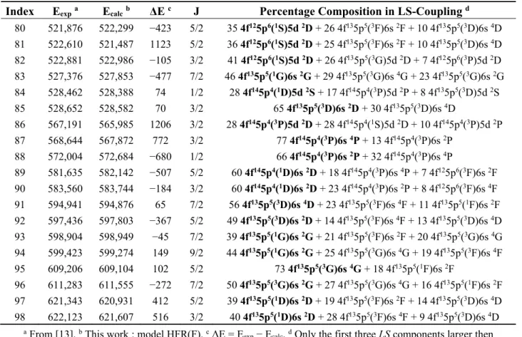
Table 2. Cont.

Index Eexpa Ecalcb ΔE c J Percentage Composition in LS-Coupling d 80 521,876 522,299 −423 5/2 35 4f12_5p6₍1_S)5d 2_{D + 26 4f}13_5p5₍3_F)6s 2_{F + 10 4f}13_5p5₍3_D)6s 4_D 81 522,610 521,487 1123 5/2 36 4f12_5p6₍1_S)5d 2_{D + 25 4f}13_5p5₍3_F)6s 2_{F + 10 4f}13_5p5₍3_D)6s 4_D 82 522,881 522,986 −105 3/2 41 4f12_5p6₍1_S)5d 2_{D + 26 4f}13_5p5₍3_G)5d 2_{D + 7 4f}12_5p6₍3_P)5d 2_D 83 527,376 527,853 −477 7/2 46 4f13_5p5₍1_G)6s 2_{G + 29 4f}13_5p5₍3_G)6s 4_{G + 23 4f}13_5p5₍3_G)6s 2_G 84 528,462 528,388 74 1/2 28 4f14_5p4₍1_D)5d 2_{S + 17 4f}14_5p4₍3_P)5d 2_{P + 8 4f}13_5p5₍3_D)5d 2_S 85 528,652 528,582 70 3/2 65 4f13_5p5₍3_D)6s 2_{D + 30 4f}13_5p5₍3_D)6s 4_D 86 567,191 565,985 1206 3/2 28 4f14_5p4₍3_P)5d 2_{D + 28 4f}14_5p4₍1_S)5d 2_{D + 10 4f}14_5p4₍3_P)5d 2_P 87 568,644 567,872 772 3/2 77 4f14_5p4₍3_P)6s 4_{P + 13 4f}14_5p4₍3_P)6s 2_P 88 572,004 572,684 −680 1/2 66 4f14_5p4₍3_P)6s 2_{P + 32 4f}14_5p4₍3_P)6s 4_P 89 581,635 582,142 −507 5/2 60 4f14_5p4₍1_D)6s 2_{D + 18 4f}14_5p4₍3_P)6s 4_{P + 7 4f}12_5p6₍3_F)6s 2_F 90 583,560 583,744 −184 3/2 60 4f14_5p4₍1_D)6s 2_{D + 23 4f}14_5p4₍3_P)6s 2_{P + 8 4f}12_5p6₍3_F)6s 4_F 91 594,941 594,876 65 7/2 56 4f13_5p5₍3_D)6s 4_{D + 23 4f}13_5p5₍3_F)6s 4_{F + 11 4f}13_5p5₍1_F)6s 2_F 92 597,436 597,803 −367 5/2 49 4f13_5p5₍3_D)6s 2_{D + 14 4f}13_5p5₍3_F)6s 4_{F + 13 4f}13_5p5₍3_D)6s 4_D 93 598,904 598,949 −45 7/2 39 4f13_5p5₍1_G)6s 2_{G + 21 4f}13_5p5₍3_F)6s 2_{F + 20 4f}13_5p5₍3_G)6s 4_G 94 599,423 599,274 149 9/2 44 4f13_5p5₍1_G)6s 2_{G + 25 4f}13_5p5₍3_G)6s 4_{G + 19 4f}13_5p5₍3_F)6s 4_F 95 609,206 609,104 102 5/2 73 4f13_5p5₍3_G)6s 4_{G + 18 4f}13_5p5₍1_F)6s 2_F 96 611,283 611,555 −272 7/2 50 4f13_5p5₍3_G)6s 2_{G + 27 4f}13_5p5₍3_G)6s 4_{G + 16 4f}13_5p5₍1_F)6s 2_F 97 621,343 620,931 412 5/2 39 4f13_5p5₍1_D)6s 2_{D + 19 4f}13_5p5₍3_F)6s 2_{F + 14 4f}13_5p5₍3_D)6s 4_D 98 622,123 621,607 516 3/2 40 4f13_5p5₍1_D)6s 2_{D + 28 4f}13_5p5₍3_F)6s 4_{F + 9 4f}13_5p5₍3_D)6s 4_D a _{From [13].} b _{This work : model HFR(F).} c _{ΔE = E}

exp − Ecalc. d Only the first three LS components larger then

5% are given.

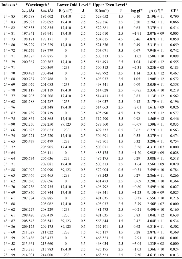
The calculated oscillator strengths (log gf) and transition probabilities (gA) obtained in the present work are given in Table 3 for all the W VIII spectral lines with log gf-values greater than −4. These parameters are only given in the length form, the HFR code of Cowan not allowing the calculation of radiative decay rates in the velocity form. Observed wavelengths (ëexp) taken from the

work of Ryabtsev et al. [13] are also given in the same table together with the 'Ritz' wavelengths (λRitz)

deduced from the experimental energy levels identified by the same authors. When looking in detail at the table, one can see that forty listed lines were not observed in [13]. If most of those lines are characterized by rather weak transition probabilities, three of them appear to be strong enough, i.e., with gA-values greater than 1010 _s−1_{, to be experimentally observed, according to our calculations.}

These are located at λ = 191.700 Å (gA = 1.46 × 1010 _s−1_{), λ = 229.402 Å (gA = 1.16 × 10}10 _s−1_{) and λ}

= 244.249 Å (gA = 1.33 × 1011 _s−1_{) and correspond respectively to transitions from the lower odd level}

at 1233 cm−1 _{(J = 3/2), to the upper even level at 522,881 cm}−1 _{(J = 3/2), from the lower odd level at}

1233 cm−1 _{(J = 3/2) to the upper even level at 437,149 cm}−1 _{(J = 5/2), and from the lower odd level at}

Table 3. Oscillator strengths and transition probabilities in W VIII (log gf > −4). A table entry 6.81E + 08 means 6.81×108_.

Indexes a _Wavelength b _{Lower Odd Level} c _{Upper Even Level} c

λexp (Å) λRitz (Å) E (cm−1) J E (cm−1) J log gf d gA (s-1) d CF e

1° − 97 160.940 160.942 0 3.5 621,343 2.5 −2.58 6.81E + 08 0.003 2° − 98 161.057 161.059 1233 1.5 622,123 1.5 −2.41 1.01E + 09 0.045 2° − 97 161.260 161.262 1233 1.5 621,343 2.5 −1.26 1.40E + 10 0.333 1° − 96 163.596 163.590 0 3.5 611,283 3.5 −2.30 1.24E + 09 0.007 1° − 95 164.143 164.148 0 3.5 609,206 2.5 −2.78 4.15E + 08 0.014 2° − 95 164.479 164.481 1233 1.5 609,206 2.5 −3.29 1.27E + 08 0.226 3° − 98 165.369 165.368 17,410 2.5 622,123 1.5 −0.26 1.34E + 11 0.854 3° − 97 165.583 165.581 17,410 2.5 621,343 2.5 −0.42 9.25E + 10 0.609 1° − 94 166.827 166.827 0 3.5 599,423 4.5 0.15 3.39E + 11 0.872 1° − 93 166.971 166.972 0 3.5 598,904 3.5 −0.22 1.44E + 11 0.558 1° − 92 167.382 167.382 0 3.5 597,436 2.5 −0.04 2.16E + 11 0.721 1° − 91 168.084 168.084 0 3.5 594,941 3.5 −0.56 6.57E + 10 0.820 3° − 96 168.381 168.386 17,410 2.5 611,283 3.5 0.05 2.62E + 11 0.730 3° − 95 168.980 168.977 17,410 2.5 609,206 2.5 −0.59 6.03E + 10 0.778 2° − 90 171.727 171.725 1233 1.5 583,560 1.5 −0.80 3.56E + 10 0.131 1° − 89 171.929 0 3.5 581,635 2.5 −2.76 3.98E + 08 0.038 3° − 93 171.973 171.971 17,410 2.5 598,904 3.5 −1.70 4.48E + 09 0.013 2° − 89 172.295 172.294 1233 1.5 581,635 2.5 −0.19 1.46E + 11 0.641 3° − 91 173.151 17,410 2.5 594,941 3.5 −2.67 4.74E + 08 0.026 2° − 88 175.199 175.202 1233 1.5 572,004 0.5 −0.58 5.76E + 10 0.632 2° − 87 176.237 176.239 1233 1.5 568,644 1.5 −0.80 3.38E + 10 0.039 3° − 90 176.630 176.632 17,410 2.5 583,560 1.5 −1.27 1.15E + 10 0.701 2° − 86 176.694 176.692 1233 1.5 567,191 1.5 −0.75 3.77E + 10 0.030 3° − 89 177.232 177.234 17,410 2.5 581,635 2.5 −1.36 9.27E + 09 0.591 3° − 87 181.410 181.411 17,410 2.5 568,644 1.5 −1.07 1.74E + 10 0.134 3° − 86 181.888 181.891 17,410 2.5 567,191 1.5 −0.67 4.28E + 10 0.176 4° − 98 187.608 187.617 89,123 0.5 622,123 1.5 −1.50 5.93E + 09 0.256 2° − 85 189.603 1233 1.5 528,652 1.5 −2.44 6.70E + 08 0.083 1° − 83 189.616 189.618 0 3.5 527,376 3.5 −1.17 1.25E + 10 0.452 2° − 84 189.667 189.671 1233 1.5 528,462 0.5 −0.59 4.81E + 10 0.030 1° − 81 191.348 191.347 0 3.5 522,610 2.5 −0.67 3.89E + 10 0.082 1° − 80 191.617 191.616 0 3.5 521,876 2.5 −0.46 6.38E + 10 0.102 2° − 82 191.700 1233 1.5 522,881 1.5 −1.10 1.46E + 10 0.069 2° − 81 191.800 1233 1.5 522,610 2.5 −3.00 1.78E + 08 0.001 2° − 80 192.070 192.070 1233 1.5 521,876 2.5 −2.25 1.02E + 09 0.007 1° − 79 193.614 193.613 0 3.5 516,493 2.5 −0.96 1.95E + 10 0.029 2° − 79 194.077 194.077 1233 1.5 516,493 2.5 −1.37 7.51E + 09 0.095 1° − 78 194.315 194.315 0 3.5 514,628 2.5 −2.94 2.05E + 08 0.011 1° − 77 194.397 194.396 0 3.5 514,413 3.5 −0.59 4.58E + 10 0.047 1° − 76 194.527 194.529 0 3.5 514,063 2.5 0.09 2.19E + 11 0.840 2° − 76 194.998 194.996 1233 1.5 514,063 2.5 −1.46 6.02E + 09 0.403 1° − 75 195.021 195.012 0 3.5 512,790 3.5 −1.64 4.01E + 09 0.003

Table 3. Cont.

Indexes a _Wavelength b _{Lower Odd Level} c _{Upper Even Level} c

λexp (Å) λRitz (Å) E (cm−1) J E (cm−1) J log gf d gA (s-1) d CF e

3° − 85 195.598 195.602 17,410 2.5 528,652 1.5 0.10 2.19E + 11 0.790 3° − 83 196.093 196.092 17,410 2.5 527,376 3.5 0.20 2.76E + 11 0.866 3° − 82 197.835 197.835 17,410 2.5 522,881 1.5 0.63 7.37E + 11 0.514 3° − 81 197.941 197.941 17,410 2.5 522,610 2.5 −1.91 2.07E + 09 0.005 1° − 73 198.171 198.171 0 3.5 504,615 4.5 0.46 4.87E + 11 0.850 3° − 80 198.229 198.229 17,410 2.5 521,876 2.5 0.49 5.31E + 11 0.659 1° − 72 198.779 198.779 0 3.5 503,071 3.5 0.67 7.94E + 11 0.742 1° − 71 199.875 199.875 0 3.5 500,313 2.5 −1.02 1.58E + 10 0.098 3° − 79 200.367 200.367 17,410 2.5 516,493 2.5 1.04 1.82E + 12 0.555 2° − 71 200.369 1233 1.5 500,313 2.5 −2.31 8.23E + 08 0.183 1° − 70 200.483 200.484 0 3.5 498,792 3.5 1.14 2.31E + 12 0.467 1° − 68 200.787 200.788 0 3.5 498,037 2.5 1.05 1.90E + 12 0.572 2° − 69 201.079 201.083 1233 1.5 498,541 1.5 0.09 2.05E + 11 0.358 3° − 78 201.119 201.119 17,410 2.5 514,628 2.5 −0.85 2.33E + 10 0.219 3° − 77 201.205 201.206 17,410 2.5 514,413 3.5 0.83 1.13E + 12 0.562 2° − 68 201.288 201.287 1233 1.5 498,037 2.5 0.12 2.17E + 11 0.196 3° − 76 201.348 17,410 2.5 514,063 2.5 −2.01 1.61E + 09 0.026 1° − 67 201.739 201.739 0 3.5 495,690 4.5 1.29 3.22E + 12 0.577 3° − 75 201.864 201.865 17,410 2.5 512,790 3.5 0.98 1.56E + 12 0.446 4° − 90 202.250 202.250 89,123 0.5 583,560 1.5 −0.07 1.39E + 11 0.835 2° − 66 203.623 203.623 1233 1.5 492,337 0.5 0.62 6.72E + 11 0.563 3° − 74 205.221 205.220 17,410 2.5 504,691 1.5 0.53 5.37E + 11 0.474 2° − 65 205.479 205.479 1233 1.5 487,901 1.5 0.32 3.29E + 11 0.754 3° − 72 205.905 17,410 2.5 503,071 3.5 −3.56 4.31E + 07 0.000 1° − 64 206.111 0 3.5 485,175 2.5 −1.20 9.98E + 09 0.028 2° − 64 206.634 206.636 1233 1.5 485,175 2.5 0.29 3.08E + 11 0.518 3° − 71 207.081 17,410 2.5 500,313 2.5 −1.64 3.56E + 09 0.020 4° − 88 207.092 207.090 89,123 0.5 572,004 0.5 −0.31 7.59E + 10 0.784 2° − 63 207.466 207.465 1233 1.5 483,243 1.5 0.27 2.86E + 11 0.266 1° − 62 207.690 207.696 0 3.5 481,473 2.5 −0.69 3.20E + 10 0.364 3° − 70 207.736 207.735 17,410 2.5 498,792 3.5 −0.80 2.49E + 10 0.027 3° − 69 207.850 207.844 17,410 2.5 498,541 1.5 −1.23 9.15E + 09 0.025 1° − 61 207.884 207.885 0 3.5 481,035 2.5 −0.37 6.55E + 10 0.216 3° − 68 208.062 17,410 2.5 498,037 2.5 −3.79 2.56E + 07 0.000 2° − 62 208.227 208.229 1233 1.5 481,473 2.5 −0.21 9.49E + 10 0.160 2° − 61 208.420 208.419 1233 1.5 481,035 2.5 0.83 1.04E + 12 0.638 4° − 87 208.543 208.541 89,123 0.5 568,644 1.5 0.42 4.04E + 11 0.534 4° − 86 209.175 209.175 89,123 0.5 567,191 1.5 0.62 6.31E + 11 0.502 2° − 60 211.027 211.022 1233 1.5 475,117 1.5 0.28 2.87E + 11 0.369 1° − 59 213.436 213.437 0 3.5 468,523 2.5 −2.91 1.81E + 08 0.001 1° − 58 213.661 213.660 0 3.5 468,034 2.5 −3.04 1.33E + 08 0.000 3° − 64 213.785 213.783 17,410 2.5 485,175 2.5 −1.03 1.36E + 10 0.024 2° − 59 214.001 214.000 1233 1.5 468,523 2.5 −2.50 4.61E + 09 0.013

Table 3. Cont.

Indexes a _Wavelength b _{Lower Odd Level} c _{Upper Even Level} c

λexp (Å) λRitz (Å) E (cm−1) J E (cm−1) J log gf d gA (s-1) d CF e

2° − 58 214.229 214.224 1233 1.5 468,034 2.5 −0.09 1.17E + 11 0.428 1° − 57 214.488 214.491 0 3.5 466,219 2.5 −2.31 7.13E + 08 0.002 2° − 57 215.055 215.060 1233 1.5 466,219 2.5 −0.21 8.80E + 10 0.439 3° − 62 215.496 215.488 17,410 2.5 481,473 2.5 −2.22 8.60E + 08 0.023 3° − 61 215.692 215.692 17,410 2.5 481,035 2.5 −1.75 2.57E + 09 0.012 2° − 56 216.596 216.594 1233 1.5 462,927 1.5 −0.71 2.79E + 10 0.187 1° − 55 217.601 217.595 0 3.5 459,570 2.5 −2.39 5.78E + 08 0.001 2° − 55 218.174 218.180 1233 1.5 459,570 2.5 −2.25 7.95E + 08 0.004 1° − 53 218.429 218.429 0 3.5 457,815 4.5 −0.93 1.66E + 10 0.028 3° − 60 218.477 218.480 17,410 2.5 475,117 1.5 −2.25 7.91E + 08 0.003 1° − 52 218.507 218.507 0 3.5 457,652 2.5 −1.24 8.04E + 09 0.011 2° − 54 218.747 218.748 1233 1.5 458,380 1.5 −0.88 1.85E + 10 0.063 2° − 52 219.097 219.097 1233 1.5 457,652 2.5 −2.89 1.76E + 08 0.002 1° − 51 220.239 220.232 0 3.5 454,067 3.5 −3.13 1.02E + 08 0.000 2° − 50 221.443 221.441 1233 1.5 452,821 1.5 −0.49 4.43E + 10 0.075 3° − 59 221.674 17,410 2.5 468,523 2.5 −2.13 1.01E + 09 0.005 3° − 58 221.908 221.915 17,410 2.5 468,034 2.5 −0.80 2.14E + 10 0.030 3° − 57 222.818 222.812 17,410 2.5 466,219 2.5 −1.15 9.46E + 09 0.018 1° − 49 223.260 223.260 0 3.5 447,909 2.5 −1.33 6.17E + 09 0.028 2° − 49 223.876 1233 1.5 447,909 2.5 −1.59 3.39E + 09 0.048 3° − 56 224.458 17,410 2.5 462,927 1.5 −2.63 3.12E + 08 0.002 1° − 48 224.573 224.575 0 3.5 445,286 2.5 −2.38 5.55E + 08 0.002 2° − 48 225.203 225.198 1233 1.5 445,286 2.5 −1.61 3.22E + 09 0.026 3° − 55 226.162 17,410 2.5 459,570 2.5 −3.04 1.20E + 08 0.000 3° − 54 226.773 17,410 2.5 458,380 1.5 −2.01 1.27E + 09 0.003 3° − 52 227.148 17,410 2.5 457,652 2.5 −2.64 2.96E + 08 0.000 1° − 47 227.497 227.500 0 3.5 439,561 3.5 −0.89 1.64E + 10 0.091 4° − 85 227.519 227.516 89,123 0.5 528,652 1.5 −2.26 7.04E + 08 0.057 4° − 84 227.617 227.615 89,123 0.5 528,462 0.5 0.57 4.79E + 11 0.552 3° − 51 229.011 229.013 17,410 2.5 454,067 3.5 −0.90 1.58E + 10 0.023 2° − 46 229.402 1233 1.5 437,149 2.5 −1.04 1.16E + 10 0.072 1° − 45 229.541 229.538 0 3.5 435,658 3.5 −2.02 1.21E + 09 0.007 1° − 44 229.590 229.589 0 3.5 435,561 2.5 −1.07 1.07E + 10 0.047 3° − 50 229.666 229.668 17,410 2.5 452,821 1.5 −1.53 3.67E + 09 0.007 2° − 44 230.246 230.241 1233 1.5 435,561 2.5 −1.01 1.23E + 10 0.070 4° − 82 230.544 230.543 89,123 0.5 522,881 1.5 −0.60 3.17E + 10 0.107 1° − 43 230.964 230.967 0 3.5 432,963 2.5 −1.44 4.60E + 09 0.019 2° − 43 231.629 231.626 1233 1.5 432,963 2.5 −0.74 2.28E + 10 0.064 1° − 42 232.176 232.176 0 3.5 430,708 3.5 −1.18 8.25E + 09 0.049 3° − 49 232.288 232.289 17,410 2.5 447,909 2.5 −0.84 1.80E + 10 0.084 1° − 41 233.225 233.221 0 3.5 428,777 3.5 −0.81 1.89E + 10 0.073 1° − 40 233.525 233.527 0 3.5 428,216 3.5 −0.49 3.93E + 10 0.161 3° − 48 233.709 233.713 17,410 2.5 445,286 2.5 −0.64 2.77E + 10 0.122

Table 3. Cont.

Indexes a _Wavelength b _{Lower Odd Level} c _{Upper Even Level} c

λexp (Å) λRitz (Å) E (cm−1) J E (cm−1) J log gf d gA (s-1) d CF e

2° − 39 234.211 1233 1.5 428,199 1.5 −2.99 1.25E + 08 0.001 1° − 37 235.418 235.415 0 3.5 424,781 2.5 −1.23 7.03E + 09 0.055 2° − 38 235.509 235.510 1233 1.5 425,843 1.5 −2.07 1.02E + 09 0.126 2° − 37 236.101 1233 1.5 424,781 2.5 −2.88 1.59E + 08 0.007 3° − 47 236.884 236.882 17,410 2.5 439,561 3.5 −1.01 1.16E + 10 0.040 1° − 36 238.202 0 3.5 419,811 2.5 −3.32 5.62E + 07 0.000 3° − 46 238.243 238.243 17,410 2.5 437,149 2.5 −0.95 1.32E + 10 0.063 1° − 35 238.330 238.331 0 3.5 419,585 3.5 −2.28 6.19E + 08 0.010 2° − 36 238.904 1233 1.5 419,811 2.5 −3.13 8.56E + 07 0.011 1° − 34 239.004 239.004 0 3.5 418,403 4.5 −1.03 1.08E + 10 0.057 3° − 45 239.089 239.093 17,410 2.5 435,658 3.5 −0.59 3.01E + 10 0.156 3° − 44 239.142 239.148 17,410 2.5 435,561 2.5 −1.21 7.14E + 09 0.035 1° − 32 240.107 240.107 0 3.5 416,481 4.5 −0.47 3.94E + 10 0.240 2° − 33 240.292 1233 1.5 417,394 1.5 −3.24 6.63E + 07 0.004 1° − 31 240.468 240.470 0 3.5 415,852 2.5 −2.40 4.62E + 08 0.007 4° − 74 240.634 240.635 89,123 0.5 504,691 1.5 −0.35 5.14E + 10 0.150 1° − 30 241.037 241.029 0 3.5 414,888 3.5 −1.21 7.09E + 09 0.024 2° − 31 241.183 241.185 1233 1.5 415,852 2.5 −2.36 4.97E + 08 0.065 1° − 29 241.867 241.867 0 3.5 413,450 4.5 −0.27 6.16E + 10 0.193 3° − 42 241.956 17,410 2.5 430,708 3.5 −2.16 7.91E + 08 0.007 1° − 28 242.819 242.817 0 3.5 411,832 3.5 −1.36 4.97E + 09 0.071 1° − 27 242.829 242.825 0 3.5 411,819 2.5 −2.02 1.07E + 09 0.006 3° − 41 243.088 243.092 17,410 2.5 428,777 3.5 −2.11 8.72E + 08 0.007 3° − 40 243.426 243.424 17,410 2.5 428,216 3.5 −1.54 3.23E + 09 0.012 3° − 39 243.434 243.434 17,410 2.5 428,199 1.5 −1.51 3.45E + 09 0.121 1° − 26 243.518 243.514 0 3.5 410,654 3.5 −2.01 1.11E + 09 0.004 2° − 27 243.551 243.554 1233 1.5 411,819 2.5 −1.96 1.23E + 09 0.073 1° − 24 244.095 0 3.5 409,676 2.5 −3.96 1.24E + 07 0.000 4° − 69 244.249 89,123 0.5 498,541 1.5 0.08 1.33E + 11 0.183 1° − 23 244.281 244.283 0 3.5 409,362 2.5 −1.30 5.53E + 09 0.088 2° − 25 244.484 1233 1.5 410,258 1.5 −2.54 3.21E + 08 0.005 2° − 24 244.833 244.832 1233 1.5 409,676 2.5 −1.36 4.86E + 09 0.473 3° − 38 244.839 244.838 17,410 2.5 425,843 1.5 −1.19 7.21E + 09 0.142 1° − 21 245.046 245.046 0 3.5 408,086 3.5 −0.81 1.71E + 10 0.041 2° − 22 245.334 245.339 1233 1.5 408,833 1.5 −2.00 1.11E + 09 0.079 3° − 37 245.474 245.476 17,410 2.5 424,781 2.5 −1.26 6.09E + 09 0.060 1° − 20 246.362 246.362 0 3.5 405,907 4.5 −0.73 2.06E + 10 0.359 4° − 66 248.007 248.007 89,123 0.5 492,337 0.5 −1.01 1.07E + 10 0.016 3° − 36 248.508 248.508 17,410 2.5 419,811 2.5 −0.71 2.11E + 10 0.080 3° − 35 248.649 248.648 17,410 2.5 419,585 3.5 −0.61 2.65E + 10 0.130 1° − 19 248.765 248.766 0 3.5 401,984 2.5 −0.37 4.61E + 10 0.069 2° − 19 249.533 249.532 1233 1.5 401,984 2.5 0.03 1.16E + 11 0.551

Table 3. Cont.

Indexes a _Wavelength b _{Lower Odd Level} c _{Upper Even Level} c

λexp (Å) λRitz (Å) E (cm−1) J E (cm−1) J log gf d gA (s-1) d CF e

1° − 18 249.873 249.873 0 3.5 400,203 4.5 −0.65 2.39E + 10 0.152 3° − 33 250.010 250.010 17,410 2.5 417,394 1.5 −1.13 7.92E + 09 0.141 4° − 65 250.766 89,123 0.5 487,901 1.5 −2.70 2.11E + 08 0.002 1° − 17 250.811 250.811 0 3.5 398,707 4.5 −1.06 9.19E + 09 0.031 3° − 31 250.978 250.978 17,410 2.5 415,852 2.5 −1.01 1.03E + 10 0.057 1° − 16 251.500 251.501 0 3.5 397,612 2.5 −1.25 5.87E + 09 0.041 3° − 30 251.584 251.586 17,410 2.5 414,888 3.5 −0.43 3.94E + 10 0.150 1° − 14 252.203 252.204 0 3.5 396,505 3.5 −0.34 4.82E + 10 0.116 2° − 16 252.285 252.284 1233 1.5 397,612 2.5 −1.05 9.30E + 09 0.413 2° − 15 252.740 252.742 1233 1.5 396,894 1.5 0.08 1.27E + 11 0.330 1° − 12 252.862 252.863 0 3.5 395,471 3.5 −1.54 3.04E + 09 0.001 1° − 11 252.989 252.988 0 3.5 395,276 2.5 −1.50 3.31E + 09 0.027 3° − 28 253.534 253.536 17,410 2.5 411,832 3.5 −0.92 1.23E + 10 0.110 3° − 27 253.541 253.544 17,410 2.5 411,819 2.5 −0.04 9.56E + 10 0.131 2° − 13 253.653 253.652 1233 1.5 395,474 0.5 −0.44 3.73E + 10 0.140 4° − 63 253.726 253.730 89,123 0.5 483,243 1.5 −1.49 3.35E + 09 0.013 2° − 11 253.779 253.779 1233 1.5 395,276 2.5 −2.40 4.08E + 08 0.024 1° − 10 253.812 253.812 0 3.5 393,992 3.5 0.09 1.26E + 11 0.101 3° − 26 254.294 254.295 17,410 2.5 410,654 3.5 0.01 1.04E + 11 0.143 3° − 25 254.551 254.551 17,410 2.5 410,258 1.5 −0.02 9.92E + 10 0.190 3° − 24 254.928 254.929 17,410 2.5 409,676 2.5 −0.92 1.23E + 10 0.039 3° − 23 255.140 255.133 17,410 2.5 409,362 2.5 −2.03 9.57E + 08 0.013 1° − 9 255.401 255.401 0 3.5 391,541 4.5 0.32 2.16E + 11 0.165 3° − 22 255.479 255.478 17,410 2.5 408,833 1.5 −0.99 1.05E + 10 0.076 3° − 21 255.967 255.967 17,410 2.5 408,086 3.5 −0.40 4.09E + 10 0.115 1° − 8 258.592 258.596 0 3.5 386,704 2.5 0.05 1.10E + 11 0.210 4° − 60 259.069 259.071 89,123 0.5 475,117 1.5 −0.86 1.39E + 10 0.048 2° − 8 259.419 259.423 1233 1.5 386,704 2.5 −0.24 5.66E + 10 0.293 3° − 19 260.027 260.028 17,410 2.5 401,984 2.5 −1.63 2.29E + 09 0.015 1° − 7 260.146 260.146 0 3.5 384,400 4.5 −1.54 2.85E + 09 0.009 1° − 6 261.002 261.006 0 3.5 383,133 2.5 −1.45 3.49E + 09 0.029 1° − 5 261.767 261.767 0 3.5 382,019 3.5 −0.93 1.14E + 10 0.027 2° − 6 261.849 261.849 1233 1.5 383,133 2.5 −2.18 6.41E + 08 0.004 1° − 4 262.537 262.537 0 3.5 380,899 4.5 −1.28 5.12E + 09 0.005 3° − 16 263.018 17,410 2.5 397,612 2.5 −2.22 5.79E + 08 0.004 3° − 15 263.521 263.516 17,410 2.5 396,894 1.5 −2.89 1.24E + 08 0.001 3° − 14 263.787 263.786 17,410 2.5 396,505 3.5 −1.41 3.74E + 09 0.014 3° − 12 264.508 264.508 17,410 2.5 395,471 3.5 −1.04 8.63E + 09 0.014 1° − 3 264.644 264.643 0 3.5 377,867 2.5 −1.07 8.00E + 09 0.032 3° − 11 264.644 264.644 17,410 2.5 395,276 2.5 −1.22 5.67E + 09 0.016 1° − 1 265.168 265.168 0 3.5 377,119 4.5 −1.02 8.91E + 09 0.013 2° − 3 265.510 265.510 1233 1.5 377,867 2.5 −1.26 5.18E + 09 0.031

Table 3. Cont.

Indexes a _Wavelength b _{Lower Odd Level} c _{Upper Even Level} c

λexp (Å) λRitz (Å) E (cm−1) J E (cm−1) J log gf d gA (s-1) d CF e

2° − 2 265.919 265.919 1233 1.5 377,288 1.5 −1.47 3.16E + 09 0.055 4° − 56 267.518 267.520 89,123 0.5 462,927 1.5 −2.82 1.42E + 08 0.002 3° − 8 270.794 270.787 17,410 2.5 386,704 2.5 −2.53 2.66E + 08 0.001 4° − 54 270.816 270.814 89,123 0.5 458,380 1.5 −1.34 4.11E + 09 0.019 3° − 5 274.266 17,410 2.5 382,019 3.5 −2.84 1.28E + 08 0.000 4° − 50 274.953 89,123 0.5 452,821 1.5 −1.07 7.47E + 09 0.022 3° − 3 277.426 17,410 2.5 377,867 2.5 −1.92 1.03E + 09 0.004 4° − 39 294.919 89,123 0.5 428,199 1.5 −3.08 6.41E + 07 0.003 4° − 38 296.983 89,123 0.5 425,843 1.5 −2.64 1.75E + 08 0.029 4° − 33 304.626 89,123 0.5 417,394 1.5 −2.92 8.72E + 07 0.008 4° − 25 311.396 89,123 0.5 410,258 1.5 −2.23 4.06E + 08 0.008 4° − 22 312.783 89,123 0.5 408,833 1.5 −3.21 4.21E + 07 0.004 4° − 15 324.917 89,123 0.5 396,894 1.5 −2.78 1.04E + 08 0.000 4° − 13 326.423 89,123 0.5 395,474 0.5 −2.44 2.28E + 08 0.002 4° − 2 347.023 89,123 0.5 377,288 1.5 −3.14 3.94E + 07 0.002

a _{Indexes of levels as given in Table 2.} b _λ

exp are taken from [13] while λRitz are deduced from experimental

energy levels given by the same authors. c _{From [13].} d _{This work : model HFR(F).} e _{Cancellation factor as}

defined in Equation (6).

On the other hand, one spectral line observed at 198.625 Å by Ryabtsev et al. [13] is not present in Table 3. This can be explained by the fact that, for this transition, our calculated oscillator strength is unexpectedly found to be much smaller than the cut-off chosen for drawing up the table (log gf > −4). The reason could be found in the strong cancellation effects affecting the calculation of the line strength corresponding to this transition for which our HFR values are log gf = −4.44 and gA = 6.16E + 06 s−1_{. As a reminder, in order to calculate gA or gf for a transition between the atomic states γJ and}

γ′J′, we have to compute the value of the line strength

2 (1) _{' '}

S  J P  J (1)

or that of its square root

1/ 2 (1) _{' '}

S  J P  J ₍₂₎

where P(1) _{is the electric dipole operator. Because of intermediate coupling and configuration}

interaction mixing, the wavefunctions are expanded in terms of basis functions:

J J y_ J   





1/2 (1) ' ' ' ' ' ' J J S y J P J y     



This sum thus represents a mixing of amplitudes rather than line strengths themselves with the consequence that the effect of mixing is not necessarily a tendency to average out the various line strengths. There are frequently destructive interference effects that cause a weak line to become still weaker. In this context, the cancellation factor is given by

2 (1) ' ' ' ' (1) ' ' ' ' ' ' ' ' J J J J y J P J y CF y J P J y                           

 



According to Cowan [18], very small values of this factor (typically when CF is smaller than about 0.02) indicate that the corresponding transition rates may be expected to show large percentage errors. In Table 3, CF-factors are given for each line in order to give an idea of the reliability of the corresponding transition rates. It is clear that many lines with computed gA-values smaller than 109 _s−1

are affected by very small values of CF indicating that the corresponding transition rates must be taken with caution. On the contrary, most of the strongest transitions listed in Table 3, in particular those with gA > 1010 _s−1_{, do not appear to be affected by cancellation effects.}

Finally, in Figure 3, we compare our transition probabilities with those reported by Ryabtsev et al. [13]. As expected, a rather large scatter is observed between both sets of results. However, as already discussed in Section 3, in view of the much more extended configuration interaction model adopted here in comparison with the rather limited physical model used by Ryabtsev et al., in particular in the odd parity, the decay rates obtained in the present work should indisputably be more accurate.

Figure 3. Comparison between the transition probabilities (gA in s−1_{) computed in the}

present work and those obtained by Ryabtsev et al. [13] for experimentally identified spectral lines in W VIII.

For plasma diagnostic purposes, it is sometimes useful to know the decay rates corresponding to forbidden lines. In the present work, such parameters were thus also computed for magnetic dipole