ANALYSIS AND
S
TEIN
’
S METHOD
Dissertation présentée par
Marie Ernst
en vue de l’obtention du grade de Docteur en Sciences
Sous la direction de Gentiane Haesbroeck & Yvik Swan
Advisors:
Prof. Gentiane Haesbroeck Université de Liège
Prof. Yvik Swan Université de Liège
Université Libre de Bruxelles
Chair:
Prof. Philippe Lambert Université de Liège
Members:
Dr. Ben Berckmoes University of Antwerp
Prof. Christophe Ley Ghent University
During my PhD thesis, I had the opportunity to work on two distinct thematics, namely robustness and Stein’s method. Those two domains are my two supervisors’ respective area of expertise. My thesis comprises two parts, each part corresponds to one of them.
The first part is based on robustness applied to spatial data. In the spatial context, two types of outliers may be detected, the local and the global ones. A local outlier corresponds to an observation for which the non-spatial attributes are significantly different from the ones of its neighbours. On the other hand, the global outliers have an atypical behaviour with respect to the whole dataset (Haslett et al., 1991). A literature review of the existing multivariate detection techniques is conducted in Chapter 1. Then, adaptations of the technique of Filzmoser et al. (2014) is proposed. The different proposals are compared by means of real data examples and simulations. This chapter corresponds to the published article Ernst and Haesbroeck (2017). As a matter of fact, this article is mentioned in different papers dealing with outlier detection with respect to some spatio-temporal and multivariate contexts.
Spatial techniques are useful only if the data are spatially autocorrelated. In Chapter 1, we consider a multivariate measure of autocorrelation based on the deter-minant of robust and regularized estimations of covariance matrices. Nevertheless, as discussed in Archimbaud et al. (2018), such estimations of covariance matrices (robust or not), can be problematic if the dimension increases. Indeed, as described
in this paper, when the observations are reduced to a subspace of Rp, the estimation
of the covariance matrix does not allow to easily distinguish the characteristics of outliers from the regular observations.
After the developments of Chapter 2 in the univariate setting, we wish to extend them into the multivariate case. Therefore, we had a look at multiple testing. In order to control the global level, classic tools are usually used in multiple testing. They are based on a level correction for each test (Benjamini and Hochberg, 1995, Benjamini and Yekutieli, 2001), a modification of the test statistics (see for instance Cai and Liu, 2016, for correlation tests) or even a transformation of the data in order to remove the dependency between them (Leek and Storey, 2008). The first method can usually be applied to any configuration, without taking care of specific dependence structures in the data. On the opposite, the last one requires the knowledge of the dependence structure. In order to safeguard the initial information (data and test statistics), we wonder about the multivariate distribution of p-values with respect to the initial dependency. An alternative is studying the distribution of the number of rejections. This variable has a discrete distribution which can be written as a sum of dependent indicators. This question was the starting point of Part II of the thesis, in which the original goal was to study discrete distributions using Stein’s method. However, it occurs at this point that we stumbled on several new results which lead to several publications but also astray from our initial plan.
Consequently, Part II of the thesis focuses on Stein’s method. This methodology is based on the characterisation of distributions by means of linear operators. A brief overview of this technique is given at the beginning of Chapter 3, followed by the general context considered hereafter. Then, we obtained several new probabilistic representations of inverse Stein operators (i.e., solutions to Stein equations) which opened the way to a wealth of new manipulations.
Chapter 4 details an application towards the important topic of variance bounds. We provide a generalization of Klaassen’s variance bounds of arbitrary univariate targets under minimal assumptions. Our results hereby contain basically the en-tire literature on the topic, in a unified framework containing, in particular, both continuous and discrete distributions alike.
Chapter 5 deals with infinite covariance expansions and follows naturally from Chapter 4. In this chapter, a probabilistic representation of Lagrange’s identity is used to obtain Papathanasiou-type variance expansions of arbitrary order. The ex-pansions hold again for arbitrary univariate target distribution under weak assump-tions, in particular they hold for continuous and discrete distributions alike. The weights are studied under different sets of assumptions either on the test functions or on the underlying distributions. These three chapters correspond to the submitted articles Ernst et al. (2019a,b).
Kolmogorov distances may be expressed in terms of solutions to Stein equations. To bound the distances, a vast literature studies bounding the derivatives of solutions, called Stein’s factors. They were introduced by Stein (1972) for Gaussian case and by Chen (1975) for Poisson distribution. Chapter 6 deduces Stein’s factors from the developments of previous chapters. Upper bounds on Stein’s factors and on different distances are obtained and compared to results which are already available in the literature for discrete and continuous distributions. The results of this chapter are the object of the preprint article Ernst and Swan (2019).
Finally, Stein’s method can also be used to define other types of distances be-tween distributions, for instance the Fisher information distance or the Stein dis-crepancy. A generalized Stein discrepancy is also useful in statistics. This concept introduced notably in Gorham and Mackey (2015) measures the dissimilarity be-tween two distributions. Moreover, as it can be written as an expectation over one of the two distributions, the discrepancy can easily be empirically estimated using samples drawn from the second distribution. This particularity allows the definition of a goodness-of-fit test for any distribution with Stein operator. The papers Liu et al. (2016) et Chwialkowski et al. (2016) constructed such test for continuous dis-tributions. We extend it to any univariate distribution under minimal assumptions. Lastly, the generalized Stein discrepancy could also be used to estimate parameters of a distribution with a “moment-type” method. The example of the K-distribution is used as illustration. The two applications are developed in Chapter 7 as well as some other perspectives.
Au cours de mes années de doctorat, j’ai eu l’opportunité de travailler dans deux thématiques assez distinctes, d’un côté la robustesse et de l’autre la méthode de Stein. Ces deux domaines sont liés aux expertises respectives de mes deux promoteurs et composent les deux parties de cette thèse.
La première partie de cette thèse est basée sur l’étude de robustesse pour des don-nées qui sont liées par une dépendance particulière, à savoir les dondon-nées spatiales. Dans le contexte spatial, il est possible de détecter différents types d’observations atypiques, à savoir les atypiques locaux et globaux. Un atypique local a des valeurs observées sur les variables non-spatiales qui diffèrent fortement de celles des locali-sations voisines tandis que les atypiques globaux ont quant à eux un comportement atypique vis à vis de l’ensemble des données observées (Haslett et al., 1991). Une re-vue de la littérature des techniques de détection multivariée est faite dans le Chapitre 1. Ensuite, une nouvelle approche basée sur l’amélioration d’une technique existante, Filzmoser et al. (2014), est proposée. Les différentes procédures sont comparées à l’aide d’exemples et de simulations. Ce Chapitre correspond à l’article publié Ernst et Haesbroeck (2017). Celui-ci est d’ailleurs cité dans différents articles qui traitent des détections d’atypiques dans différents contextes spatio-temporels multivariés.
Ces techniques sophistiquées ne sont intéressantes qu’en présence de données au-tocorrélées spatialement. Dans le Chapitre 1, nous considérons une mesure d’autocor-rélation multivariée basée sur l’estimation robuste et régularisée de déterminants de matrices de variance-covariance. Cependant, comme discuté dans Archimbaud et al. (2018), les estimations, robustes ou non, des matrices de variance-covariance peuvent poser problème lorsque la dimension du problème augmente. En effet, comme décrit
basés sur les indices de Moran (Moran, 1950), Geary (Geary, 1954) et Getis et Ord (Getis et Ord, 1992). Dans le Chapitre 2, nous démontrons le manque de robustesse des tests classiques en présence d’observations atypiques. Des versions robustes de ceux-ci sont alors proposées. La puissance des différents tests (versions classiques et versions robustes) sont ensuite comparées à l’aide de simulations.
Après ce passage en univarié, nous souhaitons étendre les développements du Cha-pitre 2 au cas multivarié. C’est pourquoi nous nous intéressons ensuite au problème des tests multiples. Afin d’assurer un niveau global satisfaisant, les outils classique-ment utilisés dans les tests multiples sont basés sur une correction des niveaux de chaque test (Benjamini et Hochberg, 1995, Benjamini et Yekutieli, 2001), sur une mo-dification des statistiques de test (voir par exemple Cai et Liu, 2016, pour des tests de corrélation) ou encore une transformation des données afin de retirer la dépendance entre observations (Leek et Storey, 2008). Les premières méthodes sont généralement applicables dans toutes les situations sans tenir compte d’une structure de dépen-dance spécifique dans les données initiales tandis que la dernière nécessite quant à elle la connaissance de la structure de dépendance. Afin de préserver autant que pos-sible les conditions initiales (pas de transformation des données ni des statistiques de test), nous nous sommes interrogés sur la distribution des p-valeurs multivariées en fonction de la dépendance initiale ou encore, sur la distribution du nombre de rejets, qui peut être exprimé comme une somme d’indicatrices dépendantes, à savoir des distributions discrètes. C’est à partir de cette problématique que nous avons décidé d’étudier de plus près les distributions discrètes à l’aide de la méthode de Stein. Ce-pendant, notre travail sur la méthode de Stein a soulevé de nouvelles questions qui ont menés à plusieurs publications, mais qui nous a éloigné de cet objectif initial.
La Partie II de la thèse est ainsi consacrée à la méthode de Stein. Cette mé-thode est basée sur l’exploitation de la caractérisation d’une distribution à l’aide d’opérateurs. Pour démarrer le Chapitre 3, nous décrivons brièvement l’historique de la méthode et nous définissons le contexte général dans lequel nous travaillons. Ensuite, nous développons de nouvelles représentations des opérateurs inverses de Stein. Celles-ci sont intrinsèquement utiles pour le développement d’outils au sein de la méthode de Stein.
A l’aide de la méthode de Stein, des identités de variance et covariance sont construites dans le Chapitre 4. Nous obtenons une généralisation des bornes de va-riance de type Klaassen pour des distributions univariées arbitraires (discrètes ou continues). Notre résultat englobe de nombreux articles liés à ce sujet.
dans le style de Papathanasiou. De nouveau, ces résultats sont valables pour des distributions univariées arbitraires sous des conditions relativement faibles. Les dif-férentes fonctions de poids qui interviennent dans l’expression sont détaillées pour différentes distributions discrètes et continues. Ces trois chapitres correspondent aux deux articles soumis Ernst et al. (2019a,b).
Les différentes quantités définies précédemment permettent également de déduire des bornes sur les distances entre différentes distributions. En effet, les distances entre distributions de probabilité (distance en variation totale, distance de Wasserstein et distance de Kolmogorov) peuvent s’exprimer à l’aide des solutions d’équations de Stein. Afin de borner ces dernières, tout une littérature s’intéresse à déterminer des bornes sur les différentes dérivées des solutions, appelées facteurs de Stein. Ceux-ci ont été introduit par Stein (1972) pour la distribution normale et par Chen (1975) pour la distribution de Poisson. Dans le Chapitre 6, nous utilisons le formalisme introduit dans le Chapitre 3 afin de développer les solutions des équations de Stein et d’en déduire des facteurs de Stein. Des bornes sur ces facteurs de Stein et sur différentes distances ont été obtenues et comparées avec les résultats déjà disponibles dans la littérature, que ce soit pour des distributions discrètes ou continues. Les résultats de ce chapitre sont repris dans l’article prépublié Ernst et Swan (2019).
Pour conclure cette partie, nous présentons deux applications aux statistiques ainsi que d’autres perspective dans le Chapitre 7. L’artillerie de la méthode de Stein permet de définir d’autres types de distances entre distributions, à savoir les notions de distance de Fisher généralisée et de divergence de Stein. Une généralisation de la notion de divergence de Stein peut également être utilisée dans le contexte statistique. Ce concept introduit notamment dans Gorham et Mackey (2015) permet de mesurer la dissimilarité entre deux distributions. Comme cet objet peut être exprimé comme une espérance liée à une seule des deux distributions, la divergence peut facilement être estimée empiriquement à partir d’échantillons. Cette caractéristique permet de définir notamment un test d’ajustement pour n’importe quelle distribution. Les ar-ticles Liu et al. (2016) et Chwialkowski et al. (2016) utilisent d’ailleurs cette mesure afin de construire un test d’ajustement pour des distributions continues. Nous propo-sons d’étendre ce développement afin de construire un test d’ajustement pour toute
Ces années de doctorat ont été parsemées de nombreuses expériences de vie en-richissantes professionnellement mais également personnellement, qui m’ont permis d’avancer. Je tiens à remercier toutes les personnes qui y ont contribué de près ou de loin.
L’aventure de ce doctorat n’aurait pu démarrer sans ma promotrice, Gentiane Haesbroeck. Je la remercie vivement de m’avoir proposé de travailler avec elle dans le domaine de la statistique qui m’était alors relativement inconnu. Cela a toujours été un plaisir de travailler avec elle, que ce soit pour la recherche ou l’enseignement. Je la remercie pour son soutien, sa disponibilité et son écoute tout au long de ces années passées au B37.
Le remerciement suivant est évidemment adressé à mon co-promoteur, Yvik Swan, qui, pour sa part, m’a ouvert la porte du monde des probabilités. Sa passion pour les mathématiques a mené à une collaboration très riche et agréable, que ce soit pour la recherche, l’enseignement ou pour la vulgarisation des mathématiques via l’initiative MATh.en.JEANS. Ce projet, qu’il a lancé à Liège, m’a occupée et amusée pendant de nombreuses heures lors de mes années d’assistanat. Je le remercie pour sa disponibilité et sa confiance qui m’ont accompagnée pendant ses années passées à Liège.
I would like to thank Gesine Reinert for the fruitful collaboration on Stein’s me-thod. I really enjoyed working with her. I also thank Philippe Lambert who agreed to be a member of my thesis committee. Finally, I thank Ben Berckmoes and Chris-tophe Ley who, along with Professors G. Haesbroeck, Y. Swan, G. Reinert and P.
commence par remercier Stéphanie, ma “soeur de thèse”, qui a égayé mes vendredis après-midi et qui est la meilleure comparse pour les conférences. Disponible et à l’écoute, elle a toujours réussi à me motiver dans les moments de doute. Je remercie également tous mes collègues d’avoir parcouru un bout de chemin ensemble, et plus particulièrement le groupe des “matheuses bavardes” pour leur amitié.
Enfin, j’aimerais remercier ma famille et mes amis qui m’ont accompagnée durant ces années et qui m’ont permis de vivre pleinement en dehors de la thèse. J’adresse une pensée particulière à ceux qui ne sont plus là. Pour finir, je souhaite remercier plus particulièrement Jérôme d’avoir relu plusieurs passages de ce manuscrit et, sur-tout, pour sa présence à mes côtés, son soutien inconditionnel, sa patiente, son écoute et ses encouragements permanents.
Committee i
Summary v
Summary in French - Résumé ix
Acknowledgments - Remerciements xiii
Contents xv
I
Spatial dependence
1 Outliers in spatial multivariate data 3
1.1 Introduction . . . 3
1.2 Local detection in spatial data . . . 5
1.3 Local adaptation of the detection technique of Filzmoser et al. (2014) 8 1.3.1 Local structure . . . 8
1.3.2 Restriction to homogeneous neighbourhoods . . . 10
1.3.3 Modification of the reference set and of the comparison function 11 1.3.4 Tuning parameters . . . 12
1.4 Examples . . . 14
1.4.1 Social data in France . . . 16
1.4.2 Geochemical data . . . 18
1.4.3 Cancer data in France . . . 21
2 Robustness of tests for spatial autocorrelation 37
2.1 Introduction . . . 37
2.2 Spatial autocorrelation indexes . . . 38
2.3 Tests for spatial autocorrelation . . . 41
2.4 Robustness of tests . . . 44
2.5 Robust versions of Moran’s tests . . . 50
2.5.1 Moran index based on ranks . . . 51
2.5.2 Moran index using robust regression . . . 56
2.6 Simulation study . . . 59
2.6.1 Simulation setting . . . 59
2.6.2 Results . . . 60
2.7 Conclusion . . . 61
A Appendix . . . 68
General conclusion and perspectives 77
II
Stein’s method
Motivation: binomiality 81 3 Stein differentiation 85 1 Introduction . . . 852 Stein operators and Stein equations . . . 87
3 Representations of the inverse Stein operator . . . 94
4 Sufficient conditions and integrability . . . 98
5 The inverse Stein operator . . . 104
4 First order covariance identities and inequalities 107 1 Introduction . . . 107
2 Covariance identities and inequalities . . . 112
3 About the weights . . . 117
3.1 Score function and a Brascamp-Lieb inequality . . . 117
3.2 Stein kernel and Cacoullos’ bound . . . 118
3.3 Discussion . . . 119
5 Infinite covariance expansions 125 1 Introduction . . . 125
4 About the weights in Theorem 5.3.1 . . . 132
4.1 General considerations . . . 132
4.2 Handpicking the test functions . . . 136
4.3 Illustrations . . . 137
A Appendix: proofs . . . 141
6 Stein factors and distances between distributions 153 1 Introduction . . . 153
2 Stein operators, equations and solutions . . . 157
2.1 The solutions to Stein equations . . . 162
2.2 Stein factors . . . 166
3 Bounds on IPMs and comparison of generators . . . 170
A Some more proofs . . . 183
7 General conclusions and perspectives 187 1 Kernelized Stein Goodness-of-fit tests . . . 189
2 A generalized MOM estimator . . . 195
3 Perspectives . . . 198
Bibliography 205
List of Figures 223
Comparison of local outlier detection techniques in
spatial multivariate data
1.1
Introduction
Spatial data are characterized by statistical units, with known geographical posi-tions, on which non-spatial attributes are measured. Due to their respective posiposi-tions, one expects some dependence between the statistical units under consideration, as Tobler’s first law of geography states: Everything is related to everything else, but near things are more related than distant things.
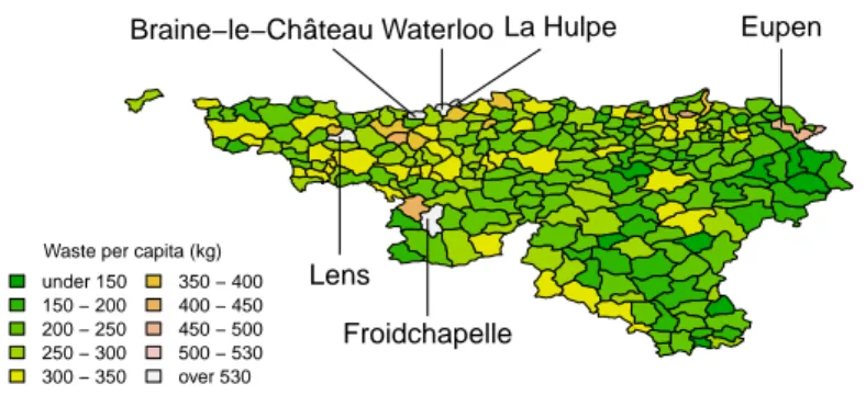
Spatial data may be corrupted by atypical observations and following Haslett et al. (1991), one usually distinguishes two types of outliers. An observation might be an outlier in the traditional way, i.e., it lies far from the majority of the other data points in the space of the non-spatial attributes. In spatial statistics, such an observation is called a global outlier. An observation might also simply have non-spatial attributes with significantly differing values with respect to its neighbours. Such an observation is a local outlier. A local outlier might also be global. The observations can then be categorized into four groups: the local outliers, the global outliers, the local and global outliers and the regular observations. In practice, it is important to be able to identify these four groups. To illustrate these various types of outliers in spatial data, let us consider a real example in one dimension. The amount
Finally, Eupen is a local outlier but not a global one; its observed value is coloured in pink while the values of the surrounding municipalities are coloured in green.
Waste per capita (kg) under 150 150 − 200 200 − 250 250 − 300 300 − 350 350 − 400 400 − 450 450 − 500 500 − 530 over 530 Lens Waterloo La Hulpe Froidchapelle Eupen Braine−le−Château
Figure 1.1: Illustration of local and global outliers in a univariate setting using waste per capita (kg) in Walloon municipalities: Braine-le-Château (global and local), Eupen (local), Froidchapelle (global), La Hulpe (global), Lens (global) and Waterloo (global).
Detecting global outliers is usually performed by means of classical detection tech-niques, like those using Mahalanobis-type distances based on robust estimations of location and covariance. This part of the detection problem is not further discussed. Instead, focus is on the local detection. Schubert et al. (2014) reviewed the local detection techniques available in the literature, with a particular emphasis on spatial data. However, in their Section 5.6, they stress that most known techniques are only able to detect local outliers when a single non-spatial attribute is observed. However, they mention that the methods advocated by Sun and Chawla (2004) and Chawla and Sun (2006) might be applied in the multivariate case even though these authors did not clearly acknowledge that fact. Moreover, the detection technique LOF and its variants, that are fully described in Schubert et al. (2014), are illustrated in the multivariate setting in Breunig et al. (2000) and widely available in the R package dprep. Other local detection techniques exist and may be applied in the multivariate case. Indeed, Chen et al. (2008), Filzmoser et al. (2014) and Harris et al. (2014), all develop detection techniques applicable to multivariate non-spatial attributes, but
these were not considered in the review of Schubert et al. (2014). Therefore, the main aim of this chapter is to provide a complement to the paper of Schubert et al. (2014) by expressing these known multivariate methods along the lines of the general framework based on the context and model functions introduced in Schubert et al. (2014). The literature review stretches to 2016, the year of submission of our paper Ernst and Haesbroeck (2017). The papers published afterwards are discussed in the conclusion. In parallel, a second contribution is to slightly adapt the procedure of Filzmoser et al. (2014) in order to increase its local characteristics. The main ad-vantage of the adapted procedure is to improve the exploratory analysis of data by providing additional insights on the detected local outliers.
More specifically, Section 1.2 reviews the existing multivariate local techniques following Schubert et al. (2014)’s approach while Section 1.3 describes the local adap-tations that can be applied to Filzmoser et al.’s technique in order to improve its local nature. Then, the different proposals are compared by means of real data examples (Section 1.4) and by means of simulations (Section 1.5). Some conclusions follow in Section 1.6.
1.2
Local detection in spatial data
Schubert et al. (2014) decompose any local detection procedure in basically two steps: first, a kind of outlyingness measure (typically a distance) is computed for each spatial unit and secondly, this measure is compared with those computed on other spatial units to decide whether it is outstanding.
Schubert et al. (2014) describe the computation of the outlyingness measure by means of a model function which is applied on a possibly restricted set of observations (usually the neighbours of the spatial unit under consideration). This subset of data points is called the context set and when it does not contain all the data points, the outlyingness measure has a local flavor. In the outlier detection technique reviewed by Schubert et al. (2014), most (but not all) context sets are local.
The comparison step, performed by means of a comparison function, is based on the measures derived on a given set of units, this set being possibly different from the set of neighbours. In Schubert et al. (2014) terminology, this other subset is called the reference set. It might contain all the data points (yielding a global comparison) or a subset of these (corresponding to a local comparison). At the end of the process, the
techniques resulting on a binary classification, we do not consider this additional refinement of the process.
In order to describe the two-step components of the multivariate local detection techniques outlined in the Introduction, some definitions and notations need to be
introduced. Let z1, . . . , zn denote the p-dimensional observations associated with
some spatial coordinates s1, . . . , sn, i.e., zi is the observed value of Z(si) where Z
is a p-variate random vector. Focusing on local outlyingness requires to define a
neighbourhood for each observation. Let Nidenote the neighbourhood of the location
si, 1 ≤ i ≤ n. Any type of neighbourhood might be considered since, following
Schubert et al. (2014)’s philosophy, the choice of the neighbourhood should be made independently from the choice of the detection technique. For instance, it could be decided to construct neighbourhoods containing a fixed number of observations, k
say, the observations selected in Ni being the k − 1 nearest neighbours of si. The
closeness is assessed by means of an appropriate distance (e.g. Euclidean distance or orthodromic track) computed on the spatial coordinates. To keep the choice of
the neighbourhoods unspecified, the number of neighbours in Ni is denoted as ni
throughout the text.
Most techniques compute, at some point in their process, a Mahalanobis-type distance. Let µ and Σ denote respectively a p-dimensional vector (a center) and a p × p positive-definite matrix (a variance-covariance structure) and consider a
p-variate observation z. The squared distance between z and µ while taking into
account the correlation structure inherent to Σ is denoted as
dµ,Σ(z) = (z − µ)TΣ−1(z − µ).
In practice, estimations of µ and Σ are required in order to compute these distances. Classically, the sample mean and covariance matrix are used but, in a perspective of outlier detection, robust alternatives should be favored. All the techniques re-viewed in this section rely on the Minimum Covariance Determinant (MCD)
estima-tor (Rousseeuw, 1985). For a random sample {z1, ..., zn}, with zi ∈ IRp, the MCD
estimator is determined by selecting a subset of h observations (with n/2 ≤ h ≤ n) which minimizes the generalized variance among all possible subsets of size h. The MCD location and scatter estimations are then given by the sample mean and the sample covariance computed from this subset.
Following a similar presentation as in Table 4 of Schubert et al. (2014), here is now the description of the context and reference steps of the three listed multivariate techniques.
1. Median Algorithm, (Chen, Lu, Kou, and Chen, 2008)
This proposal is a multivariate extension of the univariate approach (described also in Chen et al., 2008, but already introduced in Lu et al., 2004) based on the detection of the outlying distances computed between the observed non-spatial attribute of a spatial unit and the median of that attribute over its neighbours.
Context Model function
Ni Computation of hi which is the difference (in IRp)
be-tween zi and the vector of marginal medians computed
on zj with sj ∈ Ni.
Reference Comparison function
Global Computation of the distances dµ, ˆˆΣ(hi), 1 ≤ i ≤ n,
where ˆµ and ˆΣ are the MCD location and dispersion
estimators computed on h1, . . . , hn.
Comparison of these distances with a F -quantile.
2. Detection technique of Filzmoser, Ruiz-Gazen, and Thomas-Agnan (2014) In some cases, as explained by Schubert et al. (2014), the context or the com-parison steps might be divided into several sub-steps, not based on the same context or reference sets. This happens in the approach of Filzmoser et al. (2014) as a global estimation step needs to be carried out before working inside each neighbourhood.
Context Model function
Global Robust estimation of the center and dispersion of
{z1, . . . , zn} by means of the MCD estimator; yielding
ˆ µ and ˆΣ.
Ni Computation of the nidistances dzi, ˆΣ(zj) with sj ∈ Ni.
Computation of the isolation degree of si.
Reference Comparison function
Global Comparison of the isolation degrees and selection of the
Context Model function
Global (optional) Reduction of the dimension with robust PCA.
Ni Application of a Geographically Weighted PCA in Ni
Computation of score distances (SD), orthogonal dis-tances (OS) and component scores (CS).
Reference Comparison function
Global Comparison of the univariate measures SD, OS, and
CS with theoretical quantiles or empirical quantiles.
One can see that all methods work locally, at least partially, for the context part of the procedure while the comparison step is operated on a global level. The number of steps performed on a local level yields the so-called degree of locality of the search procedure, as defined in Schubert et al. (2014). The above techniques have a single local step in their process. Let us note also that Harris et al. (2014) as well as Filzmoser et al. (2014) distinguish local and global outliers and separate the search of the two types of outliers. Only the local detection is taken into account in the description here. Chen et al. (2008) do not mention the different types of outliers and detect all of them indifferently.
The local nature of the detection technique of Filzmoser et al. (2014) is restricted to a single step and this local step is preceded by a preliminary global step in order to compute the overall correlation structure of the data. Transforming this initial step into a local one is one of the elements implemented in the adaptation, as outlined in the next section.
1.3
Local adaptation of the detection technique of
Filzmoser et al. (2014)
1.3.1
Local structure
In Filzmoser et al. (2014), the model function used in the neighbourhood Ni is
based on the computation of the pairwise squared distances
dz
i, ˆΣ(zj) = (zj− zi)
TΣˆ−1(z
j− zi) with sj∈ Ni (1.1)
which rely on the robust estimation of the global correlation structure. The global correlation structure (as well as the global center ˆµ) is also at the core of the
com-putation of the isolation degree as this degree is a quantile of a decentralized χ2
distribution with non-centrality parameter given by dµ, ˆˆΣ(zi). Using the same
over-all structure implicitly assumes that the data are stationary, but may prove to be inefficient when the neighbourhoods have different shapes.
Therefore, in order to increase the local nature of the procedure, we suggest to plug locally estimated covariance matrices into the definition of the pairwise squared distances (1.1), yielding so-called local squared distances
dz
i, ˆΣi(zj) = (zj− zi)
TΣˆ−1
i (zj− zi) with sj∈ Ni
where ˆΣiis estimated using only the attribute values of the statistical units belonging
to Ni∪ {si}. Now, some care is required in the estimation process as the number of
observations included in each neighbourhood, ni, may be small (typically a fraction
of the sample size) and, in high-dimensional cases, the number of units in Ni∪ {si}
may even be smaller than the dimension p.
To ensure the positive-definiteness of the estimated covariance matrix, using reg-ularized estimators is an option that is suggested in the literature (Witten and Tib-shirani, 2009, Friedman et al., 2008). Moreover, as detection of outliers is at sake here, robustness should also be advocated. Therefore, the regularized version of the Minimum Covariance Determinant estimator outlined in Fritsch et al. (2011) is used for the local and robust estimation of the covariance matrix in each neighbourhood. The regularized MCD estimator is obtained by the maximization of the penalized negative log-likelihood function restricted to a subset of n/2 ≤ h ≤ n observations, i.e., log |Σ| + 1 n X zj∈H (zj− µ)TΣ−1(zj− µ) + λTrΣ−1
As explained in Fritsch et al. (2011), the FAST-MCD algorithm of Rousseeuw and Driessen (1999) may be adapted in order to compute the regularized version of the MCD estimator. As a final remark concerning the use of a robust and regularized estimator in the detection procedure, let us note that it does not relate to the regu-larization step suggested in Kriegel et al. (2011).
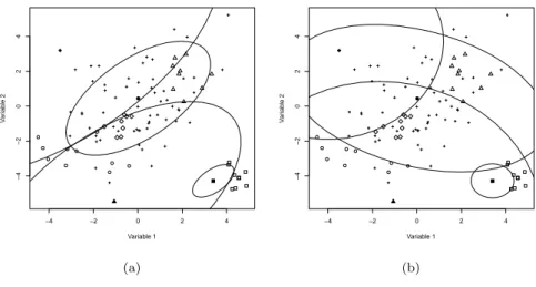
As illustration, let us consider the artificial data set, named dat, of the R pack-age mvoutlier. It consists of n = 100 observations distributed according to the bivariate normal distribution contaminated by some outliers (see the scatter plot of the non-spatial attributes on Figure 1.2). Filzmoser et al. (2014) highlighted the four observations represented by full symbols on Figure 1.2 (panel a). Each of these obser-vations has nine neighbours represented by identical (but empty) symbols. One can see that the full diamond and triangle are local and global outliers, the full circle is a
non-spatial attribute zj lies the closest to zi). On panel b, the same approach is
followed, but this time the structure of the ellipse varies from one point to the next since it is locally estimated by means of the regularized MCD estimator.
−4 −2 0 2 4 −4 −2 0 2 4 Variable 1 V ar iab le 2 (a) −4 −2 0 2 4 −4 −2 0 2 4 Variable 1 V ar iab le 2 (b)
Figure 1.2: Artificial data set dat of the R package mvoutlier: (a) illustration of Filzmoser et al.’s detection technique and (b) illustration of its adaptation.
1.3.2
Restriction to homogeneous neighbourhoods
A second adaptation can be added to the methodology in order to take into account the possible heterogeneity of the attributes of the spatial units included in a given neighbourhood. Indeed, as also stressed in Chawla and Sun (2006), an observation should not be classified as a local outlier if its non-spatial attributes differ from those of its neighbours because they are simply lying in an unstable area. Therefore, only the spatial units whose neighbourhoods consist of spatial units with
non-spatial attributes that are sufficiently concentrated in IRp could be considered
in the detection process.
To measure the concentration in the space of the non-spatial attributes, the vol-ume of the ellipsoid centred at the robust estimation of the local mean, shaped ac-cording to the locally estimated covariance matrix, could be computed. The volume of such an ellipsoid is proportional to the determinant of its structure matrix (the proportionality factor depending only on the dimension p and not on the number of points in the neighbourhood). However, as the sizes of the neighbourhoods might vary, comparing the determinants of the locally estimated covariance matrices is not
appropriate. The ellipsoid must be scaled (inflated or deflated) to make the different cases more comparable.
More precisely, here is the approach that has been followed to measure the con-centration inside the neighbourhoods. Assume that the i-th neighbourhood is under consideration (with sample size ni) and let ˆµi and ˆΣi be the regularized MCD
es-timations derived on zj, sj ∈ Ni∪ {si}. The estimated covariance matrix ˆΣi is
characterized by a given size, i.e., its determinant, and a given shape defined by the matrix ˆVi given by ˆΣi/
p
p
det ˆΣi. Using the shape matrix instead of the covariance
matrix in the construction of the ellipsoids yields ellipsoids of comparable volumes for all the neighbourhoods (as the determinants of all shape matrices are equal to
1). An appropriate measure of concentration in the i-th neighbourhood, cisay, may
then be defined as follows:
ci= 1 hi X j:sj∈Hi dµˆ i, ˆVi(zj)
where Hi is the optimal subset corresponding to the regularized MCD estimations
computed on Ni∪ {si}, this subset containing non-outlying observations by
con-struction. Multiplying the shape matrix ˆVi by ci (which may be interpreted as a
deflation or inflation factor), the volume of the ellipsoid becomes proportional to det(ciVˆi) = c
p
i. Another option for computing this measure of concentration would
be to replace the mean operator by the median, i.e.,
ci = median
j:sj∈Ni
dµˆ
i, ˆVi(zj).
This yields results that are quite similar, as illustrated in Section 1.4.1.
Finally, the resulting volumes, or equivalently the resulting mean squared
dis-tances ci, are then ranked from the smallest (i.e., most concentrated ellipsoid) to
the largest (i.e., the biggest ellipsoid). Only the spatial units having neighbourhoods characterized by a volume ranked among the dβ × ne smallest (for an appropriate value of β as discussed in the next Subsection) are further considered in the local de-tection technique. The set of spatial units selected for the final step of the dede-tection is denoted as D.
1.3.3
Modification of the reference set and of the comparison
χ2distribution is no longer valid. This parametric approach has been replaced by a
non-parametric one using the local distances between each observation and its next neighbour, the next neighbour of a given observation being the neighbour whose non-spatial attributes lie closer to the non-non-spatial attributes of the observation. The closeness is therefore measured in the space of the non-spatial attributes and not in the space of the spatial coordinates. When this distance is large, the corresponding observation is tagged as a local outlier.
In summary, the adapted Filzmoser et al. technique, referred to as the regularized spatial detection technique from now on, might be described by the following steps:
Context Model function
Ni Robust and regularized estimation of the center and
dis-persion of the data {zj, sj ∈ Ni ∪ {si}}; yielding ˆµi and
ˆ Σi.
Computation of the deflation factor ci.
Global Ranking of ci, 1 ≤ i ≤ n, and selection of the units si
corre-sponding to the dβ ×ne most homogeneous neighbourhoods.
Reference Comparison function
Ni with si∈ D Computation of the squared distances of the closest
neigh-bours minsj∈Nidzi, ˆΣi(zj).
D Comparison of the distances and selection of the largest
ones.
Let us observe that there are now two distinct local steps in this procedure, increasing by 1 the degree of locality of the initial procedure.
1.3.4
Tuning parameters
There are several parameters that need to be chosen in order to apply the reg-ularized spatial detection technique. First, the local estimation step requires the tuning of two parameters: the coverage of the MCD estimator (i.e., the number h of observations included in the MCD calculations) and the regularization parameter λ. Then, a fraction β has to be chosen in order to keep only the most concentrated neighbourhoods.
1. Coverage of the regularized MCD estimator
Usually, the coverage is chosen according to the breakdown point one wants to achieve by taking h = dn × (1 − α)e where 0 < α < 1/2 is the chosen breakdown value. The breakdown point is, roughly speaking, the smallest fraction of con-tamination which renders the estimations meaningless. Under regularization,
as the sample size n might be smaller than the dimension p, defining h as above is misleading as p might be bigger than n. In fact, one can show that the break-down point of the regularized MCD estimator is given by min(h, n − h + 1)/n. As it is quite natural not to expect more than 25% of outliers inside each neigh-bourhood, it was decided to set the coverage rate to the proportion 0.75 (i.e.,
hi = d(ni + 1) × 0.75e) for all the local estimations. Of course, to achieve
robustness, it is necessary to have hi< ni+ 1, which is only guaranteed if the
size of the neighbourhood is at least equal to 3. Therefore, spatial units which are quite isolated and have less than three neighbours cannot be considered by the regularized spatial detection technique, unless their neighbourhoods are inflated until reaching the minimum required number of neighbours.
2. Regularization parameter λ
The regularization parameter was locally set following a suggestion outlined in Fritsch et al. (2011). Indeed, as the penalty function considered in their paper is based on the trace of the concentration matrix (the inverse of the covariance matrix), a value of λ equal to trΣ/np would yield an unbiased estimation of the trace of the covariance matrix. Inspired on this idea, λ may be locally set in each neighbourhood to the value dtrΣi/hip where dtrΣi should be robustly
estimated. To do so, it is sufficient to get robust estimations of each marginal
variance. Let ˆσi` denote the marginal median absolute deviation of the `-th
coordinate of Z computed in the ith neighbourhood. Then,Pp
`=1ˆσi`2 does the
job.
3. Homogeneity proportion
As explained above, only the spatial units corresponding to a given proportion (β say) of the most homogeneous neighbourhoods are further analysed in the regularized spatial detection technique. Taking β too large (i.e., keeping spatial units whose neighbours have a heterogeneous pattern) tends to increase the false detection rate. On the other hand, taking β too small might be too restrictive
if some small neighbourhoods contain several local outliers. To enrich the
exploration analysis of the data, we advise to choose a whole range of β values and to visualize the results on adjusted boxplots. More specifically, select a grid
boxplot is defined by
[Q1− 1.5 e−4MCIQR; Q3+ 1.5 e3MCIQR]
where MC denotes the medcouple, which measures the skewness of the sample and is given by MC = median zi≤Q2≤zj (zj− Q2) − (Q2− zi) zj− zi .
The next distance associated with si corresponds to the smallest distance
among the locally estimated squared distances dz
i, ˆΣi(zj), with sj ∈ Ni. The
units having much bigger next distances than the others may then be flagged as local outliers, a natural cutoff being given by the upper whisker of the ad-justed boxplot. The simultaneous consideration of several values of β allows to measure the degree of outlyingness of the observations and to visualize the potential impact the local heterogeneity might have on this outlyingness.
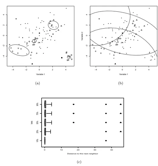
Going back to the artificial data dat of the R package mvoutlier, Figure 1.3 illustrates the effect of the choice of β on the results of the detection. Looking first at the boxplots (panel c), one can see that choosing β = 0.1 (first boxplot) only yields the full diamond as local outlier. When β = 0.25, the full triangle is also classified among the local outliers. Finally, when β ≥ 0.5, a third local outlier (the full circle) appears. The plot on panel a shows that the structure and the homogeneity of the neighbourhoods vary for the different symbols, illustrating the necessity to adjust the structure locally and to focus only on the stable areas. On panel b, the local distance of the closest neighbour is illustrated using the ellipse centred at the observation zi
and inflated until reaching its closest neighbour.
1.4
Examples
In this section, examples already considered in the literature are exploited to com-pare the detection techniques reviewed or introduced in Sections 1.2 and 1.3. All the computations are done in the statistical software R. The detection technique of Filz-moser et al. (2014) was applied via the procedures locoutPercent, locoutneighbor and locoutSort of the package mvoutlier and the outliers are detected visually by means of Filzmoser et al.’s suggested graphical display. The procedure of Harris et al. (2014) was partially re-implemented using, as a core component, the procedure gwpca of the package GWmodel. All the available tools (i.e., the score distances SD, the or-thogonal distances OD and the component scores CS) were computed and compared to empirical quantiles (the theoretical quantiles advocated by Harris et al. (2014) for the two measures SD and OD are too small in most examples, due probably to the non normality of the data). Note that the use of the procedure gwpca restricts the
−4 −2 0 2 4 −4 −2 0 2 4 Variable 1 V ar iab le 2 (a) −4 −2 0 2 4 −4 −2 0 2 4 Variable 1 V ar iab le 2 (b) 10% 25% 50% 75% 90% 0 10 20 30 40
Distance to the next neighbor
beta
(c)
Figure 1.3: Illustration of the regularized spatial detection technique on the artificial data dat of the R package mvoutlier: (a) comparison of the homogeneity of the
application of Harris et al.’s technique to cases where the neighbourhoods contain the same number of neighbours or are constructed by means of a given critical distance. Chen et al. (2008)’s technique was implemented in R as no public procedure could be found.
1.4.1
Social data in France
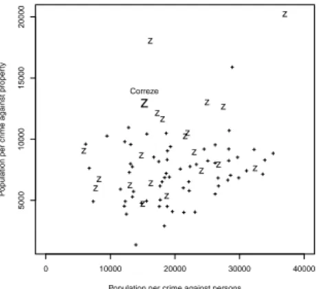
Dray and Jombart (2011) revisited social data measures on 85 departments in France in 1830. The data set is available in the R package Guerry. For illustra-tive reasons, only the two following variables are selected here: population per crime against persons and population per crime against property. Moreover, as in Filz-moser et al. (2014), the neighbourhoods are constructed as the set of the 20 closest neighbours.
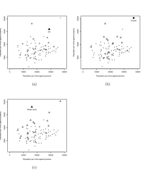
On Figure 1.4 (showing the scatter plot of the two non-spatial attributes), the results obtained by the technique advocated by Chen et al. (2008) is illustrated. The three full symbols represent the three local outliers (Ain, Creuse and Haute-Loire) found by that technique. The corresponding empty symbols highlight their neighbours. There are two worth noting points: first, these outliers clearly lie far from the bulk of the data, implying also a global outlyingness (they are, together with the department of Correze, classified solely as “global” outliers by Filzmoser et al. (2014), as shown on Figure 1.6). Then, the important dispersion among the non-spatial attributes of the neighbours of the detected points questions the relevance of their local outlyingness. The technique of Harris et al. (2014) detects the same three outliers as well as the department of Correze (on Figure 1.5), for which the lack of homogeneity inside the neighbourhoods is again quite visible.
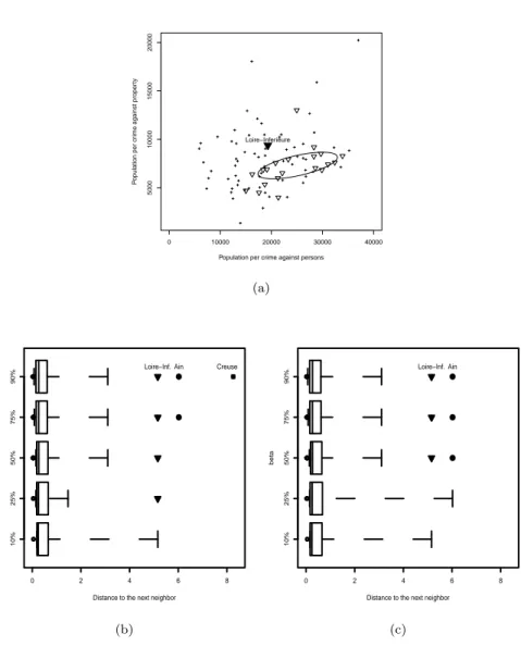
The technique of Filzmoser et al. is illustrated on Figure 1.6 and pinpoints a single local outlier: the Rhone department. Again, one may argue that Rhone is maybe not so outlying when one takes into account the dispersion inside its neighborhood. In fact, it turns out that the homogeneity is quite weak inside each neighbourhood, implying that the notion of local outlyingness is not so clear for that particular data set. Nevertheless, the regularized spatial detection technique detects only one local outlier (Loire Inférieure) when β is set to 0.25. Figure 1.7 (panel a) illustrates the relative homogeneity of the neighbourhood of the detected point while the adapted boxplots (panel b) show that the next distances of the selected point lie outside the outer fences of the box for that particular value of β. If β is set to 0.75 or 0.9, one or two other local outliers (Ain and Creuse) are also detected but their neighbourhoods undoubtedly are heterogeneous. Therefore, one needs to decide whether labelling these observations as local outliers is really appropriate. As explained in Section 1.3.2, the homogeneity measures are based on the computation of the mean of a subgroup of (uncontaminated) local distances, but the median of the local distances
0 10000 20000 30000 40000
5000
10000
15000
20000
Population per crime against persons
P
opulation per cr
ime against proper
ty Ain (a) 0 10000 20000 30000 40000 5000 10000 15000 20000
Population per crime against persons
P
opulation per cr
ime against proper
ty Creuse (b) 0 10000 20000 30000 40000 5000 10000 15000 20000
Population per crime against persons
P
opulation per cr
ime against proper
ty
Haute−Loire
(c)
Figure 1.4: Social data: detection based on Chen et al. (2008). Representation of three “local” outliers and their neighbours. They are clearly global outliers and the
might have been used instead. Panel c of Figure 1.7 illustrates the results obtained for that other option. We can see that the two main local outliers are detected again but at slightly different levels of homogeneity (i.e., at different values of β).
0 10000 20000 30000 40000
5000
10000
15000
20000
Population per crime against persons
P
opulation per cr
ime against proper
ty z Correze z z z z z z z z z z z z z z z z z z z z
Figure 1.5: Observation classified as a local outlier by the technique of Harris et al. (2014) in addition to the three illustrated on Figure 1.4. The neigh-bourhood is quite heterogeneous and the observation is labelled as global outlier for Filzmoser et al. (2014).
0 10000 20000 30000 40000
5000
10000
15000
20000
Population per crime against persons
P
opulation per cr
ime against proper
ty Rhone Ain Creuse Haute−Loire Correze
Figure 1.6: Detection of a local outlier (Rhône) and illustration of the global outliers for the technique of Filzmoser et al. (2014). The local outlyingness of this observation may not be rele-vant considering the dispersion inside its neighbourhood.
1.4.2
Geochemical data
The Baltic Soil Survey data (BSS data, available in the R package mvoutlier) were collected in agricultural soils from Northern Europe (total area of about 1 800
000 km2, 768 sampling sites taken on an irregular grid). Only the ten elements
from the top layer (Al2O3, F e2O3, K2O, M gO, M nO, CaO, T iO2, N a2O, P2O5
and SiO2) are considered here and, after the application of the isometric log-ratio
transformation (as the data are compositional), this yields a dimension p = 9. The neighbourhoods are the same as those constructed by Filzmoser et al. (2014), i.e., they correspond to the sets of the 10 nearest neighbours. With such a small sample size inside the neighbourhoods, the technique of Harris et al. (2014) requires first the application of the global step based on a robust Principal Component Analysis, presented as optional in Section 1.2. Five principal components are kept through the detection process.
0 10000 20000 30000 40000
5000
10000
15000
20000
Population per crime against persons
P
opulation per cr
ime against proper
ty Loire−Inferieure (a) 10% 25% 50% 75% 90% 0 2 4 6 8
Distance to the next neighbor
beta
Loire−Inf. Ain Creuse
(b) 10% 25% 50% 75% 90% 0 2 4 6 8
Distance to the next neighbor
beta
Loire−Inf. Ain
(c)
Figure 1.7: (a) The observation Loire-Inférieure is detected by the regularized spatial detection technique with β = 0.25. The boxplots of “next distances” are given for varying values of β when using the mean of the distances (plot on panel b) or the
Figure 1.8 (panel a), representing the different locations where the data were collected, summarizes the results of the different detection techniques. The most locally outlying spatial units detected by Chen et al. (2008) are plotted as full circles while crosses are used for Filzmoser et al. (2014) and empty squares represent the results of the detection of Harris et al. (2014). Based on the new approach, three local outliers (full triangles) are spotted. It is interesting to note that most outliers found by Chen et al. (2008), Harris et al. (2014) and Filzmoser et al. (2014) do not belong to the set D of spatial units lying in the most homogeneous areas and could not therefore be pointed out by the spatial regularized technique. Moreover, once again, the local outliers pinpointed by Chen et al. (2008) would be tagged as global by the full detection technique of Filzmoser et al. (2014).
+
+ +
(a) (b)
Figure 1.8: Detection of local outliers on geochemical data measures in Northern Europe. (a) Detected local outliers for each technique: full circle (Chen et al., 2008), crosses (Filzmoser et al., 2014), empty squares (Harris et al., 2014) and full triangles (regularized spatial detection technique). (b) The swapping of these two highlighted observations is entirely detected by the regularized spatial technique but not by the others.
To further analyze the performance of their detection techniques, Filzmoser et al. (2014) contaminated the data by exchanging the non-spatial attributes of two spatial units. Their contamination is not detected by Chen et al. (2008) nor by Harris et al.
(2014) and by the regularized spatial technique, as the considered neighbourhoods do not belong to the homogeneous set D. However, swapping the observations obtained at the two locations highlighted on panel b of Figure 1.8 makes Filzmoser et al. (2014) detection partially fail (as it detects only one of the local outliers) while the regularized spatial technique works fine. The swapping of these two locations is based on a “contamination” technique advocated by Harris et al. (2014). A robust Principal Component Analysis is applied on the non-spatial attributes and the observations of D with the smallest score and the largest score on the first principal component are swapped. This contamination procedure is used again in the simulation study (see Section 1.5).
1.4.3
Cancer data in France
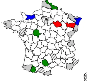
This data set contains five variables: the male lung cancer mortality rate (stan-dardized over the age range 35–74 and over the 2-year period, 1968–1969), the cigarette sales and the percentages of employed males in specific types of industry (metal, mechanic and textile), the variables being measured at the scale of 82 French departments. These data come from Richardson et al. (1992). This time, following Richardson et al.’s way of proceeding, two departments are considered neighbours if they share a boundary. This implies that the spatial units get different numbers of neighbours (numbers ranging from one to eight). As the regularized detection technique requires at least three observations in order to estimate the local structure in the neighbourhoods, the nine departments having only one or two neighbours are neglected in the detection analysis, but they are kept when playing the role of neigh-bour for another spatial unit. Also, a second limitation in the study of this data set comes from the fact that Harris et al.’s procedure cannot be applied as currently implemented because the neighbourhoods have varying sizes and are not defined in terms of a critical distance. Therefore, only the three other techniques are considered. These techniques detect different outlying departments as illustrated on the map of France in Figure 1.9: Vosges (which has six neighbours) and Aube (with five neighbours) for Chen et al. (2008); Bas-Rhin and Calvados (both having three
neigh-bours) for Filzmoser et al. (2014); Nord (ni= 3, β ≥ 0.25), Hautes-Pyrénées (ni= 3,
β ≥ 0.25), Indre-et-Loire (ni = 5 and β ≥ 0.25) and Tarn (ni = 5, β = 0.5) for the
Figure 1.9: Map of France with outlying departments colored in red (Chen et al., 2008), blue (Filzmoser et al., 2014) or green (Regularized spatial technique). The grey-shaded areas represent those departments excluded from the detection proce-dure. In the data set, the hatched departments are not included and the dotted ones around Paris are aggregated.
1.4.4
Preliminary conclusion
As a preliminary conclusion, one might say that it is difficult, using real data, to put forward a detection technique which performs best. Indeed, it is not clear which observations are really locally outlying and most detected observations are different using one technique or another. The next section resorts to simulations to get a more objective comparison, local outliers being known in advance as they are inserted in clean data sets.
Nevertheless, most examples illustrate the fact that Chen et al. (2008)’s proce-dure mixes up global and local outliers. Another comment is the fact that the new regularized spatial detection technique gives additional insights on the outlyingness of the observations thanks to the possible consideration of several values of β. Using a fixed and unique value of β might be a bit too restrictive as one would then focus
only on a subsample of potential outliers (only on those lying in the most homo-geneous neighbourhoods). Most local outliers found by the other techniques would not be found by the new procedure if restricted to the β × 100% most homogeneous neighbourhoods for a fixed β. We recommend to vary the values of β and to keep in mind the corresponding interpretation. When using the other techniques, one needs to decide whether a spatial unit living in an unstable area should really be tagged as a local outlier. Finally, it is worth stressing once again that the first step of the regularized spatial detection technique is local, even if the sample size of the neighbourhoods is small (possibly smaller than the dimension) while the detection technique of Filzmoser et al. (2014) starts with a global estimation step (avoiding the local problem) and that of Harris et al. (2014) requires the application of an additional global step to handle data sets where the dimension is big.
1.5
Simulations
In this section, simulations are conducted in order to provide an objective
com-parison of the three detection techniques reviewed in Section 1.2. As additional
information, the impact of the suggested adaptations presented in Section 1.3 is analysed. Harris et al. (2014) had already resorted to simulations, but with the sole objective of comparing variants (theoretical or empirical quantiles as cutoffs, differ-ent construction of the weight matrix inducing the neighbourhoods,...) of their own technique. Therefore, their simulation study is extended here to envelop the other detection techniques as well, while using only their default proposal instead of all their variants (i.e., theoretical quantiles are used as cutoffs for the measures SD and OD while empirical quantiles are computed for CS and the neighbourhoods are based on a given number of closest neighbours). In Section 1.4 devoted to the examples, the local outliers detected by Filzmoser et al.’s technique (as well as by its adaptation) are found by means of the visual analysis of some graphical displays. In simulations, this visual detection is no longer possible and needs to be automated. Filzmoser et al.’s procedure is automated as follows: when the isolation degree is three times bigger than the expected value (taken equal to 1/k where k is the number of neigh-bours), then the observation is tagged as a local outlier. For the regularized spatial detection technique, observing the changes for varying values of β and globalizing the detection is the best option. In the simulations, the search is decomposed into
Hubert and Vandervieren (2008) are tagged as local outliers for that specific β. To perform simulations in a spatial context, one needs to define the spatial units as well as a spatial correlation structure for the non-spatial attributes. Also, as outlier detection is the main interest here, contamination has to be introduced in the data. Finally, an objective way to measure the performance of the detection techniques should be defined. The choices made for these four aspects of the simulation study are further developed in the following subsections. Then, the results are outlined and discussed.
1.5.1
Spatial units
To mimick a practical situation, adapting Harris et al.’s idea to the Belgian set-ting, the first round of simulations is performed on spatial units consisting of the n = 262 municipalities of the Walloon region in Belgium (the municipalities, char-acterized by their longitude and latitude, are already illustrated in Figure 1.1 and may be visualized again on the different panels of Figure 1.10). In parallel, a more rigid configuration consisting of a 20 × 20-cell grid is considered for a second set
of simulations. In both cases, neighbourhoods are constructed by means of the
ni = k = [0.05 × n] closest neighbours (even for the cells lying at the border of
the square). Of course, in the grid case, the neighbourhoods show a more regular pattern than in the case of Wallonia.
1.5.2
Spatial correlation structure
The simulated data come from a p-dimensional Gaussian and second-order sta-tionary process with mean vector zero and covariance matrix given by, following the notations of Gneiting et al. (2010),
C(h) = C11(h) . . . C1p(h) .. . . .. ... Cp1(h) . . . Cpp(h) with Cii(h) = σi2M (h|ν, a), i = 1, . . . , p and Cij(h) = ρijσiσjM (h|ν, a), i, j = 1, . . . , p (i 6= j)
where M (h|ν, a) is the spatial correlation at a distance h based on the Matérn func-tion. The restriction to a constant spatial scale parameter a and a constant smooth-ness parameter ν yields the so-called parsimonious multivariate Matérn model, as already used by Harris et al. (2014). Consistently with the purpose of extending
their results, similar values for the tuning parameters a and ν and for the elements of the cross-covariance matrix, ρij, 1 ≤ i, j ≤ p and σi, 1 ≤ i ≤ p, are chosen. First, the
spatial scale parameter is set to 1. Then, for p = 5, the following cross-covariances and variances is used:
Σ = 70 60 60 65 65 60 90 75 70 70 60 75 95 60 55 65 70 60 75 60 65 70 55 60 85
where Σij = ρijσiσj with ρii = 1 ∀ i. For smaller values of the dimension p, the
upper-left p × p square sub-matrix of Σ is chosen.
As far as the smoothness parameter is concerned, note first that larger values correspond to smoother variations. The choice of ν is illustrated in the bivariate case in Figure 1.10 using the real spatial locations of the Walloon municipalities. On the two upper panels, ν is set to 0.5, while it is equal to 2.5 (value suggested in Harris et al., 2014) on the lower panels. Both choices are further considered in the simulation study as, to our point of view, they provide different homogeneity patterns even though, for each case separately, the neighbourhoods have comparable homogeneity. Under such a scheme, restricting the detection to a small number of the most homogeneous neighbourhoods is counterproductive. This explains why β is set to values above 40% in the simulations.
1.5.3
Contamination set-up
Simulating the data by means of the Gaussian and second-order stationary process detailed above should yield data free of local outliers. Global outliers are possible though, but these are not under consideration here (unless they are local at the same time). As introduced in the example of Subsection 1.4.2, the contamination process defined in Harris et al. (2014) is used for the simulations. In order to reach a given percentage of local contamination, 5% say, more care needs to be given to the construction of these local outliers. Indeed, as already stressed by Harris et al. (2014), it may happen that, as suggested, the contamination method ends up with the swap of a bunch of neighbours. If they have close attributes in the beginning and are swapped all together, they keep similar values and cannot be considered local
Variable 1 Variable 2
Variable 1 Variable 2
Figure 1.10: Gaussian and second-order stationary process based on the parsimonious Matérn model for ν = 0.5 (upper panels) and ν = 2.5 (lower panels) to illustrate different homogeneity patterns.
on panel b. Clearly, patches of neighbours are swapped without introducing the expected 5% of local contamination in the data.
Harris et al. (2014) solve this problem by not focusing on the highest and low-est scores. Here, another way of choosing the units that will be swapped has been designed. Again, the highest scores correspond to potential candidates to swap with the smallest ones, but the selection proceeds one at a time and discards any spatial unit lying in the neighbourhood of another one which was previously selected. For the clean set-up illustrated on Figure 1.11 (panel a), this adaptation of Harris et al.’s proposal yields the contaminated configuration on panel c, where the patches of outliers have disappeared. Unlike in the geochemical application where the contami-nation step is restricted to units lying in D, the local outlier inserted in the simulated data sets might lie in more heterogeneous neighbourhoods.
1.5.4
Performance measure
To measure the performance of a local outlier detection technique, misclassifica-tion error rates may be computed. A good detecmisclassifica-tion technique should not only detect the local outliers, but also avoid to falsely detect good observations as local outliers. The concepts of “false positive” (i.e., a regular observation classified as a local outlier)
−20 −10 0 10 20 −20 −10 0 10 0 2 4 6 8 10 0 2 4 6 8 10 variable1 0 2 4 6 8 10 variable2 coords.x1 coords .x2 (a) −20 −10 0 10 20 −20 −10 0 10 0 2 4 6 8 10 0 2 4 6 8 10 variable1 0 2 4 6 8 10 variable2 coords.x1 coords .x2 (b) −20 −10 0 10 20 −20 −10 0 10 0 2 4 6 8 10 0 2 4 6 8 10 variable1 0 2 4 6 8 10 variable2 coords.x1 coords .x2 (c)
Figure 1.11: Clean (panel a) and 5%-contaminated (panels b and c) 2-dimensional Gaussian process on the grid; (b) the contamination procedure is unrestricted and (c) the contamination has the additional constraint of discarding neighbours.
and “false negative” (i.e., a local outlier which remains undetected) are informative for that matter. Table 1.1, built following Cerioli and Farcomeni (2011)’s notations, summarizes the possible combinations of the outcomes of the detection technique (regular/outlier) with respect to the real category of the data points.
Table 1.1: Contingency table of the real category of the observations with respect to the classification resulting from the application of an outlier detection technique.
Classified as
Reality Regular Outlier Total
Regular T N F P M0
Outlier F N T P M1
Total n − R R n
Several summary measures based on the false positive and false negative error rates are listed in Cerioli and Farcomeni (2011). Here, referring to the notations used in Table 1.1, the performance measures that is computed over the simulations are the false positive error rate defined by F P/M0, the false negative error rate given
1.5.5
Results
For p = 2 and p = 5, 500 data sets were simulated according to the spatial model detailed above, using both the regular grid and Wallonia as spatial domains and using the two specified values for the smoothness parameter (ν = 0.5 and ν = 2.5). The three techniques, as well as the adaptation of Filzmoser et al.’s technique (via four independent applications in order to compare the different β values), were applied to each simulated data set and the three summary measures were recorded for each as well.
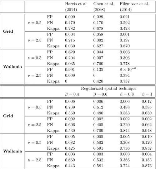
Figure 1.12 shows, using boxplots, the results of the computation on the 500 simulated data sets of the false positive, false negative error rates and of the Kappa measures, under the 2D configuration (using the two spatial domains and for the two ν values), while Figure 1.13 yields the same results for the 5D set-up. Tables 1.2 (for p = 2) and 1.3 (for p = 5) provides the averages of these three summary measures computed over the 500 runs.
Let us first look at the results concerning the false positive error rates. One can see that, whatever the dimension, the technique of Harris et al. (2014) wrongly flags too many good observations as local outliers; the percentage of false positives is only approximately under control when the regular grid with ν = 0.5 is exploited. In the three other settings, the average false positive error rates are well above 50% and the boxplots lie in the upper part of the figures. Chen et al. (2008)’s technique does a bit better, even though it does not handle so well the Wallonia spatial domain with ν = 2.5. The two remaining techniques perform well on that criterion whatever the dimension. It is interesting to note (but not surprising) that there is not any effect of the choice of β on that summary measure (except when all neighbourhoods are searched, in which case the false positive error rate increases a bit).
As far as the false negative error rates are concerned, Chen et al. (2008)’s pro-cedure yields the best results. Its boxplots lie below the others and may even be completely degenerated at 0 in some configurations (meaning that all local outliers are found). The other techniques seem to partially suffer from some masking effect as not all local outliers are detected on average. The detection method of Harris et al. (2014) corresponds to the second best option on that criterion, while the reg-ularized spatial detection technique discarding at least 40% of the neighbourhoods is clearly the worst, which is expected as the contamination was not restricted to the most homogeneous neighbourhoods. Nevertheless, taking β = 0.8 provides more protection against the masking effect and ends up with comparable results with re-spect to Filzmoser et al. (2014)’s technique. This large value of β can be justified by the strong homogeneity of all neighbourhoods obtained by the Gaussian process. Therefore, working only on a small proportion of neighbourhoods (which might be illuminating in real data analysis) is too restrictive in this simulated set-up.