Report on extrapolated time trends at test sites

Texte intégral

(1)Project no. 505428 (GOCE). AquaTerra Integrated Modelling of the river-sediment-soil-groundwater system; advanced tools for the management of catchment areas and river basins in the context of global change. Integrated Project Thematic Priority: Sustainable development, global change and ecosystems Deliverable No.: TREND2.4. Title: Report on extrapolated time trends at test sites Due date of deliverable: November 2005 Actual submission date: November 2005 Start date of project: 01 June 2004. Duration: 60 months. Organisation name and contact of lead contractor and other contributing partners for this deliverable: Broers H.P1, Visser A.2,(eds.) Pinault J.-L.3, Guyonnet D.3, Dubus I.G.3, Baran N.3, Gutierrez A.3 & Mouvet C3 Batlle Aguilar J.4, Ph. Orban4, Brouyere S.4. 1 Netherlands Organisation for Applied Scientific Research TNO, Division Groundwater and Soil, Princetonlaan 6, P.O. Box 80015, 3508 TA Utrecht, The Netherlands. E-mail: h.broers@tno.nl (lead partner) 2 Universiteit Utrecht, Faculty of Geographical Sciences, Budapestlaan 4, 3584 CD Utrecht, The Netherlands. 3 BRGM, Water Division, BP 6009, 45060 Orléans Cedex 2, France. 4 GEOMAC, University of Liege, Building B52/3, 4000 Sart Tilman, Belgium.. Revision: M.H. Gerzabek / J.Barth Project co-funded by the European Commission within the Sixth Framework Programme (2002-2006) Dissemination Level PU Public X PP Restricted to other programme participants (including the Commission Services) RE Restricted to a group specified by the consortium (including the Commission Services) CO Confidential, only for members of the consortium (including the Commission Services).

(2) SUMMARY The establishment of tools for trends analysis in groundwater is essential for the prediction and evaluation of measures taken within context of the Water Framework Directive and the draft Groundwater Directive. This report describes the development of trend detection and extrapolation methods. A novel approach for demonstrating trends is presented for the Dutch Meuse case, based on back-scaling of time series using 3H/3He ages. The method yields convincing results, because it effectively reduces uncertainty in trend analysis, which is caused by groundwater age variations. Trend reversal was demonstrated for several chemical indicators and trend extrapolation was feasible using additional simple regression. The Wallonian Meuse case focuses on the complications caused by more-yearly fluctuations of nitrate in areas with thick unsaturated zones. A comparison was made between parametrical and non-parametrical methods to overcome these inherent sources of variability. Several innovative approaches are presented for the Brévilles catchment in France. Especially the impulse-response approach and the possibilistic regression approach helped to understand the functioning of the groundwater system with respect to pesticide transport. Advantages of these approaches are that the require only information on high temporal resolution monitoring data and rainfall inputs.. MILESTONES REACHED T2.4: Statistical time trend estimation and extrapolation at test locations The extrapolated trends in groundwater seems to be interesting for surface water – groundwater interaction studies in work packages FLUX and BASIN. The effective demonstration of trend reversal in groundwater due to effective Manure regulations in the lower Meuse basin is interesting within the work of EUPOL..

(3) Table of Contents INTRODUCTION TO TREND 2 (TNO) .........................................................................1 1.1 Background and objectives ..................................................................................1 1.2 General methods used in TREND 2.....................................................................2 1.3 TREND 2 case studies.........................................................................................3 1.4 Contents of the current report ..............................................................................3 1.5 Structure of the report ..........................................................................................3 1.6 Glossary ...............................................................................................................4 2. DEMONSTRATING TREND REVERSAL USING TRITIUM-HELIUM AGE SCALING: RESULTS FOR THE DUTCH MEUSE SUBCATCHMENT (TNO/UU).........................5 2.1 Introduction ..........................................................................................................5 2.2 Data......................................................................................................................7 2.3 Back-scaling of time series ..................................................................................8 2.4 Trend extrapolation ............................................................................................12 3. POINT BY POINT STATISTICAL TREND ANALYSIS AND EXTRAPOLED TIME TRENDS AT TEST SITES IN THE MEUSE BE (ULG) ..............................................18 3.1 Introduction ........................................................................................................18 3.2 Description of the dataset of nitrate measurements...........................................18 3.3 Statistical trend analysis.....................................................................................25 3.4 General conclusions and perspectives ..............................................................37 3.5 Appendix ............................................................................................................38 4. CONVENTIONAL AND INNOVATIVE APPROACHES TO TRENDS ANALYSIS: A CASE STUDY FOR THE BRÉVILLES CATCHMENT (BRGM) .................................39 4.1 Introduction ........................................................................................................39 4.2 Time series analysis using 'classical' statistics ..................................................40 4.3 Time series analysis using TEMPO ...................................................................46 4.4 Time series analysis using possibilistic regression ............................................62 4.4 Discrepancy between the CFC age of interstitial water and the mean transfer time calculated from impulse responses........................................................68 4.5 Summary and perspectives................................................................................69 5. DISCUSSION..............................................................................................................71 5.1 Differences between study sites: pumping wells and springs versus observation wells.........................................................................................................71 5.2 Specific results ...................................................................................................73 6. REFERENCES............................................................................................................75 APPENDICES ........................................................................................................................78 1..

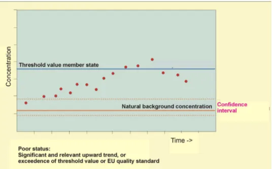
(4) 1. 1.1. Introduction to TREND 2 (TNO). Background and objectives. The implementation of the EU Water Framework Directive (2000/60/EU) and the draft Groundwater Directive asks for specific methods to detect the presence of long-term anthropogenically induced upward trends in the concentration of pollutants in groundwater. Specific goals for trend detection have been under discussion during the preparation of the recent draft of the Groundwater Directive. The draft Directive defines criteria for the identification and reversal of significant and sustained upward trends and for the definition of starting points for trend reversal. Figure 3.1.1 illustrates the trend reversal concept, as communicated by EU Commission Officer Mr. Ph. Quevauviller. The figure 3.shows how the significance of trends is related to threshold concentrations which should be defined by the member states.. Figure 1.1 Trend reversal concept of the draft EU Groundwater Directive.. Trends should be reversed when concentrations increase up to 75% of the threshold concentration. Member states should reverse trends which present a significant risk of harm to associated aquatic ecosystems, directly dependent terrestrial ecosystems, human health, whether actual or poten tial, of the water environment, through the program of measures referred to in Article 11 of the Water Framework Directive, in order to progressively reduce pollution of groundwater. Thus, there is a direct link between trends in groundwater and the status and trends in related surface waters. This notion is central to the overall objectives of Working hypothesis 1: Groundwater quality is of utmost importance to the quality of surface waters. Establishment of trends in groundwater is essential for prediction and evaluation of measures taken within the Framework Directive and the draft Groundwater Directive. the AQUATERRA research project. Accordingly, the work package TREND-2 of Aquaterra is dedicated to the following overall objectives.. Deliverable T2.4, final draft, December 1st. 1.

(5) Development of operational methods to assess, quantify and extrapolate trends in groundwater systems. The methods will be applied and tested at various scales and in various hydrogeological situations. The methods applied should be related to the trend objectives of the Water Framework Directive and draft Groundwater Directive. In addition to the DOW, it is our ambition to link changes in groundwater quality to changes in surface water quality. Linking changes in land use, climate and contamination history to changes in groundwater chemistry. We define a temporal trend as ‘a change in groundwater quality over a specific period in time, over a given region, which is related to land use or water quality management’, according to Loftis 1991, 1996. It should be noted that trends in groundwater quality time series are difficult to detect because of (1) the long travel times involved, (2) possible obscuring or attenuating effect of physical and chemical processes, (3) spatial variability of the subsurface, inputs and hydrological conditions and (4) short-term natural variability of groundwater quality time series. The TREND 2 package is dedicated to the development and validation of methods which overcome many of these problems. Working hypothesis 2: Detection of trends in groundwater is complicated by spatial variations in pressures, in flow paths and groundwater age, in chemical reactivity of groundwater bodies, and by temporal variations due to climatological factors. Methods for trend detection should be robust in dealing with this inherent variability. Groundwater pollution is caused by both point and diffuse sources. Large scale groundwater quality, however, is mainly connected to diffuse sources, so that the TREND 2 project will concentrate on trends in groundwater quality connected to diffuse inputs, notably nutrients, metals and pesticides. We will consider a number of large basins in Europe and try to devise a trend monitoring method and network. Although trends in groundwater quality can occur at large scales, linking groundwater quality to land use and contamination history requires analysis at smaller scale, i.e. groundwater subsystems. Thus, the approach zooms in on groundwater system analysis around observation locations. Results will be extended to large scale monitoring.. 1.2. General methods used in TREND 2. Research activities within TREND 2 focus on the following issues: Inventory of monitoring data of different basins and sub-catchments. The inventory focuses on observation points with existing long time series. The wells should preferably be located in agricultural areas, because pesticides and nutrients are the main concern in trend detection for the Water Framework Directive. Additional information will be collected about historical land use changes and related changes in the input of solutes into the groundwater system. Development of suitable trend detection concepts. Trend detection concepts include both statistical approaches (classical parametrical and non-parametrical methods, hybrid techniques) and conceptual approaches (time-depth transformation, age dating) Methods for trend aggregation for groundwater bodies. The Water Framework Directive demands that trends for individual points are aggregated on the spatial scale of the groundwater bodies. The project will focus on robust methods for trend aggregation. Trend extrapolation. Trend extrapolation will be based on statistical extrapolation methods and on deterministic modelling. Both 1D and 3D model may be applied to predict future changes and to compare these with measured data from time series. Recommendations for monitoring. Results from the various case studies will be used to outline recommendations for optimizing monitoring networks for trend analysis. Deliverable T2.4, final draft, December 1st. 2.

(6) 1.3. TREND 2 case studies. The following case studies have been selected for testing the methodologies: Table 1.1: Case studies Basin Meuse Dommel upper tributaries Noord-Brabant region Wallonian catchments: Néblon Pays Herve Hesbaye Floodplain Meuse Brévilles Brévilles catchment Elbe Czech subbasins Schleswig-Holstein. Contaminants. Institutes. Nitrate, sulfate, Ni, Cu, Zn, Cd Nitrate, sulfate, Ni, Cu, Zn, Cd Nitrate. TNO/UU TNO/UU Ulg. Pesticides. BRGM IETU. Nitrate Nitrate. These cases have different spatial scales and different hydrogeological situations. Details on the various cases are provided in the subsequent chapters of this report.. 1.4. Contents of the current report. This report describes the results of trend analysis, including both trend detection and trend extrapolation. A novel approach for demonstrating trends is presented for the Dutch case, based on back-scaling of time series using 3H/3He ages. The method yields convincing results, because it effectively reduces uncertainty in trend analysis which is caused by groundwater age variations. Trend reversal was demonstrated for several chemical indicators and trend extrapolation was feasible using additional simple regression. The Wallonian case focuses on the complications caused by moreyearly fluctuations of nitrate in areas with thick unsaturated zones. A comparison was made between parametrical and non-parametrical methods to overcome these inherent sources of variability. Several innovative approaches are presented for the Brévilles catchment in France. Especially the impulse-response approach and the possibilistic regression approach helped to understand the functioning of the groundwater system with respect to pesticide transport.. 1.5. Structure of the report. This report describes statistical trend analysis results for the various cases of TREND 2. Chapters 2 to 4 describe the trend estimation and extrapolation for the the Dutch Meuse, the Wallonian Meuse and the Brévilles catchments, respectively. Chapter 5 gives a brief discussion on the results of the various cases, focusing on opportunities and limitations on the integration of methods for trend analysis.. Deliverable T2.4, final draft, December 1st. 3.

(7) 1.6. Glossary. Parametrical methods. Methods of trend analysis based on an assumption of a specific frequency distribution (for instance normal distribution) Non-parametrical methods Methods of trend analysis which do not make assumptions on. Impulse-response approach Black box model to describe the response of hydraulic head to precipitation Possibilistic regression Regression methods that use mathematical tools that describe approach information that is incomplete or imprecise OXC oxidation capacity SUMCAT sum of cations LOWESS smooth LOcally WEighted Scatter-plot Smoothing VMW Vlaamse Maatschappij voor Watervoorziening), the Flemish water supply company Mann Kendall test Non-parametric trend test, recommended for use in large data sets where the normality assumption cannot be checked for all individual time series Shapiro-Wilks test Test for normality of data for small dataset: n<50 Shapiro- Francia test Test for normality of data for large dataset: n>50 D’Agostino’s test Test for normality of data for large dataset Normality Gaussian distributed data Kendall´s slope Non-parametrically determined trend slope Sen’s slope Non-parametrically determined trend slope TEMPO computer tool Windows-based tool which facilitates groundwater data analysis and enables the modelling of time series through iterative calibrations of combinations of transfer functions Holt's two parameter method for exponential smoothing of a time series method SVM support vector machine. Deliverable T2.4, final draft, December 1st. 4.

(8) 2. Demonstrating trend reversal using tritium-helium age scaling: results for the Dutch Meuse subcatchment (TNO/UU) A. Visser1, H.P. Broers2 & B. van der Grift2 1 Department of Physical Geography, Utrecht University 2 TNO-NITG - Division of Soil and Groundwater TNO-NITG Princetonlaan 6 / P.O. Box 80015 3508 TA Utrecht, The Netherlands Tel: +31 30 2564750 Fax: +31 30 2564755. h.broers@nitg.tno.nl 2.1. Introduction. In this section we present a new method for the interpretation of groundwater quality time series using modern groundwater travel time determination. This method involves the back-scaling of the individual time series by the 3H/3He groundwater age, resulting in figures that show the measured concentrations plotted against the estimated time of recharge. These figures can directly be compared to the input functions of the targeted chemicals. We will show that the results of trends in historical inputs can easily be observed and detected from these concentration - recharge date plots. Using simple regression statistics between the aggregated back-scaled time series and the estimated input function gives us a tool to extrapolate future time trends, based on presumed land use- input scenarios. 2.1.1 Theoretical groundwater age - depth relationship For groundwater flow to a fully penetrating drain or watercourse, the following travel time distribution can be used (Raats, 1978, 1981):. tz =. εD  D  N. ln  D−z. (2.1). where tz; age at depth z [years]; D: aquifer thickness [m]; ε: porosity; N: groundwater recharge [m/year] and z: depth below land surface [m]. Equation (2.1) yields a horizontal pattern of isochrones (lines of equal groundwater travel time) which is shown in Figure 2.1. The equation has proved useful for a range of Dutch conditions, because the Netherlands has a flat topography and thick, permeable aquifers.. Figure 2.1: Theoretical age-depth relationship with horizontal isochrones, applicable to recharge areas in the Dutch Meuse basin (After Broers and Van der Grift, 2004). Deliverable T2.4, final draft, December 1st. 5.

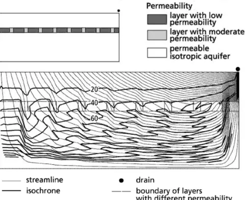
(9) 2.1.2 Variation in groundwater ages On a regional scale, the parameters that control this relationship may vary. For instance, the aquifer thickness is known to be less in the western part of the Dutch Meuse basin (Meinardi, 1994). Heterogeneity in the subsurface will also cause deviations from the ideal theoretical case, as can be seen in Figure 2.2. In this theoretical example, a discontinuous layer with low permeability affects the flow-field such that younger water is able to infiltrate locally to greater depths, replacing older water.. Figure 2.2: Effect of a discontinuous layer with low permeability on the flow field and age distribution. (After Broers and Van der Grift, 2004). These variations in groundwater age distribution will cause erroneous interpretation of the groundwater quality time series if the ideal theoretical relationship is assumed. Figure 2.3 shows the groundwater ages, as determined by 3H/3He groundwater dating (as presented in Deliverable T2.3) plotted against the groundwater ages predicted by equation 2.1, to show the variation in groundwater ages.. Deliverable T2.4, final draft, December 1st. 6.

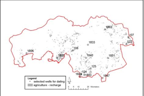
(10) Figure 2.3: 3H/3He ages plotted against the expected theoretical ages.. 2.2. Data. The data used for the profiles mentioned in the title were described Table 2.2 of Deliverable T2.1. Summarizing, the data include time series since 1980 or 1991 of the chemical composition of the groundwater sampled at 14 locations in agricultural recharge areas in the lower Meuse basin (shown on Figure 2.4). Measurements include field parameters (pH, EC and dissolved oxygen) concentrations of major cations (Na, K, Ca, Mg, Fe, Al and NH4) and anions (Cl, NO3, SO4, HCO3 and PO4) and trace metals (i.e. Cd, Cu, Ni, Zn). These data were readily avaiblable from the provincial monitoring network. For the present study, thirty-one screens between 4 and 26 m below surface level were sampled for tritium-helium. Samples were analyzed by the Institut für Umweltphysik of the Bremen University (Sültenfuß et al., 2004). The measurements were interpreted with an estimated recharge temperature of 10°C, an elevation of 0 m above sea level and a salinity of zero. See for further details deliverable T2.3. Tritium-helium ages were preferred over CFC and SF6 ages, because they were considered more reliable. This relates to the associated dissolved noble gas measurements which gave indications of age uncertainties.. Deliverable T2.4, final draft, December 1st. 7.

(11) Figure 2.4: Well locations in the agricultural recharge areas in the lower Meuse basin, listed in Table 2.2 of Deliverable T2.1. Chemical indicators The results of this procedure will be presented for six chemical indicators: three reactive targeted contaminants (nitrate, aluminum and potassium), and three conditionally conservative indicators (oxidation capacity (OXC), the chloride concentration and the sum of cations (SUMCAT)). These three chemical indicators are used because they are insensitive to specific subsurface reactions. The oxidation capacity was defined as the weighted sum of molar concentrations of NO3 and SO4 after Postma et al. (1991): OXC = 5 ∗ [NO 3− ] + 7 ∗ [SO 24 − ] OXC behaves conservatively during the process of nitrate reduction by pyrite oxidation under the condition that no other reactions occur, i.e. no subsurface denitrification by organic matter. Chloride is a conservatively transported ion under normal pH conditions. The sum of cations (in fact, major cations: Na, K, Mg, Ca, Fe, Al, NH4) is useful as a conditionally conservative indicator when cation-exchange processes dominate the transport of the cations and mineral dissolution does not occur. Moreover, the sum of cations is an indicator of the total load of solutes in the groundwater.. 2.3. Back-scaling of time series. 2.3.1 Method Better knowledge of the age distribution among the wells enables the use of an alternative trend approach, which is based on “back-scaling” the time series with the known groundwater age. The main assumption is that groundwater age at a certain monitoring screen is constant in time (for example Goode, 1996) This assumption seems reasonable given the long time scales of transport compared with the time scales of seasonal transient effects. The individual time series which cover the monitoring period 1992–2004 were scaled back in time using the tritium-helium age. For example, the time series of a monitoring screen with an age of 9 years is scaled back to the period 1983–1995. 2.3.2 Example: Oxidation capacity Figure 2.5 shows the back-scaled time series of the oxidation capacity are presented. Each individual time series is assigned a unique color to distinguish between the time series. The time series now reflect the approximate recharge period. The advantages Deliverable T2.4, final draft, December 1st. 8.

(12) of the method are 2-fold: (a) every time series provides information over a range of recharge years, and (b) data of multiple time series is available for each recharge year. A LOWESS smooth (LOcally WEighted Scatter-plot Smoothing, Cleveland & Devlin, 1988) was used to generate a trend line through all the time series data in the graph. This trend line reflects the local median of all measurements, which in fact reflects the area aggregated median trend. This enables the direct comparison of the measured concentrations with the regional historical inputs, which were described in deliverable T2.2. A LOWESS smooth through all the time series is plotted in black. This curve indicates the local median of all the time series. The LOWESS smooth is interpreted as the aggregated median trend for the agricultural recharge areas of Figure 2.4. The dashed black lines are the LOWESS smooths through the residuals between the back-scaled time series and the original LOWESS smooth. These indicate the local 25 and 75 percentile trend of all the time series. This indicates a confidence interval around the LOWESS smooth. We are confident that a certain trend is well described by the LOWESS smooth, if the confidence shows the same trend. Since each data point of the time series is plotted at the year of recharge, the median curve or LOWESS smooth should resemble the curve of the historical surplus input of the agricultural recharge areas which was derived in deliverable T2.2 (red line).. Deliverable T2.4, final draft, December 1st. 9.

(13) Figure 2.5: Time series of oxidation capacity back-scaled to the year of recharge of the samples. A LOWESS smooth (black line) is used to show the overall trend in these data. Dashed black lines indicate the 50% confidence interval around the LOWESS smooth. Red line indicates expected values based on historical inputs. Individual time series from selected piezometers have unique colors.. A few remarks can be made about this plot. First of all, there is a large noise in the individual time series. From individual time series it is hard to distinguish a trend in oxidation capacity. However, combining all the measured data into an aggregated trend using the LOWESS smooth, a clear trend reversal is demonstrated for OXC with a peak concentration around the year 1985. Both the LOWESS smooth itself, as the 25 and 75 percentile smooths increase towards a maximum observed oxidation capacity in groundwater that has recharged in 1985. Younger water shows a downward trend, resulting from the establishment of the Manure Law in 1985 and reduction of manure inputs from that time onward. 2.3.3 Results From the study of the historical inputs, as described in Deliverable T2.2, we expect an upward trend in the concentrations in water recharging before 1985, and a downward trend in groundwater recharging after 1985 for solutes that travel with the same velocity as the groundwater itself. The following figures of back-scaled time series of conservative chemical indicators (OXC, Cl- and SUMCAT) confirm these expectations. The reactive indicators (NO3-, Al and K+) show a somewhat different behaviour, as a result of subsurface reaction and consequently non-conservative transport.. Deliverable T2.4, final draft, December 1st. 10.

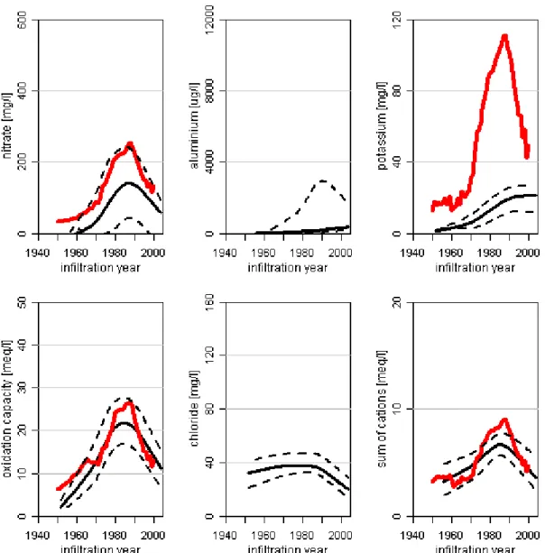
(14) Figure 2.6: Comparison of measured trends (LOWESS smooths through back-scaled time series of six chemical indicators, in black) with historical inputs (red). Reactive indicators (top) show large discrepancies with historical inputs. Conservative indicators (bottom) are consistent with the expected trends.. 2.3.4 Conservative indicators The LOWESS smooth in Figure 2.6 indicates an increasing trend over the period 1950–1985 for all conservative indicators (bottom), a trend reversal and decreasing trends after 1985. There is a striking similarity between the estimated historical inputs and the trend derived from the monitoring data, even though the individual time series showed large fluctuations and probable measurement errors. This confirms the expectation that OXC and the sum of cations behave conservatively in the subsurface and confirms the increase of concentrations until the introduction of the Netherlands Manure Law in 1985 and the decrease afterwards. 2.3.4 Reactive chemical constituents The discrepancy between the expected and actual concentrations of nitrate (top left) are probably caused by denitrification by pyrite oxidation or organic matter in the saturated zone. Nitrate concentrations are lower than expected when nitrate would have been transported conservatively. The 25 percentile trend even indicates that 25% of the agricultural areas have concentrations below 50 mg/l for all infiltration years. However, the median aggregated nitrate trend clearly shows trend reversal with a peak. Deliverable T2.4, final draft, December 1st. 11.

(15) around 1985. Given the close resemblance between the OXC measured and expected trends, we propose that the main mechanism of nitrate removal is the oxidation of pyrite. Earlier studies indeed show the presence of abundant pyrite in the NoordBrabant subsoil (for example Broers 2004). Aluminum shows strong adsorption and retardation. The upper confidence limit of the LOWESS smooth does indicate the expected trends, but the median aggregated LOWESS smooth is still increasing in the low concentration range. This is attributed to the slow vertical movement of the acidification front. Similarly, the potassium concentrations are increasing slowly in younger groundwater, unlike the input curve. Although the input curve is sharply decreasing since 1985, the aggregated median trend mooth is increasing slowly into the 1990s. The concentrations remains constant in younger waters, but no trend reversal can be observed. This is attributed to the retarding effect of cation exchange between potassium and calcium and magnesium; the ratio between the slopes of the input curve and the actual measured trend slope give some indication on the effective retardation factor, which is about three. This would mean that the maximum concentrations might only be reached after the year 2020. 2.3.5 Conclusions A groundwater dating method such as 3H/3He provides a novel tool to detect trend reversal, aggregating monitoring data for larger areas. This removes the uncertainty in trend analysis that is caused by groundwater age variations. Large year to year variation in concentrations remain, but the back-scaling of time series yields a large number of data points for each year of infiltration. Trends are readily observed in backscaled time series. The observed trend reversal in the aggregated monitoring data could well be related to the pattern of historical inputs. The upward trend in concentrations up to 1985 is clear in all conservative indicators. Even better visible is the trend reversal and subsequent downward trend since 1985, caused by the establishment of the Manure Law and the subsequent reduction of manure inputs. Overall, the described novel approach for detection of trend reversal is well suited to meet the objectives of the draft Groundwater Directive, as illustrated in Figure 1.1. The observed trend can well be related to the reconstructed historical inputs. This allows the trend propagation and extrapolation based on estimates of future land use, which will be presented in the following sections.. 2.4. Trend extrapolation. 2.4.1 Correlation of back-scaled time series with historical inputs To propagate the trends observed in the time series into the future, we rely on the extrapolation of the input curves and expected future land use. To do so, we need to know whether these input curves are reliable in hindsight. Correlating the historical inputs to the observed trends will yield such information. So before extrapolating the observed trends using land use scenarios, a simple linear regression between the input curves and the LOWESS smooths was applied. This was performed for oxidation capacity and sum of cations (being conservative indicators) and nitrate. Because of the non-conservative transport of the reactive indicators, this simple trend propagation is not valid for other indicators and would require modelling of the transport of these chemicals incorporating the subsurface reactions, which is beyond the scope of this document. Examples of such an approach were given in Broers & van der Grift (2004).. Deliverable T2.4, final draft, December 1st. 12.

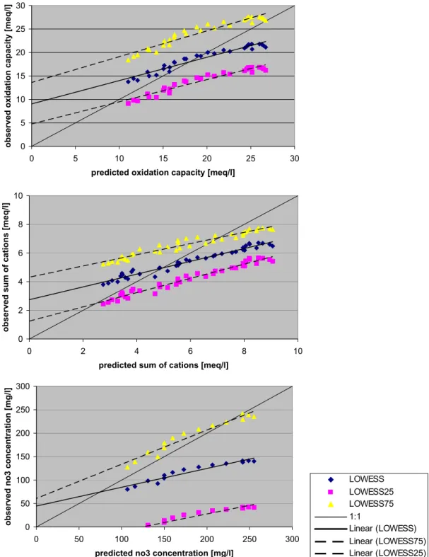
(16) observed oxidation capacity [meq/l]. The linear regression plots of the oxidation capacity and sum of cations are presented below. In each plot, the predicted concentrations are on the horizontal axis. On the vertical axis are the data points of the observed LOWESS smooth and data points of the LOWESS smooth indicating the 25 and 75 percentile. 30 25 20 15 10 5 0 0. 5. 10. 15. 20. 25. 30. predicted oxidation capacity [meq/l]. observed sum of cations [meq/l]. 10 8 6 4 2 0 0. 2. 4. 6. 8. 10. observed no3 concentration [mg/l]. predicted sum of cations [meq/l] 300 250 200 150 100 50 0 0. 50. 100. 150. 200. 250. 300. predicted no3 concentration [mg/l]. LOWESS LOWESS25 LOWESS75 1:1 Linear (LOWESS) Linear (LOWESS75) Linear (LOWESS25). Figure 2.7: Linear regression between the predicted oxidation capacity (a), sum of cations (b) and nitrate concentration (c) from historical inputs and the LOWESS smooth through the observed data.. There is an excellent correlation between the historical inputs and the observed concentrations. The correlation coefficients for the LOWESS smooth are as high as 0.96, 0.98 and 0.94 for oxidation capacity, sum of cations and nitrate respectively. However, this relationship is not proportional. The prognosis seems to overestimate Deliverable T2.4, final draft, December 1st. 13.

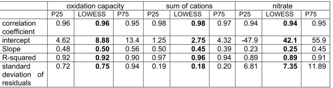
(17) high concentrations and underestimate lower concentrations. The result is a set of regression lines with a considerable intercept and a slope angle of less than 1. All parameters of the regression lines are presented in Table 2.1. Table 2.1: Regression statistics of predicted and observed oxidation capacity, sum of cations and nitrate. oxidation capacity sum of cations nitrate P25. correlation coefficient intercept Slope R-squared standard deviation of residuals. LOWESS. P75. P25. LOWESS. P75. P25. LOWESS. P75. 0.96. 0.96. 0.95. 0.98. 0.98. 0.97. 0.94. 0.94. 0.95. 4.62 0.48 0.92 0.72. 8.88 0.50 0.92 0.75. 13.4 0.56 0.90 0.94. 1.25 0.50 0.97 0.19. 2.75 0.45 0.96 0.18. 4.32 0.39 0.94 0.20. -47.9 0.23 0.89 6.81. 42.1 0.25 0.89 7.35. 55.9 0.45 0.91 11.89. Although there does not seem to be a 1:1 relationship between input and observed concentrations, we will use these regression lines to circumvene this. The residual error of the regression line has a standard deviation of 0.75 and 0.18 for oxidation capacity and sum of cations respectively. Under the assumption that the underlying processes do not change, we would be able to predict the LOWESS smooth of the oxidation capacity with a confidence interval of 1.5 meq/l on either side. Back-scaled time series give the opportunity to ‘validate’ the estimates of the historical inputs. Here we used a simple linear regression to relate the historical inputs to the actually observed values of oxidation capacity and sum of cations. This linear regression showed that there is a good correlation between the predictions based on historical input and the observed series. The relationship is not proportional, and large values are over predicted by the input function. The historical curve for oxidation capacity seems not to fit the observed curve well before 1970. The estimates for the atmospheric deposition of this period are quite uncertain. To obtain a better correlation, we have used only data on groundwater that has recharged after 1970. Especially since this regression line will be used to predict ahead future concentrations, the error introduced by the uncertainty in atmospheric deposition is unwanted. The historical curve for the sum of cations structurally overestimates the observed curve before 1960. This error seems to have propagated from the (over) estimated use of (calcium) fertilizer in this period. Again, to improve the regression line, we have only used data of the period 1960-present. The upward part of the trend of nitrate is affected by pyrite oxidation and denitrification in deeper and older water. This does not affect the downward part of the trend as much and therefore only recent (post 1985) groundwater data was used in the regression. 2.4.2 Future inputs of agricultural pollution A new system of regulating manure and fertilizer use will be in place in the Netherlands as of January 1st 2006. This scheme reduces the maximum allowable amount of nitrogen and phosphor that may be applied to agricultural land, with respect to the current legislation. The aim of the new system is to furhter comply with EU Nitrates Directive and specifically to reduce the concentration of nitrate in the upper five meter of groundwater to the required level of 50 mg/l. In the period 2006 to 2008, maximum allowed manure use is reduced gradually towards levels which are to comply with the 50 mg/l standard. Failure to reach this limit will result in further reduction of the inputs. Deliverable T2.4, final draft, December 1st. 14.

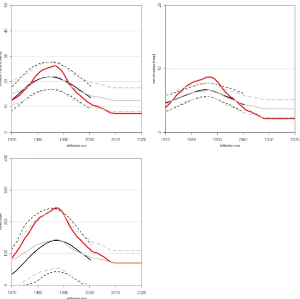
(18) Using the same accounting system of manure and fertilizer distribution as described in Deliverable T2.2, the effects of the measures on the deposition of other chemicals has been calculated. The following assumptions have been made to perform these calculations: • land use ratios remain constant • concentrations of chemicals in manure, fertilizer and crops remain constant • crop yield remains constant • atmospheric deposition remains constant Furthermore, we assume that the Netherlands will comply to the EU threshold in 2010, and that the 2010 regulations remain in effect in the following years. 2.4.3 Trend extrapolation Under these assumptions, the following input curves for nitrate, oxidation capacity and sum of cations are obtained. These were used to extrapolate the LOWESS smooth through the back-scaled time series graphs, as in Figure 2.8 .. Figure 2.8: Extrapolated time trends of oxidation capacity, sum of cations and nitrate concentration. Extrapolation (gray) uses linear regression between observed LOWESS smooth curves (black) and predicted concentrations (red).. Deliverable T2.4, final draft, December 1st. 15.

(19) The extrapolated time trend of oxidation capacity shows only a gradual decrease over the period 2000-2020. This extrapolated trend seems to be weaker than the one observed in the LOWESS smooth, but keep in mind that the most recent years of the LOWESS smooth are based on very few measurements. The extrapolated time trend of sum of cations seems more consistent with the observed trend of the LOWESS smooth. It shows a gradual decrease towards about 5.5 meq/l. The extrapolated median time trend of nitrate very slowly decreases towards about 80 mg/l in 2020. As with oxidation capacity, the predicted decrease seems to be weaker than the trend in the LOWESS smooth. Note that the concentrations still seems to stay above 100 mg/l in 25% the cases, based on the extrapolated P75 trend). These results derived from measured data indicate that the proposed manure reduction might not be enough to actually reach the standard of 50 mg/l in groundwater. Using the groundwater ages in the sampled wells, it is possible to predict the median concentrations of chemical indicators in groundwater that will be sampled during the next 10 or 20 years. So for each well, a median (and P25 and P75) prediction can be made for some time in the future. The median of these individual predictions will serve as the predicted concentration for the agriculture-recharge area. Individual time series may vary strongly from this median. This procedure has been applied to the shallow and deep screens separately, to gain insight in the changes in concentrations at different depth intervals.. deep. shallow. Table 2.2: Predicted median and maximum of regional averaged OXC, SUMCAT and NO3 concentrations at the shallow and deep screen level. OXC SUMCAT NO3 year Median Max Median Max Median Max (LOWESS) (P75) (LOWESS) (P75) (LOWESS) (P75) 2005 2010 2015 2030 year 2005 2010 2015 2030. 15.0 13.8 12.7 12.6. 27.2 28.0 24.2 18.0. 4.7 4.1 3.7 3.7. 7.5 7.7 7.0 5.3. 91.7 81.3 71.6 70.8. 220.5 239.0 198.6 115.1. 18.4 20.3 20.4 13.6. 28.0 27.8 28.0 22.0. 5.8 6.2 6.2 4.0. 7.7 7.7 7.7 6.5. 113.6 128.9 127.3 79.8. 239.0 237.3 239.0 170.4. It shows that improvements in groundwater quality at a certain depth will be very slow, largely because of the variation in groundwater ages. Median groundwater quality in shallow screens will slowly improve. Improvement of the maximum of the P75 prognosis will only occur in 25 years, because groundwater in all screens has than been recharged with low inputs groundwater. Before that time, some screens will still sample groundwater from around the nitrate peak. Groundwater quality in deep screens is expected to deteriorate in the near future – until the arrival of the 1985 manure peak – before improving. 2.4.4 Discussion Groundwater age dating has proven to be very helpful when researching trends in groundwater quality. Part of the variation in measured concentrations can be explained by variation in groundwater ages, and when this part is reduced, the trends resulting from changes in land use become more apparent. The trend reversal and subsequent downward trend have been observed in conservative chemical indicators (oxidation. Deliverable T2.4, final draft, December 1st. 16.

(20) capacity and sum of cations) and the downward trend can now also be observed in the concentrations of nitrate in young groundwater. With this concentration-recharge year relationship, the concentration time series can be extrapolated using a prediction of future land use. The correlation between the predicted concentrations and the measured concentrations was such that a reliable prediction for the future can be made. The largest source of uncertainty is in the estimates of manure and fertilizer use. These were based on the policy measures laid out for the period until 2010. Policy changes after evaluation of these measures may yield a stronger or a weaker downward trend in shallow groundwater quality. Using the groundwater ages and the extrapolated time trends to predict future groundwater quality shows that regional improvements of groundwater quality will be very slow because of the variation in groundwater ages. Monitoring screens from which relatively old water is sampled will produce polluted water for a longer period of time than screens with young water. These “older screens” cause the long waiting time before groundwater quality has improved over the whole region at a certain depth level.. Deliverable T2.4, final draft, December 1st. 17.

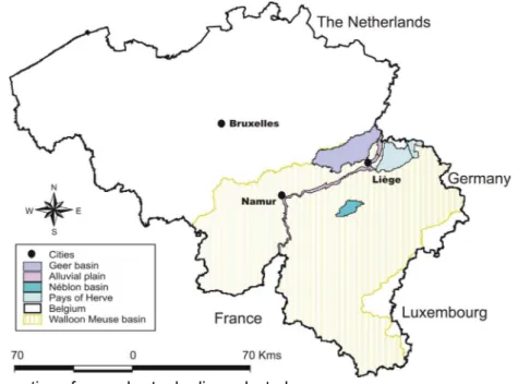
(21) 3. Point by Point Statistical Trend Analysis and Extrapoled Time Trends at Test Sites in the Meuse BE (ULg) J. Batlle Aguilar1, Ph. Orban1, S. Brouyère1,2 1 Group of Hydrogeology and Environmental Geology, HGULg 2 Aquapôle Ulg University of Liège, Building B52/3, 4000 Sart Tilman, Belgium Tel: +32.43.662377 Fax: +32.43.669520, Serge.Brouyere@ulg.ac.be. 3.1. Introduction. The Hydrogeology Group of University of Liège (HGULg) has selected 4 main groundwater bodies in the Walloon Meuse basin to study groundwater nitrate concentration trends: The Hesbaye groundwater body (Geer basin), the Pays of Herve groundwater body, the Néblon basin and the alluvial plain of the Meuse river (Figure 3.1). The present deliverable describes in detail the dataset of nitrate measurements (number of points, main features…) collected in these basins and the statistical trend analysis that has been performed on these data.. Figure 3.1. Location of groundwater bodies selected.. 3.2. Description of the dataset of nitrate measurements. 3.2.1 Update of the nitrate dataset Nitrate concentrations used in this study are mainly from the Nitrate Survey Network established by the Walloon Region Government. In this network, boreholes, springs, galleries and traditional wells, where sampling and water analyses are carried out regularly are considered as monitoring points. This network provides a spatial and. Deliverable T2.4, final draft, December 1st. 18.

(22) temporary representation of nitrate contents in the aquifers. Nevertheless, gaps exist in the datasets and in the spatial distribution of monitoring points. Annual data obtained from these analyses are stored in a database owned by the Walloon Region authorities. Up to now, the latest data available comes from the end of 2003. The 2004 dataset is still under compilation in the Walloon Region and it was not yet available at the time of preparing this deliverable During the last months, contacts have also been established with the VMW (Vlaamse Maatschappij voor Watervoorziening), the Flemish water supply company, in order to have access to data and to water supply wells in the North of the Hesbaye groundwater body (included in the Geer basin). In Flanders, the Hesbaye chalk aquifer is confined, in contrast to the unconfined part of the aquifer within Walloon Region territory. Some points has been deleted from table presented in Deliverable T2.1, because the number of records were clearly not enough to carry out a trend analysis, and new points from the VMW has been added for the Geer basin (denoted with the HF code in Table 1). Table 3.1, 3.2, 3.3 and 3.4 in Appendix 3.1 present an updated summary of data availability for nitrate trend analysis in groundwater bodies selected in the Walloon Meuse basin.. Deliverable T2.4, final draft, December 1st. 19.

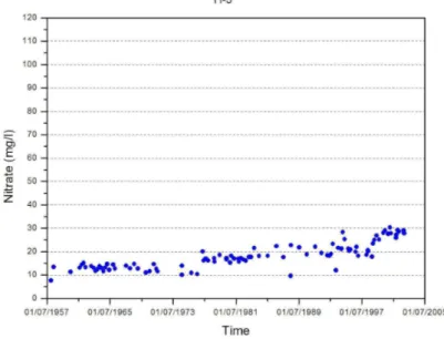
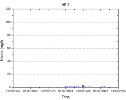
(23) 3.2.2 Dataset features Time-series graphs are presented for some sampling points to have a first idea of the main features of the datasets (seasonality, outliers…) and the presence of trends. Some interesting general features are pointed out here after. Spatial variations in nitrate contents in the Hesbaye aquifer Because of the geological context of the Hesbaye plateau, hydrogeological conditions prevailing in the chalk aquifer change from unconfined in the Southern part of the basin to confined conditions in the Northern part. As a direct consequence, nitrates are almost absent in groundwater of the North of the basin, while concentrations are close to the drinking limit in the South. Figure 3.2 and 3.3 shows characteristic time-series from the South and North part respectively. The absence of nitrate in the North may have two explanations: the occurrence of denitrification processes in the confined part of the aquifer or the occurrence of very old, still uncontaminated groundwater. This will be discussed later on.. Figure 3.2. Characteristic time-series from a point located in the Southern part of the Hesbaye aquifer.. Deliverable T2.4, final draft, December 1st. 20.

(24) Figure 3.3. Characteristic time-series of a point located in the Northern part of the Hesbaye aquifer.. Periodic (“seasonal”) variations in nitrate contents Many datasets coming from the Hesbaye and the Pays de Herve groundwater bodies exhibit clear periodic variations in nitrate concentrations (Figure 3.4 and 3.5). As discussed by Brouyère et al., (2004), such periodic variations are explained by groundwater table fluctuations in the variably saturated dual-porosity chalk. In principle, nitrate spread over the land surface progressively infiltrate across the unsaturated zone and migrate slowly downward through the unsaturated chalk matrix. Under low groundwater level conditions, the nitrate contamination front is disconnected from the aquifer and nitrate concentrations in the aquifer tend to diminish because of dispersion and mixing processes. When groundwater levels rise, the contamination front is quickly reached and leached: the contamination source is re-activated and nitrate concentrations are likely to increase rapidly in the saturated zone. This effect is observed in the Geer basin and in the Pays of Herve but not in the Néblon basin (mostly limestone aquifers) and in the alluvial plain aquifer (gravel aquifer).. Deliverable T2.4, final draft, December 1st. 21.

(25) Figure 3.4. Multi-annual variations in nitrate concentration at sampling point H-15 in the Geer basin.. Figure 3.5. Multi-annual variations in nitrate concentration at sampling point PH-7 in the Pays of Herve groundwater body.. In the Geer basin, a very dense network is available for monitoring variations in groundwater levels. As an illustration, Figure 3.6 shows groundwater table variations for the longest datasets available in the basin (from 1951 to 2003). Unfortunately, this network does not necessarily correspond to nitrate sampling locations.. Figure 3.6. Groundwater level measurements from 1951 to 2003.. Figure 3.7 and 3.8 show groundwater level and nitrate concentration time plots at neighbouring observation points. These examples confirm the major impact of periodic variations in groundwater levels on the dynamics of nitrate in the chalk aquifer. In the subsequent statistical analysis, the seasonal effect of such periodic variations has not. Deliverable T2.4, final draft, December 1st. 22.

(26) been accounted for explicitly because of the difficulty in defining the periodicity of such effects that are related to pluri-annual variations in precipitations. Neglecting the seasonality is not a problem in trend detection provided that the datasets integrate several periods so that the periodic variations compensate and the global trend emerges. Doing so on a reduced period of time could of course lead to wrong conclusions. In a shorter observation window, the general trend is less likely to be observed. As an example, performing a trend calculation on a sub-dataset corresponding to decreasing groundwater levels could probably lead to the conclusion of a decrease of nitrate concentrations in the aquifer with time. Reliability of results depends on the length of the time series: longer series will yield more reliable results. This is the case for datasets H-9 and H-11 (see Annex). Dataset H-9 provide nitrate data on a long period of time, while dataset H-11 is relatively short. For H-9, the result is “evidence of an upward trend”, while for H-11, there is “no evidence of a trend”. Such a difference in the result can be explained by the length of H-11, which does not allow one detect anything in the trend analysis. For the datasets in the Geer and Pays of Herve groundwater bodies, the analysis has been carried out having this potential problem in mind. However, most of the time, datasets that were too short were naturally “eliminated” at the trend detection level, the regression test or the Mann Kendall test, which is robust enough to conlude that no trend is present.. Figure 3.7. Time series of nitrate concentration (point H-15) and groundwater level measurements (point 750).. Deliverable T2.4, final draft, December 1st. 23.

(27) Figure 3.8. Time series of nitrate concentration (point H-13) and groundwater level measurements (points 17 and 730).. Presentation of the nitrate datasets A total of 97 time-series is presented for the four selected groundwater bodies in Appendix 3. The same time and concentration scales are used for each dataset of a given groundwater body to allow visual comparison of data from one point to another. Figure 3.9 shows an example of a nitrate time plot for each of the four selected groundwater bodies considered in the Walloon part of the Meuse basin.. Deliverable T2.4, final draft, December 1st. 24.

(28) Figure 3.9. Nitrate concentration time-series for the Geer basin (top left), Pays of Herve (top right), Néblon basin (bottom left) and the alluvial plain aquifer (bottom right).. 3.3. Statistical trend analysis. 3.3.1 Methodology For the trend analyses of groundwater quality data in the Walloon region, the following procedure has been used (Figure 3.10):. DATASET Shapiro-Wilks test (<50 values) Shapiro-Francia test (>50 values). 1). 2). Normality. Non-Normality. Linear regression. Mann-Kendall test. Trend. 3). No trend. Slope regression. Trend. No trend. Kendall's Slope. Figure 3.10. A three step procedure is adopted for trend analysis of nitrate concentrations in the selected groundwater bodies: 1) normality test; 2) trend detection; 3) trend estimation.. (1) Normality of the dataset The first step is to evaluate whether the dataset is normally distributed or not. If the number of records is less than 50, the Shapiro-Wilks test is used. If the number of records is equal or larger than 50, the Shapiro-Francia test is used. D’Agostino’s test has been also used to corroborate the results obtained using the two other techniques. For most datasets, the D’Agostino’s test corroborates the result obtained with one of the two other tests. For the datasets for which the results of the normality test are contradictory, it has been decided to apply both trend detection techniques. The choice of trend detection method is a function of the results obtained in this step: parametric tests are performed on normally distributed datasets and non-parametric tests are performed on non-normally distributed datasets. (2) Trend detection The second step consists in performing a test aiming at detecting whether a trend exists or not in the dataset. For normally distributed datasets, linear regression is applied. The correlation coefficient r is used as an indicator of the existence of the trend. In accordance with (Carr 1995), three ranges of correlation degree (trend robustness) have been considered for the correlation between time and nitrate concentrations: • • • •. strong correlation for r values ranging between 0..8 and 1 (or -0.8 and -1); moderate correlation for r values ranging between 0..5 and 0..8 (or -0.5 and -0.8); weak correlation for r values ranging between 0.1 and 0.5 (or -0.1 and -0.5); no correlation for r values ranging between -0.1 and 0.1.. Deliverable T2.4, final draft, December 1st. 25.

(29) For trend detection on non-normally distributed datasets, the non-parametric MannKendall test has been selected. It has to be mentioned that this test is very appropriate for groundwater quality data, when the amount of records is often limited and the data distribution usually not known. It has been applied previously with reliable results in numerous studies, including hydrological applications (Hirsch et al., 1982; Lettenmaier et al., 1991; Loftis et al., 1991; Zetterqvist 1991; Smith and McCann 2000; Hanson 2002; Libiseller and Grimvall 2002; Schnabel 2002; Yue et al., 2002; Robinson et al., 2003; Zhang and Zwiers 2004). The Mann-Kendall test determines the existence of a trend by the calculation of an index reflecting the frequency with which concentrations observed in later samples are greater or less than those observed in earlier samples. It is based on the calculation of differences between pairs of successive data. For deciding if a trend exists in the Mann-Kendall test, a significance level of 99% has been considered, corresponding to a threshold value of 2.32634 for the Mann-Kendall index. (3) Trend estimation The third step in the trend analysis is the trend estimation or quantification. For normally distributed datasets, the trend magnitude is defined by the slope of the linear regression equation. For non-normally distributed datasets, the trend magnitude is based on the calculation of the Sen’s slope, by calculating the median of all data pairs in dataset (Hirsch et al., 1991). Is less affected by data errors, outliers or missing data than the linear regression (Hanson 2002). 3.3.2 Results from trend analysis on individual time series Table 3.1 summarizes the results of trend analysis grouped by groundwater bodies. Estimations of slopes values are given in mg per year. Detailed results are presented in Tables 3.2 to 3.5. Groundwater body. Number of nitrate points. Number of Number of downward upward trends trends 26 0 15 Geer basin 12 2 6 Pays of Herve 6 1 4 Néblon basin 38 15 11 Alluvial plain Table 3.1. Summary of trend tests results for each groundwater body. Percent of significant trends 57.7% 66.6% 83.3% 68.4%. Table 3.5 shows the number of significant trends (both upward and downward) at the nitrate points where statistical test was carried out. One can observe, except for the Néblon sub-basin, that in about 60% of the time series a significant trends is present. For the Néblon sub-basin just 6 points were taken into account, which could explain the high percentage of significant trends.. Deliverable T2.4, final draft, December 1st. 26.

(30) Non-norm.. H-5. Non-norm.. Non-norm.. Non-norm.. H-8. H-9. H-10. Non-norm.. Non-norm.. H-18. H-19. Non-norm.. Non-norm.. H-15. H-17. Non-norm.. H-14. Normality. Non-norm.. H-13. H-16. Non-norm.. H-12. H-11. Normality. H-7. Non-norm.. Non-norm.. H-4. Non-norm.. Non-norm.. H-3. H-6. Non-norm.. H-2. Sh.-Francia test. Non-norm.. Sh.-Wilks test. H-1. Code. Normality test. 0.1442. 0. 0.5292. 0.8881. 0.8405. 0.3791. r. Strong. Strong. Weak. ---. ---. ---. Weak. Null. Moderate. ---. ---. ---. ---. ---. ---. ---. ---. ---. ---. Correlation. 2.07958. 7.15834. 2.22759. 0. -0.49318. 4.42336. 3.82585. 5.50093. -2.14892. 7.69519. 4.96828. 5.54954. 8.93565. 1.31197. 2.78247. 0.43333. 9.94543. 3.92641. No trend. Upward. No trend. No trend. No trend. Upward. Upward. Upward. No trend. Upward. Upward. Upward. Upward. No trend. No trend. No trend. Upward. Upward. Mann-Kendall Comparison Trend level 8.63554 Upward. Deliverable T2.4, final draft, December 1st. Normality. Non-norm.. Non-norm.. Normality. Non-norm.. Normality. Non-norm.. Non-norm.. Non-norm.. Non-norm.. Non-norm.. Non-norm.. Normality. Non-norm.. Non-norm.. Non-norm.. Normality. Normality. Non-norm.. D’Agostino’s test. Linear Regression. Trend detection. 0.146. ---. ---. 0. ---. 0.4745. ---. ---. ---. ---. ---. ---. 0.584. ---. ---. ---. 0.3285. 0.2555. ---. Linear Slope. ---. 0.4803. ---. ---. ---. 0.4525. 0.3075. 0.3249. ---. 0.3868. 0.0928. 0.5408. 0.5883. ---. ---. 0.3647. 0.2450. 0.4756. Sen’s slope. Trend estimation (mg/y). ▲ ▲ ▲ ● ● ● ▲ ▲ ▲ ▲ ● ▲ ▲ ▲ ● ● ● ▲ ●. Trend analyse result. 27.

(31) Non-norm.. Non-norm.. HF-21. Normality. HF-19. Normality. Non-norm.. 0.6905. 0.4277. 0.0954. 0.6875. 0.3632. r. ---. Moderate. Weak. 0. Weak No nitrate No nitrate No nitrate No nitrate No nitrate No nitrate No nitrate No nitrate No nitrate No nitrate No nitrate No nitrate No nitrate No nitrate No nitrate No nitrate Moderate. Correlation. Linear Regression. 1.58516. 11.6486. 0. 11.436 ---. No trend. Upward. No trend. Upward. Mann-Kendall Comparison Trend level 3.68364 Upward. Trend detection. Deliverable T2.4, final draft, December 1st. Non-norm.. Normality. Non-norm.. Normality. Normality. D’Agostino’s test. Normality. Sh.-Francia test. HF-20. Normality. Sh.-Wilks test. HF-18. H-20 HF-1 HF-2 HF-3 HF-4 HF-5 HF-6 HF-7 HF-8 HF-9 HF-10 HF-11 HF-12 HF-13 HF-14 HF-15 HF-16 HF-17. Code. Normality test. ---. 0.803. -0.9125. -0.073. 0.7665. 7.7745. Linear Slope. ---. 0.8004. ---. 0.8058. 1.6489. Sen’s slope. Trend estimation (mg/y). ▲ ● ● ▲ ●. ▲. Trend analyse result. 28.

(32) Trend detection. Trend estimation (mg/y). Code. Deliverable T2.4, final draft, December 1st. Linear Regression. Trend analyse Mann-Kendall Sh.-Wilks Sh.-Francia D’Agostino’s Linear Sen’s result Comparison test test test Slope slope Correlation Trend r level HF-22 Non-norm. Non-norm. --10.3717 Upward --0.3266 ▲ Table 3.2. Point-by-point trend results for the Geer basin (▲ evidence of upward trend; ▼ evidence of downward trend; ● no evidence of trend).. Normality test. 29.

(33) Normality. Normality. PH-5. PH-6. Normality. PH-10. Normality. Normality. Non-norm.. Normality. Non-norm.. Non-norm.. Normality. Normality. Normality. Normality. D’Agostino’s test. 0.4401. 0.8848. 0.3391. 0.0721. 0.8433. 0.4243. 0.2629. 0.7281. 0.6022. r. --Weak. Strong. Weak. 0. Strong. Weak. Weak. Moderate. Moderate. Correlation. Linear Regression. 2.3416. ---. 0.0702. 5.7037. ---. ---. 2.6965. -0.9826. 3.1244. Upward. ---. No trend. Upward. ---. ---. Upward. No trend. Upward. Mann-Kendall Comparison Trend level -----. Trend detection. 0.3285. 5.4750. ---. 0.5475. 0.0365. 0.4745. 0.4380. -0.2555. 1.6060. -4.3800. Linear Slope. 0.3166. ---. ---. 0.7335. ---. ---. 0.5320. ---. 1.7528. ---. Sen’s slope. Trend estimation (mg/y). ▼ ▲ ● ▲ ▲ ● ▲ ● ▲ ▲ ▼. Trend analyse results. Deliverable T2.4, final draft, December 1st. 30. PH-11 Non-norm. Non-norm. ---2.7072 Downward ---0.3760 Table 3.3. Point-by-point trend results for the Pays of Herve groundwater body (▲ evidence of upward trend; ▼ evidence of downward trend; ● no evidence of trend).. Normality. PH-9. Non-norm.. Normality. PH-4. PH-8. Normality. PH-3. Normality. Non-norm.. PH-2. Sh.-Francia test. PH-7. Normality. Sh.-Wilks test. PH-1. Code. Normality test.

(34) Non-norm.. Non-norm.. Non-norm.. N-3. N-4. N-5. Non-norm.. Non-norm.. Non-norm.. Normality. Normality. D’Agostino’s test. 0.8281. 0.6210. r. ---. ---. ---. Strong. Moderate. Correlation. Linear Regression. 11.1355. 8.77369. 10.7388. 11.2545. Upward. Upward. Upward. Upward. Mann-Kendall Comparison Trend level -3.31628 Downward. Trend detection. ---. ---. ---. 0.5840. -0.8395. Linear Slope. 0.2536. 0.1677. 0.1929. 0.6881. -0.8773. Sen’s slope. Trend estimation (mg/y). Deliverable T2.4, final draft, December 1st. ▼ ▲ ▲ ▲ ▲ ●. Trend analyse result. N-6 Normality Normality 0.1153 Weak -0.334242 No trend 0.0730 --Table 3.4. Point-by-point trend results for the Néblon basin (▲ evidence of upward trend; ▼ evidence of downward trend; ● no evidence of trend).. Normality. Normality. N-1. Sh.-Francia test. N-2. Sh.Wilks test. Code. Normality test. 31.

(35) Normality. Normality. Normality. Non-norm.. Non-norm.. Normality. Non-norm.. Normality. Normality. AP-11. AP-12. AP-13. AP-14. AP-15. AP-16. AP-17. AP-18. Normality. AP-7. AP-10. Normality. AP-6. Non-norm.. Non-norm.. AP-5. AP-9. Normality. AP-4. Normality. Non-norm.. AP-3. AP-8. Normality. AP-2. Sh.-Francia test. Non-norm.. Sh.-Wilks test. AP-1. Code. Normality test. 0.6709. 0.5128. 0.6127. 0.1407. 0.4518. 0.1217. 0.4695. 0.6068. 0.2383. 0. 0.7408. 0.3886. 0.2569. r. Weak. Weak. Weak. Weak. Weak. Weak. Moderate. Moderate. Moderate. ---. ---. ---. Moderate. Weak. 0. Moderate. ---. ---. Correlation. 3.2337. -1.7127. -4.6418. ---. -0.3409. 1.5310. -2.2111. 1.0722. 2.7363. -0.6719. -5.9796. -2.2253. -0.5452. 6.5608. 2.4662. 0.1322. -1.3817. Upward. No trend. Downward. ---. No trend. No trend. No trend. No trend. Upward. No trend. Downward. No trend. No trend. Upward. Upward. No trend. No trend. Mann-Kendall Comparison Trend level 0.8895 No trend. Deliverable T2.4, final draft, December 1st. Normality. Normality. Normality. Normality. Non-norm.. Non-norm.. Normality. Normality. Normality. Non-norm.. Normality. Normality. Normality. Normality. Normality. Non-norm.. Normality. Non-norm.. D’Agostino’s test. Linear Regression. Trend detection. 0.8760. -2.2995. -2.2630. 0.2555. ---. ---. -6.1320. 0.2920. 0.5840. ---. -2.1170. -0.2555. 0. 0.5475. 0.1825. ---. -0.4380. ---. Linear Slope. 0.7964. ---. -5.2647. ---. ---. ---. ---. ---. 0.6461. ---. -2.5489. ---. --. 0.5714. 0.1497. ---. ---. ---. Sen’s slope. Trend estimation (mg/y). ● ▼ ● ▲ ▲ ● ▼ ▼ ● ▲ ● ▼ ● ● ● ▼ ▼ ▲. Trend analyse result. 32.

(36) Non-norm.. AP-35. Normality. AP-31. Normality. Normality. AP-30. AP-34. Normality. AP-29. Normality. Normality. AP-28. AP-33. Non-norm.. AP-27. Non-norm.. Non-norm.. AP-26. AP-32. Normality. AP-25. Non-norm.. AP-23. Normality. Normality. AP-22. Normality. Sh.-Francia test. AP-24. Non-norm.. Normality. Sh.-Wilks test. AP-21. AP-20. AP-19. Code. Normality test. 0.4939. 0.5867. 0.1562. 0.1497. 0.2263. 0.4310. 0.5545. 0.2032. 0. 0.3297. 0.2573. 0.4309. r. Weak. 0. Weak. Weak. Weak. Weak. Weak. ---. Moderate. Moderate. ---. ---. ---. Moderate. ---. Weak. Weak. Correlation. 0.4333. -1.2368. ---. -4.4726. -3.3449. -3.5609. 1.0288. 2.8865. 4.8967. -0.1017. 5.2465. 1.5057. -1.0072. 1.6274. -2.8890. 0.8073. No trend. No trend. ---. Downward. Downward. Downward. No trend. Upward. Upward. No trend. Upward. No trend. No trend. No trend. Downward. No trend. Mann-Kendall Comparison Trend level 2.4539 Upward. Deliverable T2.4, final draft, December 1st. Non-norm. Normality. Normality. Non-norm.. Normality. Normality. Normality. Normality. Non-norm.. Non-norm. Normality. Normality. Normality. Normality. Non-norm.. Normality. Normality. D’Agostino’s test. Linear Regression. Trend detection. ---. -1.7520. -2.0440. ---. -0.2920. -0.2555. 0.4745. 0.6570. ---. ---. 1.0220. 0.4015. 0. 0.8395. ---. 0.5840. 0.5475. Linear Slope. ---. ---. ---. -6.2159. -0.5367. -0.7343. ---. 0.5713. 0.3896. ---. 1.3371. ---. ---. ---. -0.2276. ---. 0.5548. Sen’s slope. Trend estimation (mg/y). ▲ ▼ ▼ ▲ ● ▲ ▲ ● ▲ ▲ ▲ ▼ ▼ ▼ ▼ ▼ ●. Trend analyse result. 33.

(37) Normality. AP-37. Sh.-Francia test. Normality. Non-norm.. D’Agostino’s test. 0,8123. r --Strong. Correlation. Linear Regression. ---. ---. Mann-Kendall Comparison Trend level -4,1748 Downward. Trend detection. -7,5190. ---. Linear Slope. ---. -1,9967. Sen’s slope. Trend estimation (mg/y). ▼ ▼ ▼. Trend analyse result. Deliverable T2.4, final draft, December 1st. 34. AP-38 Non-norm. Normality 0,3106 Weak -3,4551 Downward -0,4745 -0,6294 Table 3.5. Point-by-point trend results for the alluvial plain groundwater body (▲ evidence of upward trend; ▼ evidence of downward trend; ● no evidence of trend).. Non-norm.. Sh.-Wilks test. AP-36. Code. Normality test.

(38) 3.3.3 Spatial trend distribution In order to have an overview of the spatial trend distribution, trend analysis results are represented in Figure 3.11 to 3.14. Figure 3.11 shows the distribution of nitrate trends in the Geer basin. As expected, a general upward trend is observed in the entire basin. However, as mentioned in point 2.2, two zones can be differentiated: the Southern part, corresponding to the unconfined part of the chalk aquifer, where high concentrations of nitrate are encountered, and the Northern part corresponding to the confined part of the chalk aquifer, where nitrate has not been detected (or at very low concentrations only).. Figure 3.11. Spatial trend distribution in the Geer basin.. Figure 3.12 shows the distribution in nitrate trends in the Pays de Herve groundwater body. The monitoring network is not as developed as in the Geer basin, however, a upward trend is generally observed. In these two groundwater bodies (Geer and Herve), it is logical to obtain similar results because of the same geology (fissured dual porosity chalk overlain by loess formations) and land use practices (intensive agriculture and farming).. Figure 3.12. Spatial trend distribution in the Pays of Herve groundwater body.. Deliverable T2.4, final draft, December 1st. 35.

(39) Figure 3.13 presents the distribution of nitrate trends in the Néblon basin. The sampling network is very limited but among these points, 4 of them are very integrative because they correspond to major drainage galleries owned by a water distribution company. These 4 points are characterized by upward nitrate trends. This confirms that the groundwater body is at risk, even if the nitrate pressure is less pronounced in that basin.. Figure 3.13. Spatial trend distribution in the Néblon basin.. Figure 3.14 presents the trend tests results for the alluvial plain. Most sampling locations do not exhibit trend or even downward trends in nitrates. In the alluvial plain however, land use mainly consists in urbanized and industrialized areas. Agriculture does not constitute a major source of contamination risk there. Furthermore, it is likely that the groundwater quality in the alluvial plain is strongly influenced by the interactions with the Meuse River. Groundwater – surface water interactions are influenced by the existence of dams regulating the level of water in the Meuse for navigation and by water supply wells in the alluvial aquifer. It could probably be interesting to consider these elements in a more detailed analysis of the results.. Figure 3.14. Spatial trend distribution in the alluvial plain groundwater body.. Deliverable T2.4, final draft, December 1st. 36.

(40) 3.4. General conclusions and perspectives. 3.4.1 Statistical trend analysis In this deliverable, a consistent and rigorous approach has been proposed and applied for trend detection and quantification in groundwater quality (nitrate) datasets, based on statistical techniques. Some general observations can be drawn from the point-by-point results obtained for the four groundwater bodies selected in the Walloon part of the Meuse basin. The statistical approach seems robust and able to discriminate between “clear” and “weak” trends. This is related to the two-step procedure: first trend detection, then trend quantification. For some datasets, the conclusions of the normality tests were not univocal. However, whatever the trend detection and quantification method applied to these datasets, conclusions were very similar. Even if, from a pure statistical point of view, the normality of the dataset is a factor to be considered for selecting one or another trend analysis technique, from a practical point of view, the result of the analysis is not so sensitive to the distribution of the dataset. 3.4.2 Extrapolating trends The statistical analysis has provided point-by-point estimations of nitrate trends, in the form of a slope expressed in mg NO3/year (increase or decrease). This result might be enough and appropriate to estimate the short term evolution of groundwater quality in the selected basins (few years), particularly for those groundwater bodies overlain by a thick unsaturated zone that lead to important buffer effects in the evolution of nitrate concentrations in the aquifers (Geer basin, Pays de Herve). However, end-users and decision makers such as water companies and regional authorities are more interested in the long term evolution of groundwater quality (tens of years) and geological and hydrogeological factors are not the only drivers of nitrate trends in groundwater: land use is also a key factor. The major disadvantage of using a “pure” statistical trend analysis is thus that it is not able to consider variations in land use and functional relations between land use and groundwater quality. For long term evaluation of nitrate trends, more advanced techniques are thus required, such as transfer functions or mechanistic modelling relating land use and groundwater quality. From a spatial point of view, advances are also still needed in order to produce reliable global estimates of groundwater quality indicators at the scale of the groundwater body, as requested by the EU Water Directive. 3.4.3 Future work Future work of HGULg in TREND T2 will be focused on the Geer basin where the nitrate dataset is dense and relatively uniformly distributed in the basin. Furthermore, this basin has been the topic of many previous geological and hydrogeological investigations, making it a very interesting case study for integrated research such as within AQUATERRA. Between March and May 2005, a sampling campaign was organized in the Geer basin (both in the Walloon part and in the Flemish region) for nitrate and tritium measurements. Water samples were sent to Dr P. Maloszewski and Dr. W. Stichler at GSF Münich for tritium analysis. It is expected that such measurements will contribute to a better understanding of spatial variations of nitrate concentrations in the chalk aquifer. Particularly, these results will contribute to explaining the absence of nitrate in confined part of the aquifer. Results have been obtained recently but time was too short to process them for this deliverable. A second sampling campaign is planned in the future. In the scope of BASIN R3 (Meuse) research activities, HGULg will develop a groundwater flow and transport model for the Geer basin in cooperation with COMPUTE C2. This model will be used in the scope of collaboration with workpackages HYDRO H1 (assessment of the impact of climate change on groundwater resources) and for nitrate trend analysis and forecasting in TREND T2.. Deliverable T2.4, final draft, December 1st. 37.

(41) For this purpose, it will also be investigated how nitrate trend results obtained in the Geer basin (presented in this deliverable) can be aggregated and used as calibration and validation datasets for the groundwater flow and transport model.. 3.5. Appendix. The 97 time-plots are included in the Appendix. These graphs correspond to 97 nitrate sites selected for the four groundwater bodies.. Deliverable T2.4, final draft, December 1st. 38.

(42) 4. Conventional and innovative approaches to trends analysis: a case study for the Brévilles catchment (BRGM) Pinault J.-L., Guyonnet D., Dubus I.G., Baran N., Gutierrez A. & Mouvet C BRGM BRGM Avenue C. Guillemin BP 6009 45060 Orléans Cedex 2 France T: +33 (0)2 38 64 47 50 F: +33 (0)2 38 64 34 46 i.dubus@brgm.fr. 4.1. Introduction. Crop protection products are known to represent a potential risk for human and the environment and the presence of pesticides is therefore routinely monitored in environmental media such as groundwater, surface water, and, to a lesser extent, the atmosphere. Surveillance programs for pesticides have different objectives. While some monitoring networks are specifically designed to ascertain whether there is any excess of legal threshold concentrations, most surveillance efforts are targeted towards investigating the spatial spread of the contamination of water resources by pesticides and/or detecting any positive or negative temporal tendency in concentrations. Designing a monitoring study to investigate trends in pesticide concentrations represents a significant investment given i) the costs involved in analysing organic compounds with accuracy; and, ii) the fact that the fate of pesticides is heavily influenced by weather conditions, which means that concentrations need to be monitored over a number of years sufficient to differentiate between variations due to climatic variability and those that can be attributed to measures taken to reduce pesticide contamination. The major contributing factors to the explanation of temporal variations in pesticide concentrations at a given groundwater point are likely to be: i) variations in transport properties (essentially governed by the effective rainfall, i.e. the part of the rainfall that effectively contributes to groundwater recharge); ii) spatial and temporal variations in annual applications of the pesticides; and, iii) possible variations in the potential for pesticide degradation. The limited number of factors involved and the strong influence of hydrology in the determination of pesticide trends in groundwater means that statistically-based approaches establishing a direct relationship between pesticide concentrations and water inputs to groundwater systems, such as transfer function, Bayesian-based or neural-network-based approaches are well suited to the reconstruction or prediction of past or future changes in groundwater concentrations. In contrast to more deterministic approaches, data requirements are generally low, ensuring their cost effectiveness. The present document reports on the comparative application of three different approaches to trends analysis for concentrations of pesticides in water resources. A total of three approaches were investigated: A 'conventional' statistical method referred to as the 'Holt's two parameter exponential smoothing' was first applied to the data for benchmarking purposes. The methodology is only based on the analysis of trends analysis data without recurring to additional information on e.g. input fluxes to the system. The time series data were also analysed using a method based on the iterative calibration of transfer functions through inverse modelling procedures. The approach was deployed Deliverable T2.4, final draft, December 1st. 39.