Science Arts & Métiers (SAM)
is an open access repository that collects the work of Arts et Métiers Institute of
Technology researchers and makes it freely available over the web where possible.
This is an author-deposited version published in: https://sam.ensam.eu Handle ID: .http://hdl.handle.net/10985/8236
To cite this version :
Olivier VO VAN, Jean-Pierre MASSAT, Christophe LAURENT, Etienne BALMES - Introduction of variability in pantograph-catenary dynamic simulations - In: IAVSD Vehicles on Road and Tracks 2013, China, 2013-08 - IAVSD Vehicles on Road and Tracks 2013 - 2013
INTRODUCTION OF VARIABILITY IN
PANTOGRAPH-CATENARY DYNAMIC SIMULATIONS
Olivier Vo Van*†, Jean-Pierre Massat*, Christophe Laurentπ, Etienne Balmès†
†:
Arts & Metiers ParisTech, PIMM
π: Vibrateam (Vibratec Group), Lyon, France
*: SNCF research department 40 Avenue des Terroirs de France 75 611 PARIS CEDEX 12, FRANCE
olivier.vo_van@sncf.fr
Abstract
Currently, pantograph-catenary dynamic simulations codes are mainly based on deterministic approaches. However, the contact force between catenary and pantograph depends on many key parameters that are not always quantified precisely. To get a better chance of addressing extreme or combinations of critical conditions, methodologies to consider variability are thus necessary.
Aerodynamic forces and geometrical irregularities of catenaries are thought to be significant sources of variability in measurement and this paper proposes methods to take them into account. Results are compared with measurements to see the importance of the considered parameters with respect to global variability observed in measurements.
1. INTRODUCTION
Today, the minimization of rolling stock's impact on infrastructure is a leading objective in the railway sector. In this context, requirements on current collection quality given by the Technical Specifications for Interoperability (TSI) are likely to become much restrictive in the next few years. However, existing pantograph performances have almost reached their physical limits, especially in case of train sets with multiple pantographs.
Virtual tools represent the most promising way of optimization and improvement of the pantograph catenary system, particularly since inline tests become conflicting with commercial traffic increase. Based on SDTools libraries, SNCF has developed efficient and powerful finite element library for the simulation of pantograph/catenary interaction named OSCAR© [1]. This software is certified against EN50318 and is already used for design studies, being fully validated against measurement. Although OSCAR© has been developed on deterministic approach, it is quite clear that a basic statistical strategy would give a higher confidence in results and be useful for industrial use. This paper presents first developments of this new methodology, which will lead to a major enhancement of the software.
The case study is based on the French pantograph CX made by Faiveley running under the east high speed line between Paris and Strasbourg allowing a maximum speed of 320 km/h. Some homologation measurements done by SNCF's testing agency (Agence d'Essais Ferroviaires) and others resulting of maintenance measurement campaigns are used to establish the source of variability parameters.
This paper is divided into three parts. First, three distinct sources of physical variability, geometrical irregularities of catenaries, contact wire wear and aerodynamic forces are introduced and characterized by measurements. Section 3 then discusses methodology to take these sources into account. Finally, for each source, the impact on simulation results is compared with measurements to identify the leading physical phenomena. To this end, different observation criteria are proposed.
2. SOURCES OF VARIABILITY ANALYSIS
Three physical perturbations and associated measurements are studied in the following:
Geometric irregularities, which correspond to the actual height of the contact wire, given in [cm],
Aerodynamic irregularities, defined as a perturbation around the mean aerodynamic applied force, given in [N].
2.1. Geometric irregularity
Geometric irregularity characterizes differences between nominal and real geometry of the catenary particularly at masts and dropper positions. This study focuses on parameters, like dropper length, which affect the contact wire static height. Figure 1 shows that the measurement is far less regular than the theoretical design. The spatial and spectral representations are given for measurements in red and for the nominal height of the catenary in blue.
Measurements are low-pass filtered using a 20-points moving average method. This corresponds to a filter at 0.25 m-1 or 4m, which is smaller than the smallest inter-dropper distance. Higher frequency irregularities are not taken into account since they cannot be caused by geometric irregularities.
Figure 1 Filtered measurements (red) and nominal (blue) contact wire height (top) and contact wire height spatial-spectrum (bottom)
2.2. Contact wire wear
Wear can slightly modify dynamic behavior of the catenary since it acts on local stress and on contact wire height. It is characterized by a decrease of section area [mm2] and an increase of contact wire height [mm]. In-line measurements are used to determine a mean wear over the contact wire. These global values permit to define coefficients of a wear law defined experimentally[2] as:
A = k1∙ 1 +ii 0 −α ∙ Fc F0 β ∙VV 0∙ Fc H ∙ 𝑘2 𝑅(𝐹𝑐)∙𝑖2 𝐻∙𝑉 (2.1) with R(Fc) = ρc 2 Fc π H (2.2)
where A is the surface removed by one pantograph passage, Fc the load, i the current and V the train speed. V0, i0
and F0 are used for normalization. k1, k2, and are the parameters to be defined and are without units. H is the hardness of the softer of the two materials and c the series electrical resistivity of the two materials in contact. Regarding height modification, the same law is followed with the help of a table converting removed surface into height loss of the contact wire.
2.3. Aerodynamic irregularities
The aerodynamic irregularity is defined as a time varying vertical force fluctuating around the aerodynamic mean force applied on the pantograph. This variation accounts for changes in different parameters such as train speed or wind speed and direction. The measurements used for irregularities are the same as those used to compute aerodynamic mean force and these are filtered at 1 Hz. Thus, although the data are not suitable for an irregularity study, they give a reasonable indication of the variation range for the aerodynamic force. For the considered case, a range of variation between 83N and 109N can be defined with a 95% confidence interval for a mean of 96N at 320km/h.
3. INTEGRATION METHOD IN SIMULATION TOOLS
To method to account for each uncertainty depends on how each parameter influences the dynamic behavior and will be detailed in subsections. All considered cases however share a random signal generation process. The classical method used here is to affect a random phase n, in the [-] interval, to a spectrum of known
amplitude An and to compute the response by inverse Fourier transform.
where zero mean is achieved by setting A0=0 and the spectrum must be symmetric (that is AN-n=An and
N-n=-n).
3.1. Geometric irregularities
The first step is to generate a random signal with (3.1) using the amplitude spectrum shown in red on Figure 1, which corresponds to the filtered measure. Wear induces height modifications of which dynamic impacts are very low on high wavelengths. One can thus neglect height modification induced by wear in measurements.
Given this signal, a target height of the contact wire is defined under droppers and spans. An inverse static computation is then performed by modifying dropper length of the nominal catenary in order to converge to the target height. The new catenary thus defined is then used in dynamic simulations, taking into account geometric irregularities. Figure 2 shows an example of sag obtained from the nominal catenary model and the target height after a static computation. The target is reached with a gap of less than 0.1mm along the contact wire (this target is not shown in Figure 2 because it would be superposed with the red curve)
Figure 2 Nominal (blue) and after inverse static (red) Contact Wire Height 3.2. Contact wire wear
Contact wire wear can be taken into account in through its low frequency impact on geometric irregularities of the catenary or through higher frequency changes on the contact height. The spatial distribution of wear is not really random. One thus prefers to generate a wear profile by using (2.1) with a random current intensity and random numbers of cycles. The height perturbation dz is then applied before time integration with Newmark implicit method as shown in equation (3.2) where K is the stiffness matrix, C the damping matrix, M is the mass matrix, zcat , height of the contact wire and zpanto, height of the pantograph.
K ∙ q + C ∙ q + M ∙ q = kc zcat + dz − zpanto (3.2)
Concerning the stiffness modification, section reduction of the contact wire involves a decrease of local z(k∆x) = An 𝑒 j2π kn 𝑁 +φn 𝑁 𝑛=1 (3.1)
stiffness. As OSCAR uses FEM, stiffness variations cannot have higher frequency than the one induced by the size of elements. A constant stiffness is thus applied for each beam element of the contact wire, by averaging the random section wear signal over the element length. Both phenomena are taken into account at the same time in this study, which is not aimed to split up their impact.
3.3. Aerodynamic irregularities
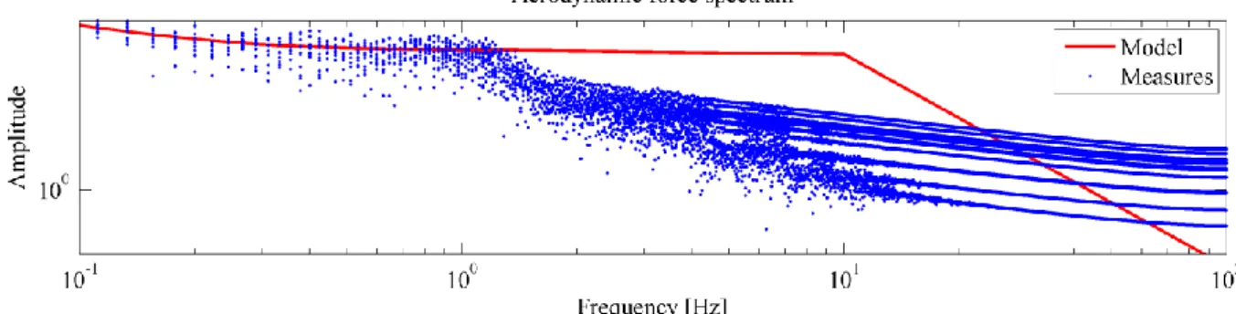
As seen previously, measured aerodynamic-forces are filtered at very low frequency. While defining a probability distribution for the aerodynamic force would be a classical approach, it does not contain any spectral information so that a second approach was preferred here. This proposed method first extends the measured force spectrum to higher frequencies as shown in figure 3. Once this target spectrum defined, a random signal is generated and the perturbation is applied as a time dependant vertical load on the upper mass of the pantograph model.
Figure 3 Aerodynamic force spatial spectrum measured (blue) and spectrum shape defined (red)
4. CONTACT FORCE ANALYSIS
Directly comparing temporal contact forces does not give a clear understanding of the impact of irregularities in particular due to the presence of phase differences with the measurements. To address this issue different comparison tools have been considered. Of the four detailed here, two are used to compare signals together, and two are used to compare signals to measurements.
4.1. Criteria selection
Statistic values
The main goal of pantograph-catenary simulation is to evaluate the current collection quality. The usual approach for this is to divide the variance by mean contact force, which has to be as low as possible, under 0.3 to meet standards. This is a statistical criterion, which defines probability of less than 1% to lose contact supposing the load follows a normal distribution. For each type of irregularity, simulation results will summarized in tables through three standard deviations and one difference of means:
S1= (Fm), with Fm the mean contact force,
S2 = (Fc)), with Fc the time signal of contact force,
S3 = ((Fc)/Fm),
Min3=Min((Fc)/Fm),
Max3=Max((Fc)/Fm),
M3= E((Fc)/Fm),
Mnom= (Fc, nominal)/Fm, nominal.
Spectrum of differences
In order to compare simulations together more precisely than a simple scalar criterion, the computation of the difference between two contact forces gives information about which frequency is more affected by modifications applied. All simulations are compared with the nominal model. For each type of irregularity, results are averaged over a hundred simulations.
FBA:
Frequency Band Analysis (FBA) is a comparison tool used to get a sharper discrimination of unsynchronized signals than a simple comparison of Power Spectral Density (PSD) without observing shift of frequency but only mean amplitude in frequency bands. More explanations are given in [3] and [4]. This tool gives a graphic
analysis of variance against frequency. Defining a range of variation over a set of simulations gives information about the amplitude of variation of energy in a band of frequency, which can easily be compared with measurements. In our case, frequency bands will be centered on the median span frequency harmonics, which appeared to be the main contributors in the PSD. Surfaces with transparency represent the range between maximum and minimum observed values for corresponding set of simulations (in blue) and measurements (in red). Nominal behavior is shown in green.
Frequency coherence function [4] [5]:
The aim of the coherence function, given in (4.3), is to assess and quantify if a linear relationship exists between two sets of frequency spectrums.
In practice, each signal is decomposed in I buffers of equally spaced samples centered on a post. Inter and auto spectrums are then computed as the mean over the I buffers
𝑆
𝑥𝑦𝑓
𝑘=
1𝐼∙ 𝑋 𝑓𝑘;𝑖 ∙𝑌 𝑓𝑘;𝑖 ∗ 𝐼 𝑖=1 (4.1) with 𝑋 𝑓𝑘; 𝑖 = 𝑥 𝑛; 𝑖 ∙ 𝑒−𝐽 ∙ 2𝜋 ∙𝑓𝑘 𝑁∙𝐹𝐸 𝑁−1 𝑛=0 (4.2) and the coherence is given by𝛾𝑥,𝑦2 (𝑓𝑘) = 𝑆𝑦𝑥(𝑓𝑘) 2 𝑆𝑥𝑥(𝑓𝑘) ∙ 𝑆𝑦𝑦(𝑓𝑘) (4.3) where
X is the discrete Fourier transform of the time signal x,
FE is the sample frequency,
fk is the frequency of evaluation of the coherence function,
x,y2(fk) is the coherence function (without units) between x and y at frequency fk,
Sxy(fk) is the Cross Power Spectrum between the signals x and y at frequency fk,
Sxx(fk) Power Spectrum of the signal x at frequency fk,
Since the model and test are random, one has l simulation and m measurements. The final coherence at a frequency is the average l x m coherences. The curve will be shown in black. The process is repeated for each measurement with respect to all others and the average curve is shown in red. It is assumed that simulation coherence with measurements cannot be higher than measurements with each other. To be able to compare with nominal results (i.e. with no irregularity), its coherence with measurements is shown as a green line.
As the numerator is the magnitude squared of a cross power spectrum and the denominator a multiplication of two power spectrum (real valued), the coherence function is real and has a range of between 0 (no linear relationship between the two signals) and 1 (perfect linear relationship between the two signals). The result is usually given in percentage.
In order to be able to compare easily the impact of irregularities, a scalar is introduced as the surface under the curve defined by x,y
2
(fk) for frequencies between 0 and 20Hz. It represents the percentage of coherence between the group of simulations and the group of measurements for this range of frequencies.
4.2. Results
Simulations are done with OSCAR for a nominal model containing 3600 elements and 3200 nodes, for one section with 10 spans of the 14 spans composing the canton. Train speed is fixed at 320km/h with a simulation over 700m. Time consumption is about 2 minutes, which let the possibility to make 300 simulations for all irregularity cases in around 10 hours.
Simulation comparisons
The first result is given in Table 1. M3 - Mnom gives the mean impact of irregularities on current collection
quality (M3 must be as near to zero as possible). Range of variation defined by Min3 and Max3 gives additional
information of the tendency. Geometric irregularity has a strong impact on current collection quality, which can be good or bad. Wear irregularity has no negative impact on current collection and seems to improve it for high level of wear. Aerodynamic irregularity has a low impact on current collection and can be either good or bad.
The S1 and S2 criteria were introduced to analyze sensitivity of mean force and force variance separately. One
can see that aerodynamic irregularity induce principally a variation of the mean represented by S1 and does not
impact local dynamic interaction.
These criteria have to be used all together to compare the different irregularities because they do not follow the same probability distribution.
Table 1 Results of statistical values of sets of contact forces simulated
S1 S2 S3 Min3 Max3 M3 Mnom
Geometric irregularity 0.18 1.31 0.010 0.2111 0.2638 0.2392
0.2408
Wear irregularity 0.09 1.39 0.010 0.1673 0.2414 0.2398
Aerodynamic irregularity 1.66 0.074 0.003 0.2351 0.2507 0.2411
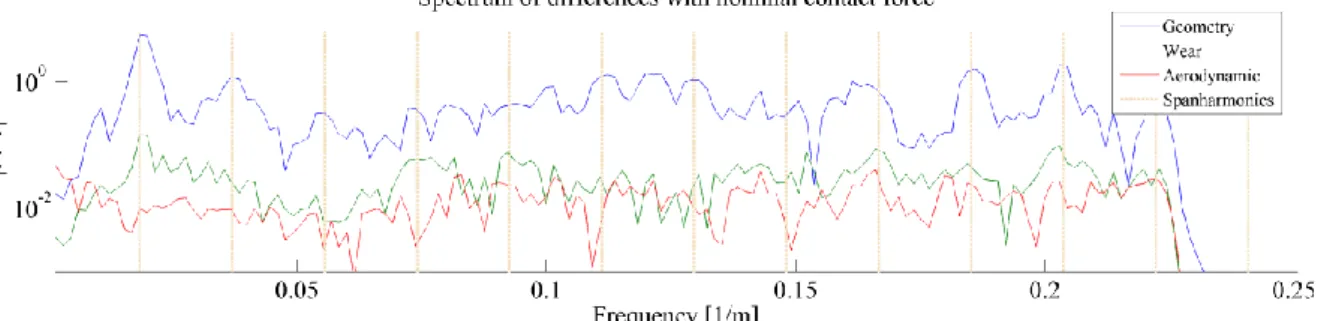
The second result, given in Figure 4, shows the spectrums of contact force differences for each irregularity. Span frequency and harmonics are given with vertical brown dot lines. It appears that the impact of geometric irregularity is focused on span frequencies, which is consistent with the fact that the energy of contact force is higher at these frequencies. It is although not the case of wear and aerodynamic irregularities. This observation confirms the previous conclusion about the lower impact of aerodynamic irregularity than the others.
Figure 4 Mean of spectrums of contact force differences for geometry (blue), wear (green) and aerodynamic (red) irregularities, with span harmonic frequencies (brown)
Measurements-simulations comparison
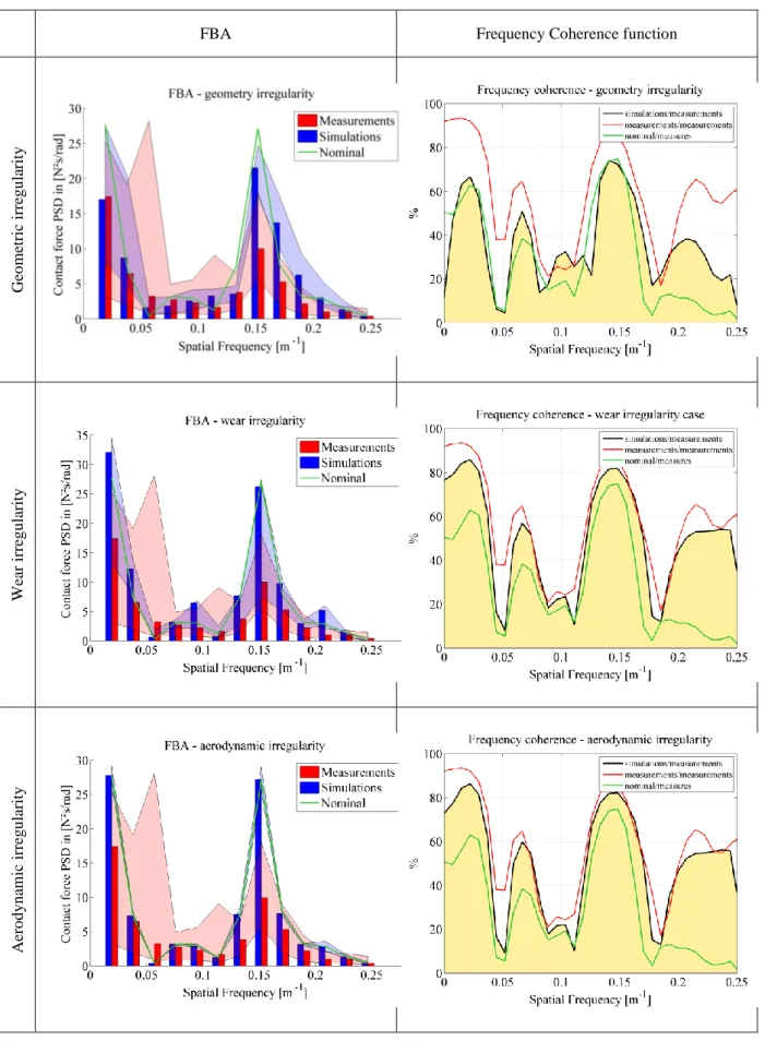
In order to compare variations introduced with variations observed in measurements, the FBA and coherence criteria give visual support.
On FBA graphs (Table 3), one can see the energy variation of the contact force at a specific frequency, namely, the range of variance at this frequency. Geometric and wear irregularities here represent far better, in blue, the amplitude of variations observed in measurements than the aerodynamic one. For frequencies higher than 0.1m-1, wear irregularity seems to be the most representative. The low level of FBA variability in the aerodynamic sensitivity analysis is coherent with the low level of spectrum differences in Figure 4.
On frequency coherence charts, frequency dependent spectrum linearity is assessed between the set of measurements and the set of simulations. Wear and aerodynamic irregularities clearly improve global coherence, which means that phase and frequency variations induced are representative of measured variations unlike what happens with geometry irregularity.
Table 2 Percentage of coherence for each type of irregularity
Mean Coherence between [0-20]Hz Simulations/ Measurements Nominal/ Measurements Measurements/ Measurements Simulations/ Simulations Geometric irregularity 37.81% 32.13% 58.11% 66.02% Wear irregularity 50.13% 95.39% Aerodynamic irregularity 50.82% 96.76%
Values of the scalar coherence criterion, given in Table 2, are closer to the measurement/measurement coherence for aerodynamic and wear irregularities. Other results need a deeper study on this coherence criterion before getting any conclusion, which is beyond the scope of this paper. Anyway, information given by the coherence analysis does not lead to the same conclusion as those by the FBA. It thus deserves to be dealt with in depth.
Table 3 FBA and Coherence graph for each type of irregularity
FBA Frequency Coherence function
Geo m etr ic ir reg u la rity W ea r ir reg u lar ity Aer o d y n am ic ir reg u lar ity
5. CONCLUSION
This first attempt at studying variability in pantograph/catenary simulations shows conclusions about the impact of three different types of irregularities:
Geometry irregularity induces variations of amplitude that are representative of measurements but does not improve coherence with measurements. The defined mean M3 compared to Mnom shows that this kind of
irregularity might increase current collection quality.
Wear irregularity is the most representative of the three, with a significant improvement of coherence and a good range of variation on FBA. Simulations show that this irregularity must be analyzed in detail as it deteriorates current collection quality.
Aerodynamic irregularity as defined here does not affect amplitude variations observed but brings non-linear variations, which are near those observed in measurement. As the energy variation of load is low, this kind of irregularity does not affect current collection quality.
This paper is a relatively simple example showing the importance of introducing variability in current pantograph catenary models. In the near future, more thorough analyses will be led to quantify uncertainties. More sources of variability will be taken into account; measurements will be interpreted with more careful statistical approaches; sensitivity analyzes will allow to relate variability sources and their impact on various criteria.
References
[1] BALMES E., BIANCHI J.-P., MASSAT J.-P., OSCAR 1.0 user's guide, SDTools/SNCF internal report, 2011
[2] BRUNI S., BUCCA G., COLLINA A., Pantograph-catenary dynamic interaction in the medium-high
frequency range, IAVSD n.18, 2004, vol. 41, pp. 697-706.
[3] MASSAT J.-P., LAURENT C., Simulation Tools for Virtual Homologation of Pantographs, International Conference on Railway Technology, 2012.
[4] UNIFE, PantoTRAIN WP3 Deliverable 3.2, internal report, May 2012 p. 89 - 93 and p. 93 - 100
[5] ANTONI J., Cyclostationarity by examples, Mechanical Systems and Signal Processing, Volume 23, Issue 4, May 2009.