An adaptive neighborhood search algorithm for optimizing stochastic mining complexes

(1)

Université de Montréal

Algorithme de recherche à voisinage adaptatif pour

l'optimisation stochastique des complexes miniers

An adaptive neighborhood search algorithm for optimizing

stochastic mining complexes

par Sean Grogan

Département d’Informatique et Recherche Opérationnelle Faculté de Arts et Sciences

Mémoire présenté

en vue de l’obtention du grade de Maîtrise en Informatique

(2)

(3)

Résumé

Les métaheuristiques sont très utilisées dans le domaine de l'optimisation discrète. Elles permettent d’obtenir une solution de bonne qualité en un temps raisonnable, pour des problèmes qui sont de grande taille, complexes, et difficiles à résoudre. Souvent, les métaheuristiques ont beaucoup de paramètres que l’utilisateur doit ajuster manuellement pour un problème donné. L'objectif d'une métaheuristique adaptative est de permettre l'ajustement automatique de certains paramètres par la méthode, en se basant sur l’instance à résoudre. La métaheuristique adaptative, en utilisant les connaissances préalables dans la compréhension du problème, des notions de l'apprentissage machine et des domaines associés, crée une méthode plus générale et automatique pour résoudre des problèmes.

L’optimisation globale des complexes miniers vise à établir les mouvements des matériaux dans les mines et les flux de traitement afin de maximiser la valeur économique du système. Souvent, en raison du grand nombre de variables entières dans le modèle, de la présence de contraintes complexes et de contraintes non-linéaires, il devient prohibitif de résoudre ces modèles en utilisant les optimiseurs disponibles dans l’industrie. Par conséquent, les métaheuristiques sont souvent utilisées pour l’optimisation de complexes miniers. Ce mémoire améliore un procédé de recuit simulé développé par Goodfellow & Dimitrakopoulos (2016) pour l’optimisation stochastique des complexes miniers stochastiques. La méthode développée par les auteurs nécessite beaucoup de paramètres pour fonctionner. Un de ceux-ci est de savoir comment la méthode de recuit simulé cherche dans le voisinage local de solutions. Ce mémoire implémente une méthode adaptative de recherche dans le voisinage pour améliorer la qualité d'une solution. Les résultats numériques montrent une augmentation jusqu'à 10% de la valeur de la fonction économique.

Mots-clés : recuit simulé, métaheuristiques adaptatifs, optimisation des mines, incertitude

(4)

Abstract

Metaheuristics are a useful tool within the field of discrete optimization that allow for large, complex, and difficult optimization problems to achieve a solution with a good quality in a reasonable amount of time. Often metaheuristics have many parameters that require a user to manually define and tune for a given problem. An adaptive metaheuristic aims to remove some parameters from being tuned or defined by the end user by allowing the method to specify and/or adapt a parameter or set of parameters based on the problem. The adaptive metaheuristic, using advancements in understanding of the problem being solved, machine learning, and related fields, aims to provide this more generalized and automatic toolkit for solving problems.

Global optimization of mining complexes aims to schedule material movement in mines and processing streams to maximize the economic value of the system. Often due to the large number of integer variables within the model, complicated constraints, and non-linear constraints, it becomes prohibitive to solve these models using commercially available optimizers. Therefore, metaheuristics are often employed in solving mining complexes. This thesis builds upon a simulated annealing method developed by Goodfellow & Dimitrakopoulos (2016) to optimize the stochastic global mining complex. The method outlined by the authors requires many parameters to be defined to operate. One of these is how the simulated annealing algorithm searches the local neighborhood of solutions. This thesis illustrates and implements an adaptive way of searching the neighborhood for increasing the quality of a solution. Numerical results show up to a 10% increase in objective function value.

Keywords: Simulated Annealing, Adaptive Metaheuristics, Mine Optimization, Metal

(5)

List of Tables

Table 1: Economic Parameters of the Model ... 35

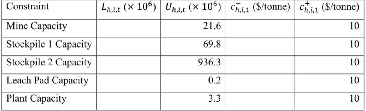
Table 2: Lower and upper bound on constraints (18) and (19) and associated penalties ... 36

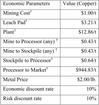
Table 3: Economic Parameters of the Model (Copper) ... 37

Table 4: Lower and upper bound on constraints (18) and (19) and penalties (Copper) ... 38

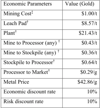
Table 5: Economic Parameters of the Model (Gold) ... 38

Table 6: Lower and upper bound on constraints (18) and (19) and penalties (Gold) ... 39

Table 7: Computer Used ... 39

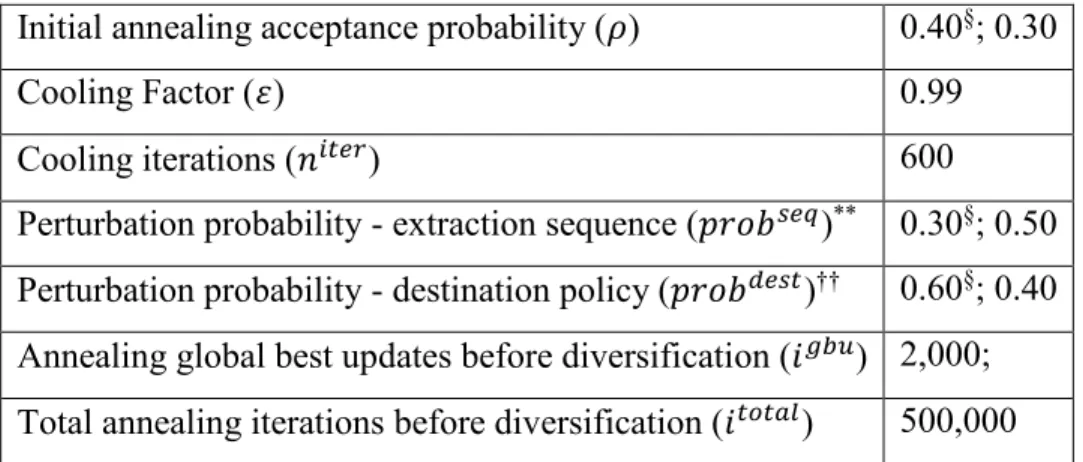
Table 8: Simulated Annealing Parameters ... 40

Table 9: Adaptive Neighborhood Search Parameters ... 40

Table 10: Copper-Gold deposit results ... 42

Table 11: Copper deposit results... 42

Table 12: Gold deposit results ... 42

Table 13: Copper-Gold deposit results with no starter schedule ... 43

Table 14: Copper-Gold Deposit with Differential Evolution ... 45

(8)

List of Figures

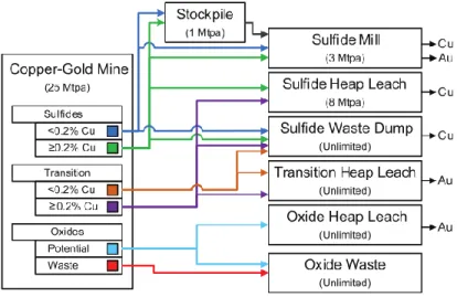
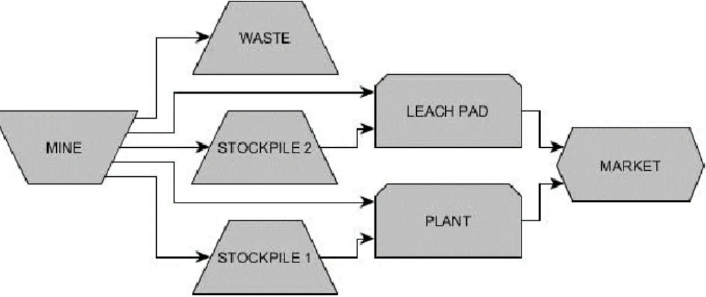
Figure 1: An example of a mining complex ... 4 Figure 2: A 2D schematic of blocks that must be removed to access block 𝑏 ... 5 Figure 3: Definition of material types at the copper-gold mine, along with the various destinations (Goodfellow & Dimitrakopoulos, 2016) ... 35 Figure 4: Illustration of the complexes associated with the single element deposits ... 36

(9)

List of Algorithms

Algorithm 1: Simulated Annealing ... 13

Algorithm 2: Basic adaptive framework as posed by Pisinger & Ropke (2007) ... 16

Algorithm 3: Iterating Simulated Annealing many times ... 27

Algorithm 4: Simulated annealing as developed by Goodfellow & Dimitrakopoulos (2016) . 28 Algorithm 5: Simulated annealing with an adaptive neighborhood search method for optimizing stochastic mining complexes ... 33

Algorithm 6: Initialization and Generation ... i

Algorithm 7: Simulated Annealing with Adaptive Neighborhood Search to solve the two-stage stochastic open pit mining problem ... i

Algorithm 8: A singular execution of a simulated annealing metaheuristic ... ii

Algorithm 9: Setting the initial scores and probabilities for the search neighborhood ... ii

Algorithm 10: Computing the probabilities using scores gained from the simulated annealing iterations ... ii

Algorithm 11: Executing a single iteration of the simulated annealing algorithm ... iii

Algorithm 12: An algorithm that chooses a neighborhood which to perturb the solution and yield a neighborhood solution. ... iii

Algorithm 13: Global optimization of mining complexes ... iv

Algorithm 14: Simulated Annealing for open pit mining complexes ... v

Algorithm 15: Solution perturbation ... vi

Algorithm 16: downstream optimization using PSO or DE ... vi

Algorithm 17: PSO update for particle q ... vii

Algorithm 18: DE for agent q ... vii

(10)

List of Acronyms

ANS: Adaptive Neighborhood Solution APF: Acceptance Probability Function Ag: Silver

Au: Gold CF: Cash Flow Cu: Copper

DE: Differential Evolution GI: Global Iteration IP: Integer Program LOM: Life of Mine LP: Linear Program NPV: Net Present Value ObjFn: Objective Function

PSO: Particle Swarm Optimization

GD: Goodfellow & Dimitrakopoulos (2016) RS: Random Start

SA: Simulated Annealing SIP: Stochastic Integer Program

(11)

All spiritual growth comes from reading and reflection. By reading we learn what we did not know; by reflection we retain what we have learned. The conscientious reader will be more concerned to carry out what he has read than merely to acquire knowledge of it. In reading we aim at knowing, but we must put into practice what we have learned in our course of study. Isidore de Seville

(12)

Remerciements

I would first like to thank Prof. Jacques Ferland for the opportunity to study here at the Université de Montréal and for his guidance in the creation of this thesis. Next, I would like to thank Amina Lamghari for her help also in writing and creating the new method established in this thesis. Furthermore, thanks to Professor Roussos Dimitrakopoulos for opening up this field to me and presenting me with the chance in my Undergrad to be exposed to more advanced ideas in the mining industry.

In addition, I would like to thank a few of my colleagues and mentors from over the years: Ryan Goodfellow, Luis Montiel Petro, Maria Fernanda Del Castillo, Chotipong Somrit, Alessandro Navarra, Hani Mitri, John Mossop, Ryan Lechner, Linda Muratore, Michael O’Boyle, and Mercedes Brand. You guys served as great role models and teachers. You all were generous in sharing your expertise over the years.

Most importantly, I wish to thank my family members: My Mom, Dad, sister Maura, grandmothers Alice and Synnie, and grandpa William. Without your support over the last twenty-six years I would have never been able to get to where I am today. Thank you!

Finally, I would finally like to thank my friends – my extended family in COSMO and Challenge; you have kept me grounded, sane, on track, and fed through the past two years. Many of you have been excellent confidants and mentors, done little things to improve my quality of life, and even directly aided me with this thesis. Thanks to all of you!

(13)

1 Introduction

Mining and related industries is one of the largest and riskiest sectors of the Canadian economy. In 2015, mining and related industries was the third largest industry in Canada after real estate and manufacturing, representing about 8% of the economy, and accounting for 28% of all goods producing industries. In the province of Québec, metallic mineral production represents 26% of the nation’s mineral production (by dollars) and is second only to Ontario (Natural Resources Canada, 2016; Énergie et Ressources Naturelles Québec, 2016; Statistics Canada, 2016). Proper planning procedures and interpretations can mitigate the risk associated with developing and operating mines and mining complexes around the world. In the latter half of the 20th_{century, new ways of modelling mining complexes and interpreting what is in the}

ground have been developed. Furthermore, mathematical models, such as integer programs (IP), have been developed and implemented to schedule the production in mining complexes. As mathematical formulations grew to be more detailed representations of mining complexes, metaheuristics have been developed to efficiently solve them. One such metaheuristic is simulated annealing (SA). SA is used by Goodfellow & Dimitrakopoulos (2016) to optimize their updated model formulation for mining complexes. Their model specifically introduces the ability to account for the “inherent non-linearity related to the blending and stockpiling of materials” (Goodfellow & Dimitrakopoulos, 2016). Their work is based on and updates work of several authors such as Ramazan & Dimitrakopoulos (2013), Jewbali (2006), and Benndorf & Dimitrakopoulos (2004). The SA based optimization method outlined by the authors takes static search parameters for neighbor solution selection. While the authors are able to find a good solution in a reasonable amount of time, this thesis takes progress made in adaptive metaheuristics and related fields, such as from Pisinger & Ropke (2007) and Lamghari & Dimitrakopoulos (2015), to improve the optimization method used by Goodfellow & Dimitrakopoulos (2016). This update to the solver should produce better solutions.

(14)

in extracting naturally occurring and nonrenewable resources. This can be, but is not limited to: gold, copper, potash, uranium, or the oil sands. In addition, mining includes operations that occur after extraction. Examples of these downstream operations include refineries, smelters, and transportation, which transform the extracted material to something more useful (Government of Canada, 2016). We use “more useful” here colloquially. Material is deemed to have been “transformed into something more useful” if the material is transformed, typically called processed, into another material which is closer to something that can be used by a consumer or another industry. Examples are oil into gasoline for a car or insitu copper ore into a copper block to be used by a pipe company. Mining companies operate in areas where they have identified a deposit of material. For this thesis, a deposit is where the companies have deemed there exists material which is economically feasible to be extracted and sold. That is, they can operate a mining complex at a profit. A mining complex is the system by which material is moved from the earth, transformed if possible, and then sold (Blechynden, Gardener, & Mossop, 2012; Government of Canada, 2016; Newman, et al., 2010).

Before a mining complex is established, the deposit must be located. Locating and gaining information about a deposit is known as exploration. There are many different techniques to locate a deposit. Once a company has found a potential area for a mining complex, they must begin a technique known as core hole drilling. Core hole drilling is when machines drill long vertical holes into the earth and retrieve long solid pieces of rock. These long pieces of rock are known as core holes. In the region the company desires to extract material, hundreds to thousands of these core holes will be extracted in a regular grid. These core holes can be viewed as conditioning data for geologists to interpret what is within the earth (Blechynden, Gardener, & Mossop, 2012; Buro, 2013; Newman, et al., 2010). Geologist interpretations are commonly known as orebody models which are ultimately used in planning mine complexes.

In the mine planning, scheduling, and optimizing process, the orebody models are typically discretized into regular sized blocks. This modified model is often referred to as a

block model. For each block in a block model, a geologist will assign an attribute which

represents the amount of a specific material as a proportion by weight. This attribute is known as the grade of the block. Often, the grade is a percentage. For example, a block that weighs

(15)

such as gold or platinum, have small amounts of the metal present in a given block. These metals are typically recorded in grams per tonne. Detailed block models and multi-element deposits will have many attributes in each block. For example, due to molecular similarities, gold deposits will often have economical amounts of silver or copper in addition to gold. Deleterious, or waste, elements are also present. Often copper or gold deposits will have amounts of sulfides, a common deleterious element, present in each block (Buro, 2013; Newman, et al., 2010).

Once a geologist provides a block model interpretation, mine planners must decide how to extract the valuable material at a profit for the company. The first decision a mine planner must make is what kind of mine to establish. There are two basic types of mines: open pit and

underground mines. Open pit mines are developed in places where valuable material is close to

the surface of the earth. They proceed with extracting material at the surface of the earth and continue to work their way deeper until all the valuable material has been extracted. With open pit mining, large amounts of waste material must be removed to gain access to valuable material. In underground mining, on the other hand, is where valuable materials typically extracted through tunnels or shafts. This allows access to valuable material deeper in the earth and reduces the amount of waste material required to be removed if open pit mining techniques were used (Blechynden, Gardener, & Mossop, 2012; Newman, et al., 2010). This thesis will focus on open pit mining. Open pit mining accounts for the largest number of mines in the world and the industry partners we are working with have offered their deposit data, all of which is set up as an open pit mining operation.

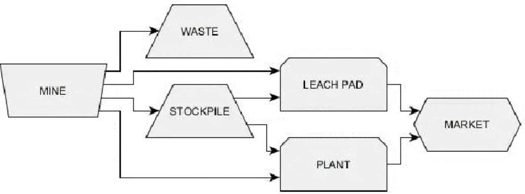
The next decision the mine planner must make is how to move the material through the mining complex. In open pit mining, a mining complex typically has four main locations. The first main location is the physical mine itself. The mine is where the material (blocks) is being extracted from the earth. Once extracted, the blocks are transported to one of three destination locations: a waste dump, a processor, or a stockpile. The decision on where to send each block is based largely on the grade of the block. Blocks sent to the waste dump typically lack sufficient quantities of valuable material to be processed and sold at any kind of advantage for the

(16)

material to something more useful. The output of a processor typically has the ability to be sold at a market or to a contracted firm. In a copper or gold mine, there are two types of processors. The first processor type is a plant. A plant will attempt to grind ore material into a fine powder and use a separation technique, such as flotation, to separate waste material from the valuable material. The flotation happens in a modified water solution where the properties of the water are chemically adjusted in such a way where valuable material will stick to air bubbles and float to the top of a flotation cell while waste will settle to the bottom. The second processor type is a leach pad where acid is used to “leach” away valuable material from waste material. The third possible destination for extracted material is a stockpile. Stockpiles are areas that companies set aside to store material until there is an opportunity to process it. Stockpiling material is due to limitations in the amount of material that can be processed or a desire to blend material at a processor to increase the advantage to a company. Blending material is processing two units of different material at the same time to get the average of the material’s properties. An outline of the basic mining complex and the main destinations can be seen in Figure 1 below (Blechynden, Gardener, & Mossop, 2012).

Figure 1: An example of a mining complex

As mentioned above, a processor attempts to separate the waste material from the valuable material. This separation is not perfect. For each processor, there is an associated value called the recovery, which represents a percentage that is the amount of valuable material that is saved, or recovered, from each block. For example, if a plant has a 90% recovery, a block with 150 tonnes of copper will yield 135 tonnes of the copper out of the plant. The other 15 tonnes will be discarded. Compare this with a leach pad that has a 50% recovery; that same

(17)

typically a function of the amount of material and/or the grade of the material sent to the processor. Therefore, the recovery of a processor is often non-linear and can vary on a variety of factors (Blechynden, Gardener, & Mossop, 2012).

There are two main constraints in an open pit mining complex. The first are the capacity

constraints. Equipment, safety, and other limitations exist which restrict the amount of material

that can be moved or processed at each part of the complex in a given period. A period is a unit of time, typically a year, that a mine complex is operated. Capacity constraints take a few forms.

Mining capacity is the amount of material that can be extracted from the mine in a period. Processing capacity is the amount of material that can be sent to a specific processor in a period. Stockpiling capacity is the amount of material that can be stored in a stockpile. While mining

and processing capacities are calculated on a per period basis, the stockpile capacity is the upper limit on the amount of material that can be stored there at any given time. The sum of all the material is carried over period to period until it is rehandled, or moved again – in this case from the stockpile to the processor (Newman, et al., 2010).

In addition to capacity constraints, precedence constraints exist in open pit mining complexes, sometimes called slope constraints in the literature. In open pit mining when scheduling with a block model, for a given block, the block directly above and blocks adjacent to the directly above block must be extracted before the given block can be. An example of this can be seen in Figure 2 below.

(18)

Block 𝑏 (the block highlighted in light grey) can be extracted. Note that we will use slopes of

45° in the examples in this thesis. However, slopes may take a variety of angles for geotechnical or other safety reasons. It is these precedence constraints which often make optimizing mining complexes quite long and complicated (Newman, et al., 2010).

1.2 Mining Complex Economic Evaluation

After core holes have been extracted and before a company decides to establish a mining complex, the company will conduct a feasibility study to determine the economic value of the deposit and complex. One part of the feasibility study is to schedule material movement in the mining complex, which is what the formulation and the solution method in this thesis can be applied to. Planners will attempt to maximize this economic value over the course of the life of

mine (LOM). The LOM is the number of periods from the beginning of development of the

project until there remains no more material in the deposit or stockpiles that can be processed at an advantage for the company. Note that the LOM and economic evaluation of a mine will typically not include the exploration and core hole drilling costs and procedures. However, the economic evaluation will often include other capital expenditures such as the construction of plants and the purchase of equipment. The exception to including capital expenditures is if a new mine is being developed in the vicinity of an already established mining complex where equipment can simply be moved or be used in multiple complexes (Albach, 1967; Blechynden, Gardener, & Mossop, 2012; Gentry, 1988).

Most mining projects calculate the economic advantage with a criterion known as net

present value (NPV). Broadly speaking, the NPV is the value of a project. An NPV with a

positive value indicates that the projected earnings generated by a project or an investment exceed the anticipated costs when taking the value of money over time into consideration. The NPV of a mining project is calculated as follows:

1) Calculate the cash flow (CF) of each period for the entire LOM. The CF of a period is typically the value of the material sold, minus the costs incurred to process and transport the material.

(19)

2) Determine the discount rate of the project. This discount rate is a percentage that is associated with a project which encompasses the risk of a project and the rate of return from other possible investments. It is typically determined from other similar projects and the state of the economy.

3) For each period, determine the present value (PV) of the CF for each period. The PV is calculated by dividing the CF of the period by one plus the discount rate raised to the number of periods from the first period. I.e. PVt = CFt⁄(1 + discount rate)t. This can

be viewed as the CF at time 𝑡 has a value of PV_t today.

4) Sum all the PV’s for each period to get the NPV of the project: i.e. NPV = ∑_𝑡∈𝕋PV_𝑡 Other evaluation methods can be used, but NPV is the most common and widely understood in the industry (Gitman & Joehnk, 1999; Investopedia, 2016; Whittle, 2014).

The factors that go into determining the value of a CF in a period are the costs associated with extracting, moving, and processing material from a mine to the three destinations and the value of the material sold on the market. Recall we are operating an open pit mine and there are precedence constrains associated with extracting a block. Looking back to Figure 2 on page 5, imagine if block 𝑏 was the only block that had valuable material in it and all the overlying blocks in the set 𝕆𝑏 were waste material. We must extract and incur the cost associated with removing

the 8 blocks in the overlying block 𝕆_𝑏 set in addition to the cost of extracting, processing, and subsequently selling block 𝑏. We only see revenue in the period after block 𝑏 is processed and then sold.

Mining projects are quite a high risk investment. These projects typically have a few unique attributes compared to other investment opportunities. They are:

 Capital intensive projects – they have a high initial starting cost.

 Non-renewable resource – Once the material is extracted, it is gone from the Earth. Any infrastructure built is typically abandoned or sold at a significant loss if the mine is in a remote location.

(20)

 Long pre-production periods – it may take several periods for unwanted material to be extracted to get to valuable material. In addition, infrastructure, such as roads and plants, may need to be built to handle the material.

 The indestructibility of the material – gold mined in Quebec will be essentially the same as gold from Nevada or Ghana. Therefore, one can seek either cheaper deposits elsewhere or look in low risk locations.

The combination of these factors makes mining a high risk environment for investors. Therefore, proper planning and evaluation is critical for investors and companies to make informed decisions about mining projects (Gentry, 1988; The Northern Miner, 1990; Whittle, 2014).

1.3 Optimization of Open Pit Mining Complexes

Traditionally, mining complexes were scheduled both locally and iteratively. We say locally because each location and element in the mining complex was independently scheduled. This is akin to a greedy heuristic and can lead to a sub-optimal global solution. Recall we are attempting to maximize NPV. An example of the local scheduling technique can be to maximize recovery of a processor. Maximizing the recovery of a processor ensures the most amount of valuable material is sent to the market (least amount of valuable material is wasted). However, this greedy local decision to maximize recovery may lead to a sub-optimal decision. Typically, a higher recovery reduces the rate at which material can be processed in the plant (i.e. the processor operator must lower processing capacity), but increasing the processing capacity of the processor and lowering recovery, may increase the overall NPV. A mining complex is considered to be scheduled iteratively because a small change in one part of the mining complex can affect the value of the complex as a whole. Using an example as an illustration, let there be a plant engineer who decided to plan for the processing capacity to be 𝑃𝐶1. If we change the

processing capacity from 𝑃𝐶₁ to a lower value 𝑃𝐶₂, the engineers who manage extraction scheduling must adjust the amount of material they send to the processor; by sending some material as waste, by opening a stockpile to store excess material, by reducing the mining capacity, or by changing which blocks are mined in each period. Once the schedule is updated,

(21)

planners may then decide to make another small adjustment to the mining complex parameters and then the process repeats (Gentry, 1988; The Northern Miner, 1990; Whittle, 2014).

Because of this local and iterative process for determining a schedule to extract material over the life of mine, we desire a global way to optimize these complexes. That is, we desire a way to simultaneously optimize production scheduling. This led to the development of linear and integer programs to represent the production schedule. These mathematical formulations have the ability to choose the best extraction scheduling decisions. These methods were first explored in the 1960’s (Albach, 1967; Gershon, 1983; Gholamnejad & Osanloo, 2007; Bienstock & Zuckerberg, 2010; Busnach, Mehrez, & Sinuany-Stern, 1985). Due to the wide range of mines in the world and how basic concepts are applicable across many deposits and complexes, mine complex optimization is a well-studied field (Newman, et al., 2010). Some of the most modern methods do incorporate what is known as metal uncertainty.

1.4 Metal Uncertainty and the Simulation of Orebody Models

Because mining complexes are developed based on the information obtained from core hole drilling, the interpretation of what is in the deposit can have a significant impact on the valuation of a mining complex. Traditionally, mining complexes were optimized using a singular orebody model. This model was developed using an interpolation method, such as kriging (Krige, 1951), between the known data points, the core holes. These traditional methods smooth the transition of grades between the core holes. This incorrect estimation will lead to an inaccurate and high-risk evaluation of a deposit (Ravenscroft, 1992; Godoy M. , 2003; Dimitrakopoulos, 2015; Consuegra & Dimitrakopoulos, 2009; Dimitrakopoulos, Farrelly, & Godoy, 2002; Osterholt, 2005).

Geostatistical or stochastic conditional simulation is an estimation tool which generate

models of a deposit based on the same core hole data used in traditional methods. When one generates multiple simulated orebody models, they take on two properties (Dimitrakopoulos, 2015):

(22)

1. Simulations reproduce the available information of the core holes. That is, the simulations will reproduce similar information that is already represented by the core holes.

2. Each simulation is an equiprobable representations of the deposit.

Examples of simulation methods that are used are direct block simulation, Gaussian simulation methods, and high order simulation methods (Benndorf & Dimitrakopoulos, 2004; Godoy & Dimitrakopoulos, 2004). Authors who optimize using simulated orebody models typically find a higher NPV and a lower risk schedule when compared to using a single orebody model. For example, Goodfellow & Dimitrakopoulos (2016) use a stochastic integer program (SIP) to represent the mining complex. This model was able to achieve an NPV 6.6% higher than the deterministic model. In addition, less risk is associated with the amount of material sent to various destinations. Another example is by Dimitrakopoulos, Farrelly, and Godoy (2002) who perform a risk analysis on a mine. Their analysis shows that when using simulated orebodies, the deterministically scheduled mine has only 15% chance of reaching the original NPV. Additionally, the authors conclude that the expected NPV of the schedule is 25% below what is originally projected using the deterministic model. A third case study is where Godoy (2003) completes a risk analysis for a mine in Australia. Results of using simulated orebodies yields a 28% increase in NPV compared to the deterministic solution and a 3% chance of the stochastic schedule failing to meet yearly production targets, as opposed to the 13% for the deterministic schedule. The author notes that the increase in NPV is due to the optimizer’s ability to extract more valuable material earlier in the life of mine.

This thesis will utilize simulated orebody models in the optimization process.

1.5 Objectives of the Research

In this thesis, we refer to a recent and more general mathematical formulation representing a mining complex – the act of moving raw material from the earth to selling refined material on the market – presented by Goodfellow & Dimitrakopoulos (2016). In order to solve this problem, we also refer to their simulated annealing approach using several neighborhoods to determine a schedule of events through the life of the project. In their implementation, the

(23)

neighborhood used at each iteration is selected among a set of different neighborhoods according to a distribution specified a priori. The main contribution in this thesis is to improve this solution approach by using the adaptive principles introduced in Pisinger & Ropke (2007) and in Lamghari & Dimitrakopoulos (2015) to select the neighborhood. The motivation for this contribution is twofold. Indeed, it allows for a different mining complex to be resolved without having a user to determine a priori the distribution for selecting the neighborhood, and also for a mine planner who may not be familiar with metaheuristic principles, to use this method to develop a schedule for their mining complex. The numerical results show an average increase of 1 to 2% of the objective function value for a single element deposits. For a larger copper-gold deposit, we observe an average increase of 10% for the objective function value and a reduction of about 40% of the solution time.

The remainder of this thesis is organized as follows. The simulated annealing approach and the principles of adaptive metaheuristics are summarized in Chapter 2. Chapter 3 includes the general mathematical formulation of the model introduced in Goodfellow & Dimitrakopoulos (2016). It also includes their implementation of the simulated annealing and the details of the adaptive selection of the neighborhood. The numerical results are summarized in Chapter 4. Two single element deposit problems including copper and gold, respectively, and a larger problem including a copper-gold deposit are solved in order to illustrate the advantage of using the adaptive approach. Chapter 5 includes conclusions.

(24)

2 Review of Metaheuristics and Adaptive Metaheuristics

“Metaheuristics are solution methods that orchestrate an interaction between local improvement procedures and higher level strategies to create a process capable of escaping from local optima and performing a robust search of a solution space” (Gendreau & Potvin, 2010). That is, metaheuristics are a set of algorithms which allow for broad search of solutions, even solutions that are non-improving, to discover high quality solutions. Metaheuristics are a useful tool within the field of discrete optimization that allow for large, complex, and difficult optimization problems, such as the one addressed in this thesis, to be solved in a reasonable amount of time. Solving discrete optimization problems in an exact way may take orders of magnitude longer to solve than using a metaheuristic to reach a good or acceptable solution to the problem. Adaptive metaheuristics aim to increase the generalization of a metaheuristic method for a given problem. This may allow for a user who is untrained in the implementation of a metaheuristic to use the method to find a solution to the problem.

This section outlines the metaheuristics used by Goodfellow & Dimitrakopoulos (2016), specifically simulated annealing (SA). In the solution approach of Goodfellow & Dimitrakopoulos (2016), they use a strategy to optimize downstream (processor) variables after SA. This strategy relies on the population based procedures differential evolution (DE) and particle swarm optimization (PSO). Since we are not modifying these strategies in this thesis, we will not describe their implementation further except for a brief comment on their use in the solving method outlined by Goodfellow & Dimitrakopoulos (2016) in section 3.2.

2.1 Simulated Annealing

Simulated annealing (SA) is a local neighborhood search metaheuristic allowing to modify the current solution even with one deteriorating the objective the objective function value in order to move away from a local optimal solution. Kirkpatrick, et al. (1994) and Cerny (1985) were the first to propose solving combinatorial problems with this approach used in thermodynamics to search for an equilibrium. To ease this presentation, suppose that we are solving the following problem of maximizing a function 𝑓(𝑥) over a feasible domain 𝑋 ∈ ℝ𝑛_.

(25)

solution 𝑥. A neighbor solution 𝑥′_{is typically similar to the current solution, with a few simple}

modifications to the current solution 𝑥. The SA algorithm then allows to compare the quality of the selected solution against the quality of the current solution. If the selected solution is better (i.e. 𝑓(𝑥′_{) > 𝑓(𝑥)), then it becomes the current solution. Otherwise (if the selected}

solution 𝑥′_{is worse), 𝑥}′_{can replace the current solution 𝑥 even if Δ𝑓 = 𝑓(𝑥}′_{) − 𝑓(𝑥) ≤ 0}

according to a function which calculates the probability as a function of Δ𝑓 and the number of iterations already completed; i.e. 𝑥′_{replaces 𝑥 with the acceptance probability function 𝑒}Δ𝑓 τ⁄

where 𝜏 (the temperature parameter) decreases with the number of iterations completed. In this variant, we complete several iterations 𝑛𝑖𝑡𝑒𝑟_{with the same temperature 𝜏. Note}

that a special case is to modify the temperature at each iteration (i.e. 𝑛𝑖𝑡𝑒𝑟 _{← 1). The}

temperature 𝜏 is modified with the parameter 𝜀 (i.e. at 𝜏 ← 𝜏 ∙ 𝜀), where 0 < 𝜀 < 1. Two stopping criteria are used. The first one is specified in terms of the number of iterations the SA is ran (𝑖𝑡𝑒𝑟𝑀𝑎𝑥). The second is one is specified in by counting the number of global best updates

(𝑖_{𝑙𝑖𝑚𝑖𝑡}𝑔𝑏𝑢 ), that is, the number of times a new global best solution is found. A variant of the procedure can be summarized in Algorithm 1.

Algorithm 1: Simulated Annealing

Initialization:

Select an initial solution 𝑥0∈ 𝑋 and an initial temperature 𝜏0

Let 𝑖𝑡𝑒𝑟 ← 0; 𝜏 ← 𝜏0 Let 𝑥 ← 𝑥0; 𝑥∗← 𝑥0

While stopping criteria is not met 𝑖𝑔𝑏𝑢_{← 0}

𝑖𝑡𝑒𝑟 ← 𝑖𝑡𝑒𝑟 + 1

Repeat 𝑛𝑖𝑡𝑒𝑟 times with the same temperature 𝜏 Generate randomly 𝑥′ ∈ 𝑁(𝑥)

Δ𝑓 = 𝑓(𝑥′) − 𝑓(𝑥) If Δ𝑓 > 0

𝑥 ← 𝑥′

Else generate a random number 𝑟 ∈ [0,1] If 𝑟 < 𝑒Δ𝑓 𝜏⁄

𝑥 ← 𝑥′ If 𝑓(𝑥′) > 𝑓(𝑥∗₎

(26)

In order to improve the quality of the solution generated with any local neighborhood search procedure, it should be combined with a diversification strategy to search more extensively the feasible domain of the problem. Many such strategies exist, and they are most of the time specific to the problem.

2.2 Adaptive Neighborhood Search Techniques

One of the difficulties in using metaheuristics in optimization is that often the methods require parameter tuning by the user to increase the quality of the final solution. One promising area of research is utilizing adaptive neighborhood search (ANS) to help guide the search of the solution space. ANS is especially useful when using a metaheuristic which has a local search framework, such as in the case of SA.

In this section, we analyze the step “generate randomly 𝑥′ _{∈ 𝑁(𝑥)” in the SA procedure}

in Algorithm 1. Moreover, consider the case where 𝑁(𝑥) is specified using a set of neighborhoods {𝑛₁, 𝑛₂, … , 𝑛_|ℕ|}. Note that in the SA implementation of Goodfellow & Dimitrakopoulos (2016), the number of neighborhoods |ℕ| is equal to three. Before generating 𝑥′_{, we first select randomly the neighborhood to be used. In Goodfellow & Dimitrakopoulos}

(2016), this section is made by a probability distribution specified a priori and manually tuned by the authors. In the proposed contribution in this thesis, this probability distribution is made adaptive. The probability of selecting neighborhood 𝑛_𝑖 is proportional to its efficiency in the solving process. This approach follows the adaptive large neighborhood search (ALNS) approach outline by Pisinger & Ropke (2007).

The selection process is summarized as follows: At each iteration to generate a neighbor solution 𝑥′, first a neighborhood 𝑛_𝑖 must be selected. 𝑛_𝑖 is selected by an associated probability 𝑝𝑖 for all the 𝑖 ∈ ℕ. The same values of the probabilities 𝑝𝑖, ∀𝑖 ∈ ℕ should be used for the same

number of (𝑆𝑐𝑜𝑟𝑒𝑈𝑝𝑑𝑎𝑡𝑒)𝑆𝑘𝑖𝑝 iterations in the local search method. At each

(𝑆𝑐𝑜𝑟𝑒𝑈𝑝𝑑𝑎𝑡𝑒)𝑆𝑘𝑖𝑝 iteration, the probabilities 𝑝𝑖 should be updated based on a score parameter

(27)

neighborhood. Therefore, larger scores will represent neighborhoods that have a better impact on the quality of the solution.

To update the scores after (𝑆𝑐𝑜𝑟𝑒𝑈𝑝𝑑𝑎𝑡𝑒)_{𝑆𝑘𝑖𝑝} iterations, there is a scalar 𝜅_𝑖 indicating the number of times neighborhood 𝑛_𝑖 is selected. In addition, the value of 𝜋(𝑛_𝑖) represents the efficiency of neighborhood 𝑛_𝑖. The values are updated each time neighborhood 𝑛_𝑖 is selected as follows:

𝜅_𝑖 ← 𝜅_𝑖+ 1 (1)

𝜋(𝑛𝑖) ← 𝜋(𝑛𝑖) + 𝜎 (2)

where 𝜎 represents the value of the efficiency of 𝑛_𝑖. We will calculate the efficiency 𝜎 as a function of the change in the objective function value. After completing (𝑆𝑐𝑜𝑟𝑒𝑈𝑝𝑑𝑎𝑡𝑒)_{𝑆𝑘𝑖𝑝} iterations, the scores 𝑠_𝑖 are updated as follows:

𝑠_𝑖 ←{(1 − 𝛼)𝑠𝑖 + 𝛼(

𝜋(𝑛𝑖)

𝜅_𝑖 ) If 𝜅𝑖> 0

𝑠𝑖 Otherwise

(3)

and the probabilities 𝑝_𝑖 become

𝑝𝑖 ←

𝑠𝑖

∑𝑘∈ℕ𝑠𝑘

∀𝑖 ∈ ℕ (4)

Take note that in (3), if a neighborhood is not called, the score remains the same for the next (𝑆𝑐𝑜𝑟𝑒𝑈𝑝𝑑𝑎𝑡𝑒)_{𝑆𝑘𝑖𝑝} iterations. There is also the introduction of a parameter 𝛼 ∈ [0,1] which controls the emphasis on historical scores versus new scores. That is, if the parameter 𝛼 is set close to 1, more emphasis is placed on newer information versus an 𝛼 closer to 0 which places emphasis on historical information.

In the following chapter, we introduce the model proposed in Goodfellow & Dimitrakopoulos (2016) for an open pit mining complex and their specific implementation of

(28)

An outline of the method described above can be seen here in Algorithm 2. Algorithm 2: Basic adaptive framework as posed by Pisinger & Ropke (2007)

GENERATE 𝑥 # Initial Solution 𝑥 SET 𝑥∗← 𝑥 # Best Solution 𝑥∗

𝑖 ← 0

WHILE Stopping criteria is not met 𝑖 ← 1 + 1

If 𝑖 mod (𝑆𝑐𝑜𝑟𝑒𝑈𝑝𝑑𝑎𝑡𝑒)𝑆𝑘𝑖𝑝 = 0

Update the probabilities 𝑝𝑖 based on scores 𝑠𝑖

Set 𝑠𝑖 ← 0∀𝑖 ∈ ℕ

Choose a neighborhood 𝑛𝑖 probabilities 𝑝𝑖

GENERATE x′ from 𝑥 using the neighborhood 𝑛𝑖

IF 𝑥′ is accepted 𝑥 ← 𝑥′

UPDATE 𝜋(𝑛𝑖) based on success

ELSE

UPDATE 𝜋(𝑛𝑖) based on failure

IF 𝑥 is a better solution than 𝑥∗ 𝑥∗_{← 𝑥}

(29)

3 Implementation of Adaptive Neighborhood Choice in

Simulated Annealing to Optimize the Stochastic Mining

Complex

This section introduces an overview of the model (section 3.1) and the solver (section 3.2) presented by Goodfellow & Dimitrakopoulos (2016). The third part of the section goes over the contribution to include an adaptive neighborhood search in the solving method (section 3.3). This adaptive neighborhood search used in this contribution is based on the work of Lamghari & Dimitrakopoulos (2015).

Recall that a naïve way of scheduling a mining complex is to discretize a deposit into a collection of blocks and to assign a dollar value to each block; this value is calculated by the grade of the block, the recovery value of the processor, costs incurred in processing, and the market value of the metal. This approach to valuing a complex is inaccurate when applying it to a mine in practice. For example, recall the basic mining complex from section 1.1. Each processor has a different recovery and this difference in recovery will result in a different value of the block being mined. Therefore, we must use a model to analyze the value of a mining complex referring to its outputs rather than to each block value.

3.1 Stochastic Integer Model of an Open Pit Mining Complex

Goodfellow & Dimitrakopoulos (2016) utilize a two-stage stochastic optimization model. The formulation, replicated here, is written to be more holistic than models that appear elsewhere in the literature, such as those explored in section 1.3. That is, they aim the model to be able to be applied to a wide variety of deposits with more production constraints. In addition, the model is better at valuing the output of the processor outputs each period rather than the value of each block sent through a processor.

(30)

2. 𝒮: Nodes associated with stockpiles. 3. 𝒫: Nodes associated with processors.

Note that using this notation, a waste dump can also be viewed as a processor that has a recovery of zero, i.e. no value is gained from a “waste dump processor.” Moreover, a cluster 𝒞 is used to group together similar blocks of material in the mine. The authors group material into clusters using a k means++ clustering algorithm. K means++ was used because it generally produces stable clusters relative to regular k means clustering algorithm and a much more diverse cluster sets due to the weighting in the algorithm (Arthur & Vassilvitskii, 2007). The authors operate under the assumption that if two distinct blocks in separate parts of the mine have similar attributes (such as grade of the material or the amount of deleterious elements in a block), the two distinct blocks will have the same destination in 𝒮 or 𝒫. For example, if two blocks have a grade of zero then both blocks will potentially be sent to the same destination – the waste dump. Therefore, we will be making the decision for extracting a block referring to the blocks and its destination is made by referring to its cluster.

In the following notation, material will flow from node 𝑖 ∈ 𝒩 to 𝑗 ∈ 𝒩 (material flows from node 𝑖 to node 𝑗). 𝒪(𝑖) represents the set of nodes that can receive materials from node 𝑖. ℐ(𝑗) is the set of nodes that can send material to node 𝑗.

Indices and sets of the model are:

 𝑚 ∈ 𝕄 is a set of mines within a complex.

 𝑏 ∈ 𝔹_𝑚 is the set of blocks within a mine 𝑚 ∈ 𝕄.

 𝑡 ∈ 𝕋 is a set of time periods, typically years, where |𝕋| represens the life of mine of the complex.

 𝑢 ∈ 𝕆𝑏 is the set of blocks overlaying block 𝑏 ∈ 𝔹𝑚.

 𝑠 ∈ 𝕊 is a set of scenarios that represent a realization (simulation) of all sources of uncertainty. Specifically, for this model it is the uncertainty of the metal grade in a block that is accounted for (metal uncertainty). When using simulated orebody models, each scenario is equiprobable (Dimitrakopoulos, 2015).

(31)

 𝑝 ∈ ℙ represent primary attributes, fundamental variables of interest sent through the model (such as metal content, tonnage). These attributes are typically linked directly with the attributes of the simulation and are always linearly transferred between parts of the mining complex. The value of primary attribute 𝑝 from 𝑖 at time 𝑡 under period 𝑠 is denoted as 𝑣_{𝑝,𝑖,𝑡,𝑠}. These attributes often originate at mines 𝑚 ∈ 𝕄 and may flow through the mining complex to the final products. The value of the attribute recovered after treatment is denoted by 𝑟𝑝,𝑖,𝑡,𝑠.

 ℎ ∈ ℍ represents hereditary attributes. These attributes may be described as linear and non-linear functions of primary attributes, 𝑓ℎ,𝑖(𝑣𝑝,𝑖,𝑡,𝑠), of the primary

attributes. The value of the hereditary attribute ℎ at location 𝑖 at time 𝑡 under scenario 𝑠 is denoted as 𝑣_{ℎ,𝑖,𝑡,𝑠}.

The parameters of the model are defined as follows:

 𝜑_{ℎ,𝑖,𝑡} ∀ℎ ∈ ℍ, 𝑖 ∈ 𝒮 ∪ 𝒫, 𝑡 ∈ 𝕋 represents the discounted revenue or expense associated with hereditary attribute ℎ at a given node 𝑖 in time 𝑡. Typically, with a given economic discount rate 𝑑𝑒, 𝜑ℎ,𝑖,𝑡 =

𝜑ℎ,𝑖,1

(1+𝑑𝑒)𝑡.

 𝑈_{ℎ,𝑖,𝑡} and 𝐿_{ℎ,𝑖,𝑡} ∀ℎ ∈ ℍ, 𝑖 ∈ 𝒮 ∪ 𝒫 ∪ 𝕄, 𝑡 ∈ 𝕋 represent the upper and lower limits, or target, of attribute ℎ at destination 𝑖 in period 𝑡. For example, this could be a processor target.

 𝑐_{ℎ,𝑖,𝑡}+ _{and 𝑐}

ℎ,𝑖,𝑡− ∀ℎ ∈ ℍ, 𝑖 ∈ 𝒮 ∪ 𝒫, 𝑡 ∈ 𝕋 represent the cost (penalty) of deviation

from a target (above and below the upper and lower targets respectively) for hereditary attribute ℎ, at destination 𝑖, in period 𝑡. Here, the authors use a separate discount rate, called the risk discount rate 𝑑_𝑟, to calculate the value of 𝑐_{ℎ,𝑖,𝑡}+ and 𝑐_{ℎ,𝑖,𝑡}− _{. That is, 𝑐}

ℎ,𝑖,𝑡+ = 𝑐ℎ,𝑖,1+

(1+𝑑𝑟)𝑡 and 𝑐ℎ,𝑖,𝑡

− ₌ 𝑐ℎ,𝑖,1−

(1+𝑑𝑟)𝑡.

(32)

determined to be a member of cluster 𝑐, 𝜃_{𝑏,𝑐,𝑠} = 1, otherwise 𝜃_{𝑏,𝑐,𝑠}= 0. It is understood that ∑_𝑐∈𝒞𝜃_{𝑏,𝑐,𝑠} = 1 ∀𝑏 ∈ 𝔹_𝑚, 𝑚 ∈ 𝕄, 𝑠 ∈ 𝕊

In addition to the a priori parameters defined above, there is also a transformation function:

 𝑓_ℎ,𝑖(∗) ∀ℎ ∈ ℍ, 𝑖 ∈ 𝒮 ∪ 𝒫 is a function for the hereditary attribute. This function is defined a priori. What this function does is take a value of a primary attribute 𝑣_{𝑝,𝑖,𝑡,𝑠} and convert it into a hereditary attribute 𝑣_{ℎ,𝑖,𝑡,𝑠}. An example is recovery of metal from a processor.

Goodfellow & Dimitrakopoulos (2016) define three main decision variables in their solution vector. The solution vector is Φ = {𝒙, 𝒚, 𝒛} where 𝒙, 𝒚, 𝒛 represent the decision variables in the stochastic integer program. The variables are defined as follows:

1. Extraction sequence decision variables (𝒙 ∈ Φ): 𝑥𝑏,𝑡 is the extraction sequence

decision variable where 1 represents mining block 𝑏 in period 𝑡, 0 otherwise. 2. Destination policy decision variables (𝒛 ∈ Φ): 𝑧_{𝑐,𝑗,𝑡} is a binary variable where

blocks in cluster 𝑐 are sent to destination 𝑗 in period 𝑡

3. Processing stream decision variables (𝒚 ∈ Φ): 𝑦𝑖,𝑗,𝑡,𝑠 is a continuous variable

between 0 and 1 indicating the proportion of material sent from node 𝑖 to destination node 𝑗 in period 𝑡 under scenario (realization) 𝑠

Goodfellow & Dimitrakopoulos (2016) also define the following as variables whose values depend on both the realization of the metal content and the values of the three variables above.

 𝑣_{𝑝,𝑖,𝑡,𝑠} ∀𝑝 ∈ ℙ, 𝑖 ∈ 𝒮 ∪ 𝒫 ∪ 𝕄, 𝑡 ∈ 𝕋, 𝑠 ∈ 𝕊 represent the value of the primary attribute 𝑝 at a given node 𝑖 in time 𝑡 under scenario 𝑠.

 𝑣ℎ,𝑖,𝑡,𝑠 ∀ℎ ∈ ℍ, 𝑖 ∈ 𝒮 ∪ 𝒫, 𝑡 ∈ 𝕋, 𝑠 ∈ 𝕊 represents the value of the hereditary

attribute ℎ at a given node 𝑖 in time 𝑡 under scenario 𝑠.

 𝜑_{𝑝,𝑐,𝑡,𝑠}∀𝑝 ∈ ℙ, 𝑐 ∈ 𝒞, 𝑡 ∈ 𝕋, 𝑠 ∈ 𝕊 is the quantity of the value attribute 𝑝 in cluster 𝑐 at time 𝑡 under scenario 𝑠.

(33)

 𝑑_{ℎ,𝑖,𝑡,𝑠}+ _{and 𝑑}

ℎ,𝑖,𝑡,𝑠− ∀ℎ ∈ ℍ, 𝑖 ∈ 𝒮 ∪ 𝒫, 𝑡 ∈ 𝕋, 𝑠 ∈ 𝕊 represent the value of

deviation from a target (above and below the upper and lower targets respectively) for hereditary attribute ℎ, at destination 𝑖, in period 𝑡, when scenario 𝑠 occurs.

 𝑟𝑝,𝑖,𝑡,𝑠 ∀𝑝 ∈ ℙ, 𝑖 ∈ 𝒮, 𝑡 ∈ 𝕋, 𝑠 ∈ 𝕊 is a variable to mass balance primary

attributes in the mining sequence. This can be viewed as the percent of recovery. The model is defined as follows:

𝑔(Φ) = max { 1 |𝕊| ∑ ∑ ∑ ∑ 𝜑ℎ,𝑖,𝑡∙ 𝑣ℎ,𝑖,𝑡,𝑠 𝑠∈𝕊 ℎ∈ℍ 𝑡∈𝕋 𝑖∈𝒮∪𝒫∪𝕄 − 1 |𝕊| ∑ ∑ ∑ ∑(𝑐ℎ,𝑖,𝑡 + _{∙ 𝑑} ℎ,𝑖,𝑡,𝑠+ + 𝑐ℎ,𝑖,𝑡− ∙ 𝑑ℎ,𝑖,𝑡,𝑠− ) 𝑠∈𝕊 ℎ∈ℍ 𝑡∈𝕋 𝑖∈𝒮∪𝒫∪𝕄 } (5) ∑ 𝑥𝑏,𝑡 ≤ 1 ∀𝑏 ∈ 𝔹 𝑡∈𝕋 (6) 𝑥𝑏,𝑡 ≤ ∑ 𝑥𝑢,𝑡′ 𝑡 𝑡′₌₁ ∀𝑏 ∈ 𝔹𝑚, 𝑢 ∈ 𝕆𝑏, 𝑡 ∈ 𝕋 (7) 𝑣𝑝,𝑚,𝑡,𝑠= ∑ 𝛽𝑝,𝑏,𝑠∙ 𝑥𝑏,𝑡 𝑏∈𝔹𝑚 ∀𝑚 ∈ 𝕄, 𝑝 ∈ ℙ, 𝑡 ∈ 𝕋, 𝑠 ∈ 𝕊 ₍₈₎ 𝛾_{𝑝,𝑐,𝑡,𝑠} = ∑ 𝜃_{𝑏,𝑐,𝑠}∙ 𝛽_{𝑝,𝑏,𝑠}∙ 𝑥_𝑏,𝑡 𝑏∈𝔹𝑚 ∀𝑚 ∈ 𝕄, 𝑝 ∈ ℙ, 𝑐 ∈ 𝒞, 𝑠 ∈ 𝕊 ₍₉₎ ∑ 𝑧_{𝑐,𝑗,𝑡} 𝑗∈𝒪(𝑐) = 1 ∀𝑐 ∈ 𝒞, 𝑡 ∈ 𝕋 ₍₁₀₎ 𝑟𝑝,𝑖,𝑡,𝑠 = 1 ∀𝑝 ∈ ℙ, 𝑖 ∈ 𝒮, 𝑡 ∈ 𝕋, 𝑠 ∈ 𝕊 (11)

(34)

∑ 𝑦𝑖,𝑗,𝑡,𝑠 ≤ 1 ∀𝑖 ∈ 𝒮, 𝑡 ∈ 𝕋, 𝑠 ∈ 𝕊 𝑗∈𝒪(𝑖) (13) ∑ 𝑦𝑖,𝑗,𝑡,𝑠 = 1 ∀𝑖 ∈ 𝒫, 𝑡 ∈ 𝕋, 𝑠 ∈ 𝕊 𝑗∈𝒪(𝑖) (14) 𝑣𝑝,𝑗,(𝑡+1),𝑠= ∑ 𝑟𝑝,𝑖,𝑡,𝑠∙ 𝑣𝑝,𝑖,𝑡,𝑠∙ 𝑦𝑖,𝑗,𝑡,𝑠 𝑖∈(ℐ(𝑗)\𝒞) + ∑ 𝜑𝑝,𝑐,(𝑡+1),𝑠∙ 𝑧𝑐,𝑗,(𝑡+1) 𝑖∈(ℐ(𝑗)∩𝒞) + (𝑣_{𝑝,𝑗,𝑡,𝑠}∙ (1 − ∑ 𝑦_{𝑗,𝑘,𝑡,𝑠} 𝑘∈𝒪(𝑗) )) ∀𝑝 ∈ ℙ, 𝑖 ∈ 𝒮 ∪ 𝒫, 𝑡 ∈ 𝕋, 𝑠 ∈ 𝕊 (15) 𝑣_{ℎ,𝑖,𝑡,𝑠} = 𝑣_{𝑝,𝑖,𝑡,𝑠}∙ (1 − ∑ 𝑦_{𝑖,𝑗,𝑡,𝑠} 𝑗∈𝒪(𝑖) ) ∀𝑖 ∈ 𝒮, 𝑡 ∈ 𝕋, 𝑠 ∈ 𝕊 (16) 𝑣ℎ,𝑖,𝑡,𝑠 = 𝑓ℎ,𝑖(𝑣𝑝,𝑖,𝑡,𝑠) ∀ℎ ∈ ℍ, 𝑖 ∈ 𝒮 ∪ 𝒫 ∪ 𝕄, 𝑡 ∈ 𝕋, 𝑠 ∈ 𝕊 (17) 𝑣ℎ,𝑖,𝑡,𝑠− 𝑑ℎ,𝑖,𝑡,𝑠+ ≤ 𝑈ℎ,𝑖,𝑡 ∀ℎ ∈ ℍ, 𝑖 ∈ 𝒮 ∪ 𝒫 ∪ 𝕄, 𝑡 ∈ 𝕋, 𝑠 ∈ 𝕊 (18) 𝑣_{ℎ,𝑖,𝑡,𝑠}+ 𝑑_{ℎ,𝑖,𝑡,𝑠}− ≥ 𝐿_{ℎ,𝑖,𝑡} ∀ℎ ∈ ℍ, 𝑖 ∈ 𝒮 ∪ 𝒫 ∪ 𝕄, 𝑡 ∈ 𝕋, 𝑠 ∈ 𝕊 (19) 𝑥_𝑏,𝑡 ∈ {0,1} ∀𝑏 ∈ 𝔹_𝑚, 𝑚 ∈ 𝕄, 𝑡 ∈ 𝕋 (20) 𝑧_{𝑐,𝑗,𝑡} ∈ {0,1} ∀𝑐 ∈ 𝒞, 𝑗 ∈ 𝒪(𝑐), 𝑡 ∈ 𝕋 (21) 𝑦𝑖,𝑗,𝑡,𝑠 ∈ [0,1] ∀𝑖 ∈ 𝒮 ∪ 𝒫, 𝑗 ∈ 𝒪(𝑖), 𝑡 ∈ 𝕋, 𝑠 ∈ 𝕊 (22) 𝜑𝑝,𝑐,𝑡,𝑠 ≥ 0 ∀𝑝 ∈ ℙ, 𝑐 ∈ 𝒞, 𝑡 ∈ 𝕋, 𝑠 ∈ 𝕊 (23) 𝑟_{𝑝,𝑖,𝑡,𝑠} ∈ [0,1] ∀𝑝 ∈ 𝔹_𝑚, 𝑖 ∈ 𝒮 ∪ 𝒫, 𝑡 ∈ 𝕋, 𝑠 ∈ 𝕊 (24) 𝑣_{𝑝,𝑖,𝑡,𝑠} ≥ 0 ∀𝑝 ∈ ℙ, 𝑖 ∈ 𝒮 ∪ 𝒫 ∪ 𝕄, 𝑡 ∈ 𝕋, 𝑠 ∈ 𝕊 (25) 𝑣_{ℎ,𝑖,𝑡,𝑠} ∈ ℝ ∀ℎ ∈ ℍ, 𝑖 ∈ 𝒮 ∪ 𝒫 ∪ 𝕄, 𝑡 ∈ 𝕋, 𝑠 ∈ 𝕊 (26) 𝑑_{ℎ,𝑖,𝑡,𝑠}+ , 𝑑_{ℎ,𝑖,𝑡,𝑠}− ≥ 0 ∀ℎ ∈ ℍ, 𝑖 ∈ 𝒮 ∪ 𝒫, 𝑡 ∈ 𝕋, 𝑠 ∈ 𝕊 (27)

(35)

The first function is the objective function of the model, defined in (5). The first part of the objective function represents the discounted revenues and costs associated with the mining complex operation. The second part of the objective function represent the risk discounted penalties for deviations from production targets. Recall that the scenarios all have an equal probability of occurring.

The following three constraints are the mine extraction constraints. Constraints (6) represent the reserve constraint; i.e., a single block 𝑏 can only be mined in one period 𝑡. Constraints (7) are called the block access constraints. Recall from Figure 2 in section 1.1 that the blocks in the overlying set 𝕆𝑏 must be removed before or including the period 𝑡 which we

desire to extract block 𝑏. Constraints (8) convert the values of the primary attribute of blocks extracted in period 𝑡 into the variable 𝑣_{𝑝,𝑚,𝑡,𝑠} using 𝛽_{𝑝,𝑏,𝑠}.

Constraints (9) and (10) are destination policy constraints. Constraints (9) are similar to the mine extraction constraints (8) as they determine the quantity of the material in a specific cluster and scenario. Constraints (10) ensures that a given cluster is sent to only one destination in a given period.

Constrains (11) to (17) are processing flow stream constraints. Constraints (11) represent the recovery of material at stockpile nodes in the mining complex. We typically assume that the recovery from a stockpile is always 100%. Constraints (12) represents the recovery of material from a processor node 𝑖. Recall from Section 1.1 that a processor’s grade-recovery curve 𝑓_ℎ,𝑖(∗) can be non-linear. Constraints (13) and (14) are similar to the mining reserve constraint. Constraints (13) ensure that the proportion material sent from stockpile nodes are appropriately balanced. Constraints (14) ensure that the proportion of material sent from processing nodes are appropriately balanced. Constraints (15) represent the mass-balancing of material from mines to stockpiles and/or processors. Constraints (16) are used to calculate and represent the amount of material left in the stockpiles at end of the year. Finally, constraints (17) represent the amount of a primary attribute after applying some kind of transformation, such as those at a processor.

(36)

material ℎ at location 𝑖 in period 𝑡 and allow the deviation 𝑑_{ℎ,𝑖,𝑡,𝑠}+ _{if the amount is exceeded.}

Conversely, constraint (19) represents a lower bound of the value (amount) of the attribute ℎ the equipment is to handle at location 𝑖 in period 𝑡 and allow the deviation 𝑑_{ℎ,𝑖,𝑡,𝑠}− _{if the}

amount is less than the limit.

Finally, (20) to (27) represent variable definitions of the model. Constraints (20) and (21) are the binary decisions of the mining decision and destination decision, respectively. Constraint (22) is the continuous decision of the processing stream decision.

3.2 Solution Method

Optimizing the open pit mining complexes with metal uncertainty can be challenging to solve using exact methods. Often metaheuristics are used to optimize these mining complexes. Viewing a more simplified model, Lamghari & Dimitrakopoulos (2012) note the open pit mining problems can be seen as Precedence-Constrained Knapsack Problem (PCKP). The authors note the model is NP-Hard. Often, as mentioned by Lamghari & Dimitrakopoulos (2012) and in Goodfellow & Dimitrakopoulos (2016), metaheuristic methods employed to attain good solutions in a reasonable amount of time. Goodfellow & Dimitrakopoulos (2016) selected simulated annealing (SA) as the base method to optimize their new formulation. This method is selected because of previous success using SA to optimize extraction sequences of mining complexes. Referring to the SA specified in Algorithm 1, the neighborhood 𝑁(Φ), where the neighbor solution is selected, is partitioned into three neighborhoods 𝑛_𝑥, 𝑛_𝑦, or 𝑛_𝑧 is obtained by modifying a variable 𝑥_𝑏,𝑡 ∈ 𝒙, 𝑦_{𝑖,𝑗,𝑡,𝑠} ∈ 𝒚, or 𝑧_{𝑐,𝑗,𝑡} ∈ 𝒛, respectively. At each iteration, one of the neighborhoods is selected randomly according to a probability distribution specified a priori by the user. The neighbor solution is obtained by modifying the current solution using a perturbation specific to the neighborhood. The perturbations are formally defined as follows:

1. Extraction sequence perturbations (𝒙 ∈ Φ): a block 𝑏 ∈ 𝔹_𝑚 is randomly selected. A different period of extraction is then selected randomly for extracting 𝑏. There is a probability of changing the period to “not mining” block 𝑏. Moreover, some predecessor or successor blocks’ periods, if block 𝑏 is moved to an earlier or later period, respectively, may be adjusted to satisfy the slope constraint, constraints (7).

(37)

For example, if a block is moved from period 3 to period 2 and all the predecessor blocks are mined in period 1, the predecessor blocks will not change. However, if all the predecessor blocks are in period 3, then all the predecessor blocks would have to be adjusted to maintain slope constraints. Also bear in mind this will subsequently effect destination and processing stream decisions.

2. Destination policy perturbations (𝒛 ∈ Φ): a cluster’s destination decision variable is randomly selected and sent to a different destination, if possible. A random variable 𝑧𝑐,𝑗,𝑡 is selected from the sub-vector 𝒛 ∈ Φ and then a new 𝑗 ∈ 𝒪(𝑐) is selected.

3. Processing stream perturbations (𝒚 ∈ Φ): a processing stream variable 𝑦_{𝑖,𝑗,𝑡,𝑠} is randomly selected and its value is modified using a random normal number; i.e. 𝑦_{𝑖,𝑗,𝑡,𝑠} ← 𝑁 (𝑦_{𝑖,𝑗,𝑡,𝑠}, 0.1) + 𝑦_{𝑖,𝑗,𝑡,𝑠}. The authors note that the variance of the normal distribution is sufficiently small to allow both local and global exploration. After the selection and modification of the selected 𝑦𝑖,𝑗,𝑡,𝑠 variable, the associated 𝑦𝑖,𝑗′,𝑡,𝑠 ∀𝑗′∈

𝒪(𝑗) are normalized based on equation (13) or (14).

Once the neighborhood is selected and the current solution Φ is modified to Φ′_{and the}

probability of accepting a neighbor solution Φ′_{is defined as follows:}

𝑃(𝑔(Φ), 𝑔(Φ′_{), 𝛿} 𝑖) = { 1 If Φ′is an improving solution 𝑒 𝑔(Φ′)−𝑔(Φ) 𝛿𝑖 Otherwise (28)

Where 𝑔(Φ) and 𝑔(Φ′_{) are the objective function values before and after the perturbation,}

respectively, and 𝛿𝑖 is the annealing temperature for a neighborhood 𝑖. In Goodfellow &

Dimitrakopoulos (2016), rather than use a single value 𝜏 in the SA method (where the singular temperature for all neighborhoods and is cooled over time), the method will have three temperature values, one for each neighborhood. Some neighborhoods will have a much larger impact on the objective function value when selected. Therefore, having a constant temperature for all the neighborhoods could cause those neighborhoods with a smaller impact to be almost

(38)

acceptance” for a given set of iterations. The value 𝜌 is identical for all neighborhoods and 𝜌 (where 0 < 𝜌 ≤ 1) is cooled by a parameter 𝜀 (where 0 < 𝜀 < 1) every 𝑛𝑖𝑡𝑒𝑟_{iterations. The}

temperature 𝛿𝑖 is calibrated using the reduction in objective function over the past 𝑛𝑖𝑡𝑒𝑟

iterations (that is, we only consider worsening solutions). The temperature 𝛿_𝑖 is updated for each neighborhood is updated such as in (29).

𝛿𝑖 ←

|Δ𝑔| ̅̅̅̅̅̅

ln(𝜌) (29)

where |Δ𝑔|̅̅̅̅̅̅ is the average reduction in objective function over the past iterations and ln(𝜌) is the natural logarithm for 𝜌. The authors note that this better reflects the current search space rather than the search space when the SA algorithm began.

The stopping criteria for the SA is either when the global best update counter, 𝑘𝑔𝑏𝑢_,

reaches a specified count or the number of iterations of the SA, 𝑘, reaches a specified number, whichever comes first. After the simulated annealing is complete, the method checks to see if the method found a new global best solution. If no new best solution was found, the method terminates and returns the global best solution. However, if a new global best solution is found, then the SA method is reset and executed again with Φ𝑔_{as an initial solution. Each time a SA}

is executed to diversify the solution, we call this a global iteration (GI).

In Goodfellow & Dimitrakopoulos (2016), the authors develop three variations of their solver to optimize their model. The first method is the basic SA that was outlined in this section. It uses SA to optimize over all three variable sets. The other two variations to the solver use SA before applying a second metaheuristic to optimize the values of both the 𝒚 and 𝒛 variables, known collectively as downstream variables. These variations incorporate either differential evolution (DE) or particle swarm optimization (PSO) after each SA is executed. Recall that DE and PSO are better suited for continuous variables and also recall that 𝒚 is a continuous variable. Note that in these two variations, the DE and PSO do not modify the extraction sequence variables, i.e. the variables in 𝑥.

Most population based metaheuristics have been problematic in mining problems because of decisions which have to be made surrounding repair operators in the precedence

(39)

constraints. Goodfellow & Dimitrakopoulos (2016) use DE and PSO only for downstream variables as to avoid such problems. The authors also note that as such, PSO and DE are sensitive to the initial sequences and destination policies generated for the population.

When Goodfellow & Dimitrakopoulos utilize DE (Storn & Price, 1997) in their algorithm, they see an approximate increase of 2.57% in the NPV of the resulting solution. The authors also note that while we gain 2.57% on the NPV, it takes approximately 2.9 times as long to complete the algorithm using the same criteria then just executing SA alone.

When Goodfellow & Dimitrakopoulos (2016) utilize particle swarm optimization (PSO) in their optimization process. PSO is another population based metaheuristic outlined in Khan & Niemann-Delius (2014). While PSO does achieve an increase in objective function value (1.91% when compared to SA alone), it does take on average 2.4 times as long to achieve the same stopping criteria.

The diversification method used in Goodfellow & Dimitrakopoulos (2016) is to re-run the selected variation (SA Only, SA+DE, or SA+PSO) of the method beginning from the global best solution found in the previous iteration. That is, the method takes the global best result 𝑥∗

and re-initializes SA (with or without either PSO or DE) from the initial parameters, resetting the temperature and stopping criteria, using the previous found 𝑥∗_{as an initial solution in}

Algorithm 1. Here, we refer to each time the SA is reset and run again as a global iteration GI. An example of this can be seen in Algorithm 3.

Algorithm 3: Iterating Simulated Annealing many times

Initialization:

Select an initial solution 𝑥0∈ 𝑋 Let 𝑥 ← 𝑥0; 𝑥∗← 𝑥0

While stopping criteria is not met 𝑥 ← 𝑥∗

𝑁𝑒𝑤𝐺𝐵𝑆 ← False

While stopping criteria is not met from Algorithm 1 Execute SA Similar to Algorithm 1

If a new global best solution (GBS) is found in Algorithm 1 𝑁𝑒𝑤𝐺𝐵𝑆 ←True