HAL Id: hal-01876411
https://hal.archives-ouvertes.fr/hal-01876411
Submitted on 20 Sep 2018
HAL is a multi-disciplinary open access
archive for the deposit and dissemination of
sci-entific research documents, whether they are
pub-lished or not. The documents may come from
teaching and research institutions in France or
abroad, or from public or private research centers.
L’archive ouverte pluridisciplinaire HAL, est
destinée au dépôt et à la diffusion de documents
scientifiques de niveau recherche, publiés ou non,
émanant des établissements d’enseignement et de
recherche français ou étrangers, des laboratoires
publics ou privés.
A New Controller Switching Between Linear and
Twisting Algorithms
Elias Tahoumi, Malek Ghanes, Franck Plestan, Jean-Pierre Barbot
To cite this version:
Elias Tahoumi, Malek Ghanes, Franck Plestan, Jean-Pierre Barbot. A New Controller Switching
Between Linear and Twisting Algorithms. ACC 2018 - American Control Conference, Jun 2018,
Milwaukee, Winconsin, United States. �hal-01876411�
A New Controller Switching Between Linear and
Twisting Algorithms
Elias Tahoumi, Malek Ghanes, Franck Plestan and Jean-Pierre Barbot
Abstract— It is well known that the twisting controller (TWC) is robust against perturbations but consumes large amounts of energy while the linear state feedback (LSF) is less robust but low energy consuming. This paper proposes a first step towards a trade-off between both algorithms (TWC and LSF) allowing to keep the robustness and to reduce the energy consumption. To achieve the trade-off, the exponent gain of the classical homogeneous controller introduced by Bhat and Bernstain in 1997 is switched between 0 (TWC) and 1 (LSF). The finite time convergence of the closed-loop system to a vicinity of the origin is established. Finally, some simulations that validate the effectiveness of the proposed controller are given. An additional result concerns the use of a dynamical law for the exponent gain.
I. INTRODUCTION
Sliding mode control [11], [15] is a very well-known con-trol technique for nonlinear uncertain systems with matched perturbations/uncertainties. Its main advantages are the ro-bustness of the closed-loop system and the finite-time con-vergence.
Among sliding mode controllers, one can cite standard first order ones whose main drawback is the chattering phenom-ena, i.e. high frequency oscillations of the state trajectories around the sliding manifold which can damage actuators and systems. Since only the upper and lower bounds of the uncertainties are considered to be known, the gains are usually overestimated; this can amplify the chattering effect and render the controller high energy consuming.
Higher order sliding mode techniques [1], [6], [8] have been designed in order to reduce the chattering phenomena. The design and analysis of such controllers can be based on the notion of homogeneity mainly due to its finite time stability feature (for negative degree of homogeneity) [2], [9]. However, they require the knowledge of higher order derivatives of the sliding variable. Another approach that can reduce the chattering effect as well as the energy consumption of the controller is the adaptive gain sliding mode technique [4], [10], [12], [13] where the control gain is dynamically adapted to be as small as possible while still sufficient to counteract the perturbations/uncertainties. However, accuracy can be affected due to the loss of sliding mode, because the controller gain can transitorily become too small with respect to perturbations/uncertainties.
The main objective of this paper is to control a second order system under unknown and matched perturbations/
E. Tahoumi, M. Ghanes and F. Plestan are with Ecole Centrale de Nantes, LS2N UMR CNRS 6004, 44321 Nantes , France (e-mail: [email protected]; [email protected]@ec-nantes.fr; [email protected])
J-P. Barbot is with ENSEA, Quartz EA 7393, 95014 Cergy-Pontoise, France (e-mail: [email protected])
uncertainties. The bounds of the latter are considered known. Second order sliding mode controllers have been designed for this purpose, notably the twisting controller (TWC) [7] which is known for its high accuracy and robustness. However, the reduction of the chattering effect is limited due to the use of the time derivative of the sliding vari-able in the control and the discontinuity of the controller. This controller is also energy consuming where the same energy is consumed in the presence and absence of pertur-bations/uncertainties.
Another control solution is the use of a linear state feedback (LSF) which has a low energy consumption with respect to the TWC. However, the closed-loop system is highly vulnerable to perturbations/uncertainties where the precision of the closed-loop system is reduced drastically.
In this paper, a new control scheme is proposed. It has the advantages of the TWC (accuracy and robustness) and those of the LSF (low energy consumption) while their drawbacks are reduced. The proposed controller is a trade-off between the TWC and the LSF. This trade-trade-off is achieved by switching the exponent gain of the classical homoge-neous controller introduced in [3] between 0 (TWC) and 1 (LSF) depending on the accuracy of the tracking. When the precision is high (based on a predefined criterion), the LSF is applied in order to reduce the energy consumption. However when the accuracy is low, the TWC is applied in order to increase the robustness against matching perturba-tions/uncertainties.
The paper is organized as follows. Section II states the problem and hypotheses. Section III recalls briefly the com-parison between the TWC and LSF. Section IV displays the design of the proposed controller as well as the proof of its finite time convergence. Simulation results comparing the proposed controller with the TWC and LSF are given in section V. Section VI introduces a new prospective on the trade-off between the TWC and the LSF.
II. PROBLEMSTATEMENT
Consider the following system
˙
x = f (x, t) + g(x, t)u
σ = σ(x, t) (1) with x ∈ X ⊂ Rn the state vector, u ∈ U ⊂ R the control input (with X and U being bounded open subsets of Rnand R respectively), f and g sufficiently differentiable uncertain functions and σ the sliding variable. The control objective is to constrain the trajectories of system (1) such that, in
spite of the perturbations/uncertainties, σ is evolving in a vicinity of the origin in a finite time. Assume that
A1. The relative degree of (1) is equal to 2, i.e. ¨
σ = a(x, t) + b(x, t)u (2) with b(x, t) 6= 0, ∀x ∈ X and t ≥ 0.
A2. σ is chosen such that when it reaches zero, x asymptot-ically converges to zero.
A3. a(x, t) and b(x, t) are unknown but bounded functions such that ∀t ≥ 0, x ∈ X , there exist positive constants aM, bm, bM such that
|a(x, t)| ≤ aM
0 < bm≤ b(x, t) ≤ bM
(3)
A4. Internal dynamics of system (1) are supposed stable. Then, the control problem of system (1) with respect to σ is equivalent to the stabilization in a finite time of
˙ z1= z2
˙
z2= a(x, t) + b(x, t)u
(4) with z1= σ and z2= ˙σ, in a vicinity of the origin.
III. BRIEF COMPARISON BETWEENTWCANDLSF A. Accuracy
A first control solution is to use a LSF defined as u = −k1z1− k2z2 (5) where k1 and k2 are constants. The positivity of k1 and k2 is a sufficient condition for the stability of the closed-loop system [5]. Suppose z1(0) = z2(0) = 0 and no uncertainty on the control input (i.e. b(x, t) = 1). Consider now the transfer function
F (s) = 1 s2+ k
2s + k1
(6) that describes the closed-loop behavior of (4) with a(x, t) considered as the input. Suppose that one applies to this transfer function a constant maximal input a(x, t) = aM. The output z1converges exponentially to akM
1. Hence, when
the system is subjected to a piecewise constant perturbation a(x, t), the output exponentially converges to V = {z1 | |z1| ≤ akM
1}. Unless k1is tuned to be very much greater than
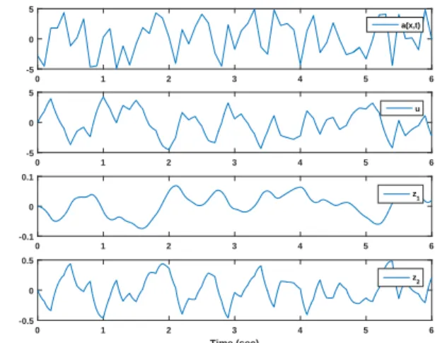
aM, the accuracy of the closed-loop system is low. This is illustrated by Fig. 1: a LSF (5) is applied to system (4) whose initial conditions are z1(0) = z2(0) = 0. The term a(x, t) is taken such that |a(x, t)| ≤ 5 with b(x, t) = 1. Controller gains k1 and k2 are fixed to 32 and 8 respectively. The boundaries obtained for z1 and z2 (i.e. max|z1|, max|z2|) are: |z1| ≤ 7.43 × 10⁻² |z2| ≤ 4.82 × 10⁻¹ (7) 0 1 2 3 4 5 6 -5 0 5 a(x,t) 0 1 2 3 4 5 6 -5 0 5 u 0 1 2 3 4 5 6 -0.1 0 0.1 z 1 0 1 2 3 4 5 6 Time (sec) -0.5 0 0.5 z 2
Fig. 1: LSF From top to bottom: perturbation/uncertainty, control input, z1 and z2 versus time (sec).
In order to improve the accuracy, a control solution is to apply the TWC [7] defined by
u = −k1sign(z1) − k2sign(z2) (8) It has been proven [7] that, if it is well tuned, this controller allows the establishment of a second order sliding mode, i.e. the system trajectories converge in a finite time to the set S defined as
S = {(z1, z2) ∈ Z | z1= z2= 0}. (9) with Z ⊂ R2. In case of a sampled controller with sampling period τ , the trajectories of the system converge in a finite time to the set
Sr= {(z
1, z2) ∈ Z | |z1| ≤ µ1τ2, |z2| ≤ µ2τ } (10) with µ1, µ2 > 0. This behavior of (1) on S (resp. Sr) is called ideal (resp. real) second order sliding mode. The TWC allows the establishment of (ideal or real) second order sliding mode if the gains k1 and k2 are tuned as [7]
k1> k2> 0, (k1− k2)bm> aM, (k1+ k2)bm− aM >(k1− k2)bM+ aM.
(11)
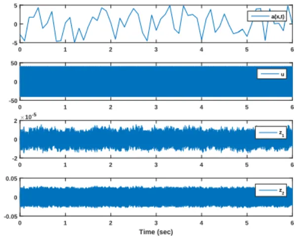
This can be seen in Fig. 2 where a TWC with sampling period 10−4sec is applied to system (4) whose initial con-ditions are z1(0) = z2(0) = 0 in the presence of a perturbation/uncertainty (|a(x, t)| ≤ 5 and b(x, t) = 1) with gains k1 and k2 fixed to 32 and 8 respectively. The boundaries obtained for z1 and z2 are:
|z1| ≤ 1.56 × 10⁻⁵ |z2| ≤ 2.93 × 10⁻²
(12) which is largely more accurate than the LSF.
B. Energy Consumption
Define the energy consumption of both contollers thanks to the following indicator [14]
E = Z t1
t0
0 1 2 3 4 5 6 -5 0 5 a(x,t) 0 1 2 3 4 5 6 -50 0 50 u 0 1 2 3 4 5 6 -2 0 2×10 -5 z 1 0 1 2 3 4 5 6 Time (sec) -0.05 0 0.05 z2
Fig. 2: TWC From top to bottom: perturbation/uncertainty, control input, z1 and z2 versus time (sec).
The energy consumed by the TWC for 2 ≤ t ≤ 6 is 4004.92 and that of the LSF for the same time interval is 13.93. Hence one notices that the energy consumption of the TWC is much greater than that of the LSF.
IV. MAINRESULTS
Based on the two controllers explored above, a new controller is proposed in the sequel that is a trade-off between the LSF and the TWC. The objective is to get a low energy consuming controller with high accuracy.
The proposed controller is written in the form of the con-troller proposed in [3]
u = −k1|z1| α
2−αsign(z1) − k2|z2|αsign(z2), (14)
with k1and k2tuned as in (11) and the time varying exponent gain α ∈ {0, 1} is switching between 0 and 1 thanks to the following law α = ( 1 if |z1| < εz1∧ 1|z 2| < εz2 0 otherwise (15) Parameters εz1and εz2 are positive constants set by the user.
Theorem 1: Consider system (4) under assumptions A1-A4 and controlled by (14)-(15). If k1 and k2are tuned as in (11), then there exist positive parameters εz1 and εz2 such
that the trajectories of system (4) converge, in a finite time, to |z1| ≤ ε2z2 2Kmin M + εz1 |z2| ≤ q ε2 z2+ 2K max m εz1 (16) where Kmmax= bM(k1− k2) + aM, KMmin= bm(k1+ k2) − aM. (17)
Proof: First-of-all, suppose that the trajectory of the sys-tem in the phase plan (z1, z2) is initially outside D: therefore,
1The notation ∧ is used for the logical AND operator.
the TWC is applied. As mentioned in Section III, given that k1 and k2 fulfill (11), the system trajectory converges in a finite time towards the origin (9) [7]. Therefore, it is guaranteed that the system trajectory will converge to D in a finite time (see curve O − P in Fig. 3).
When that occurs, the LSF is applied and consequently the trajectory of the system may potentially leave D due to perturbations/uncertainties. This case can be divided into 4 potential cases
Case 1. the trajectory of the system leaves D through [AB] or [F E];
Case 2. the trajectory of the system leaves D through [CD] or [GH];
Case 3. the trajectory of the system leaves D through [BC] or [F G];
Case 4. the trajectory of the system leaves D through [HA] or [ED].
In the sequel, for each case, the convergence boundaries of z1 and z2 are given.
Case 1. The trajectory of the system cannot leave D crossing [AB] (resp. [F E], see Fig. 3) since the TWC guarantees that
˙
z2< 0 (resp. ˙z2> 0) and therefore z2cannot increase (resp. decrease).
Case 2. Since z2< 0 (resp. z2> 0) along [CD] (resp. [GH], see Fig. 3), then z1 is decreasing (resp. z1 is increasing). Hence, the trajectories of the system cannot leave (D) crossing [CD] (resp. [GH]).
Case 3. Considering the worst case, ˙z2 = −KMmin, it gives the most external trajectory obtained from a point L on [BC] (see L in Fig. 3a) where Kmin
M is the minimal possible variation of z2 in absolute value when the large gain of the TWC is applied. The expression of z1(M ) 2, with z2(M ) = 0, is given by z1(M ) = z22(L) 2Kmin M + εz1 (18)
Therefore, the worst case is when z2(L) is maximal, i.e. point L coincides with B. So, equation (18) becomes
z1(M ) = ε2z2 2Kmin
M
+ εz1 (19)
Then, the trajectory will enter D crossing [CD]. This is proven by calculating z2(N ), with the point N such that z1(N ) = εz1. Considering the worst case, ˙z2 = −K
max m gives the farthest trajectory from the origin, where Kmmax is the maximal variation of z2in absolute value when the small gain of the TWC is applied. The expression of z2(N ) is
z2(N ) = −εz2 s Kmax m Kmin M (20)
From (11), one has K
max m Kmin
M
< 1; therefore, z2(N ) < −εz2.
Hence, the trajectory of the system enters D through [CD].
2With abuse of notation, z
1(M ) is the z1-coordinate of point M . The
Finally, one concludes that if the trajectories of the system leave D through [BC], then
|z1| ≤ ε2z2 2Kmin M + εz1 |z2| ≤ εz2 (21)
and the trajectory reaches again the domain D.
Due to symmetry, the same bounds are obtained if the trajectory leaves D through [F G].
Case 4. Considering the worst case, ˙z2 = Kmmax gives the most external trajectory obtained from a random point Q on [HA] (see Q in Fig. 3b). The expression of z2(R), R being such that z1(R) = 0, is given by
z2(R) = q ε2 z2+ 2K max m z1(Q) (22) Therefore, the worst case is obtained when z1(Q) is maximal and hence point Q coincides with H. So, (22) becomes
z2(R) = q ε2 z2+ 2K max m εz1. (23)
The trajectory will enter D crossing [EF ]. This is proven by calculating z1(S), S being such that z2(S) = εz2.
Considering the worst case, ˙z2= −KMmin gives the farthest trajectory from the origin. The expression of z1(S) reads as
z1(S) = εz1 s Kmax m Kmin M . (24)
From (11), one deduces that z1(S) < εz1. Hence the
trajectory of the system enters D through [AB].
Finally, one concludes that, if the trajectories of the system leave D through [HA] or [ED] (due to symmetry), then
|z1| ≤ εz1 |z2| ≤ q ε2 z2+ 2K max m εz1. (25)
Therefore, by combining the 4 latter cases, the ultimate convergence boundary of the trajectories of the system is
|z1| ≤ ε2 z2 2Kmin M + εz1 |z2| ≤ q ε2 z2+ 2K max m εz1
This concludes the proof.
Remarks and parameter tuning.
- Since the proposed controller switches between the LSF and the TWC (depending on the accuracy of the closed-loop system), the gains k1 and k2 have to be tuned to converge for both algorithms. Hence, the gains should satisfy (11) given that the stability of the closed-loop system with the LSF is ensured if k1, k2> 0 [5].
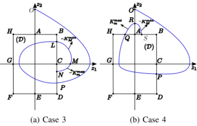
(a) Case 3 (b) Case 4
Fig. 3: Description of the system trajectory in the phase plan (z1, z2).
- If the trajectories of the system are inside D such that D = {(z1, z2) ∈ Z | |z1| < εz1∧ |z2| < εz2} (26)
then the desired accuracy of the system is reached; therefore, the LSF (α = 1) is applied to decrease the energy consumption.
- If the trajectories of the system are outside D, it means that the desired accuracy is not reached probably due to perturbations/uncertainties. Hence, the TWC (α = 0) is applied in order to force the trajectories back to D. - A key point of this new control strategy is that its energy
consumption is less than that of the TWC. Therefore, when the proposed controller behaves as a LSF, its maximal energy consumption should be less than the minimum energy consumption of the TWC. Hence, εz1
and εz2 should satisfy the following condition:
k1εz1+ k2εz2 < k1− k2 (27)
Note that the left side of the inequality is the maximal control effort (in absolute value) of the LSF (knowing that the LSF is only applied in D) and the right side of the inequality is the minimal control effort (in absolute value) of the TWC.
- Note that by a practical point of view, the TWC forces the trajectories to reach Sr (10). It means that, if one wants to get an efficient trade-off, one has to tune εz1
and εz2 such that the boundaries in (16) are greater than
µ1τ2 and µ2τ for z1 and z2 respectively. Otherwise, a risk is to have the TWC all the time. Beyond that, the user can tune εz1 and εz2in a way to obtain the desired
accuracy (i.e. boundaries) following (16).
V. SIMULATIONRESULTS
In this section, simulations are presented and performances of the proposed control algorithm are compared to those of the TWC and the LSF. Simulations have been made using Matlab Simulink with Euler’s method. The sampling period is fixed to 10−4sec. a(x, t) and b(x, t) are considered variable with the following bounds (see Fig. 4)
aM = 5, bm= 0.95, bM = 1.05 (28) In all cases, the gains k1 and k2 are fixed to 32 and 8 respectively verifying (11). The additional parameters for the
proposed controller are firstly: εz1 = 5 × 10 −5, ε z2 = 5 × 10⁻² and then: εz1 = 2 × 10 −5, ε z2 = 2 × 10 −2 with both cases fulfilling condition (27).
The results are shown in Fig. 4 and 5 for the proposed controller, in Fig. 6 for the LSF and in Fig. 7 for the TWC. As seen in Fig. 4 and 5, at t = 0 sec the proposed controller applies α = 0 (TWC) since the trajectory is outside D. When the system converges to D (t ' 1.4 sec), the proposed controller applies the LSF but due to pertur-bations/uncertainties, the trajectory leaves D and therefore the proposed controller applies the TWC again and so on. Hence, as the trajectory is evolving around D, the proposed controller switches between TWC (α = 0) and LSF (α = 1).
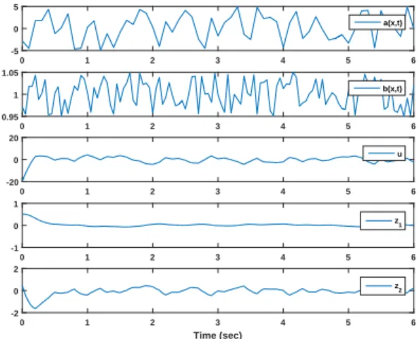
0 1 2 3 4 5 6 -5 0 5 a(x,t) 0 1 2 3 4 5 6 0.95 1 1.05 b(x,t) 0 1 2 3 4 5 6 0 0.5 1 α 0 1 2 3 4 5 6 -50 0 50 u 0 1 2 3 4 5 6 -1 0 1 z1 0 1 2 3 4 5 6 Time (sec) -10 0 10 z 2 2 2.1 2.2 0 0.51 α zoom
Fig. 4: Proposed controller: (from top to bottom) a(x, t), b(x, t), α (with zoom), control input, z1 and z2 versus time (sec) with εz1= 5 × 10 −5and ε z2 = 5 × 10 −2. 0 1 2 3 4 5 6 -5 0 5 a(x,t) 0 1 2 3 4 5 6 0.95 1 1.05 b(x,t) 0 1 2 3 4 5 6 0 0.5 1 α 0 1 2 3 4 5 6 -50 0 50 u 0 1 2 3 4 5 6 -1 0 1 z 1 0 1 2 3 4 5 6 Time (sec) -10 0 10 z2
Fig. 5: Proposed controller: (from top to bottom) a(x, t), b(x, t), α, control input, z1 and z2 versus time (sec) with εz1= 2 × 10
−5and ε
z2 = 2 × 10 −2.
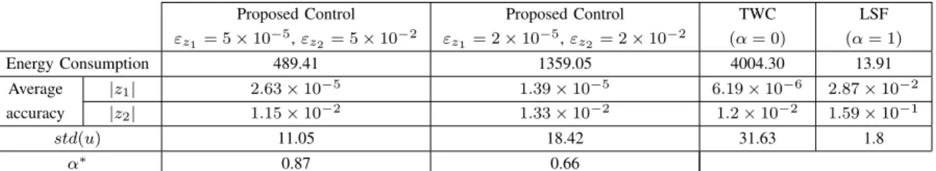
The consumed energy for 2 ≤ t ≤ 6 (steady state) by the proposed controller (Fig. 4, 5 and Table I) is significantly less than the consumed energy with the TWC (Fig. 7).
The average accuracy provided during the same time interval by the proposed controller is significantly better than that of the LSF (Fig. 6) and comparable to that of the TWC. The trade-off is manifested by examining the average accuracy and energy consumption of the proposed controller for different values of εz1 and εz2. It can be seen that for
bigger values of εz1 and εz2 the closed-loop system is less
accurate (on z1) but the energy consumption is less and vice-versa. Therefore, one can either favor accuracy or lower energy consumption by tuning εz1 and εz2 (see Table I).
Note also that when εz1 = 5 × 10
−5 and ε z2 = 5 × 10 −2 (resp. εz1= 2 × 10 −5 and ε z2 = 2 × 10 −2), α∗= 0.87 (resp. 0.66)3 with 2 ≤ t ≤ 6. This means that after the system converges to D for the first time, the LSF is applied 87 % (resp. 66 %) of the time hence the frequency of the chattering with the proposed controller is reduced. The indicator used to quantify this reduction is the standard deviation (std) of the control input u where it can be seen that with the proposed controller it is less than that of the TWC (see Table I).
0 1 2 3 4 5 6 -5 0 5 a(x,t) 0 1 2 3 4 5 6 0.95 1 1.05 b(x,t) 0 1 2 3 4 5 6 -20 0 20 u 0 1 2 3 4 5 6 -1 0 1 z 1 0 1 2 3 4 5 6 Time (sec) -2 0 2 z 2
Fig. 6: LSF: (from top to bottom) a(x, t), b(x, t), control input, z1 and z2 versus time (sec).
0 1 2 3 4 5 6 -5 0 5 a(x,t) 0 1 2 3 4 5 6 0.95 1 1.05 b(x,t) 0 1 2 3 4 5 6 -50 0 50 u 0 1 2 3 4 5 6 -1 0 1 z 1 0 1 2 3 4 5 6 Time (sec) -10 0 10 z 2
Fig. 7: TWC: (from top to bottom) a(x, t), b(x, t), control input, z1 and z2 versus time (sec).
Remark:
Without loss of generality, a special case is taken to show the closeness of the analytical bounds of z1 and z2 found in (16) to the bounds obtained by simulation. No uncertainty on the control input is considered (bm= bM = 1) and a(x, t) is considered maximal and constant such that a(x, t) = aM = 5. The gains k1 and k2 are taken 32 and 8 respectively and εz1 and εz2 are taken 5 × 10
−5 and 5 × 10⁻² respectively.
3α∗ is the mean value of α in the steady state with the proposed
Proposed Control εz1= 5 × 10 −5, ε z2= 5 × 10 −2 Proposed Control εz1= 2 × 10 −5, ε z2= 2 × 10 −2 TWC (α = 0) LSF (α = 1) Energy Consumption 489.41 1359.05 4004.30 13.91 Average accuracy |z1| 2.63 × 10⁻⁵ 1.39 × 10⁻⁵ 6.19 × 10⁻⁶ 2.87 × 10⁻² |z2| 1.15 × 10⁻² 1.33 × 10⁻² 1.2 × 10⁻² 1.59 × 10⁻¹ std(u) 11.05 18.42 31.63 1.8 α∗ 0.87 0.66
TABLE I: Energy consumption, average accuracy on |z1| and |z2|, std(u) and α∗ for the proposed controller, TWC and LSF for 2 ≤ t ≤ 6 (steady state).
When the system converges (i.e. starts evolving around D), its boundaries are:
z1 z2
Analytical bounds 8.57 × 10⁻⁵ 7.35 × 10⁻²
Simulation bounds 6.04 × 10⁻⁵ 2.24 × 10⁻²
TABLE II: Analytical and simulation bounds of z1 and z2. It can be seen from Table II that the analytical and simulation bounds are comparable.
VI. PROSPECTIVE ONα-DYNAMICS
It is possible to consider a dynamic law for α where α varies between 0 and 1. The idea is the following: when the accuracy of the system is low the value of α is decreased dynamically in order to increase the accuracy again. It is important to note that it is sometimes not necessary to have α = 0 to achieve the required accuracy. When the latter is achieved, the value of α is increased in order to decrease the energy consumption.
An example of such an adaptive law is:
˙ α = −1 if β > 0 ∧ α ≥ 1 1 if β < 0 ∧ α ≤ 0 β otherwise , α(0) = 0 β = k(−1 + sign(εZ1− |z1|) + sign(εZ2− |z2|)) (29)
where k, εZ1 and εZ2 are positive constants.
The output of the integrator of ˙α is limited to a minimum value of 0 and a maximum value of 1. By this way, a trade-off between the TWC and LSF is ensured; as a consequence, the gains k1 and k2 have to be tuned to ensure the stability of the closed-loop system ∀α ∈ [0, 1] fixed. Hence, the gains should satisfy (11) (note that exponential stability of the closed-loop system with the LSF is ensured if the gains are positive [5], that is a condition guaranteed by (11)). At t = 0 sec, α = 0: the TWC is applied to ensure the convergence of the system trajectories to B such that
B = {(z1, z2) ∈ Z | |z1| ≤ εZ1∧ |z2| ≤ εZ2} (30)
˙
α is an image of the accuracy of the system: if (z1, z2) ∈ B, it means that desired accuracy is reached. Then, ˙α = k: α increases towards 1 to reduce the energy consumption. If z1 or z2 is outside ]−εZ1, εZ1[ or ]−εZ2, εZ2[ respectively, it
means that desired accuracy is not reached, hence ˙α = −k: α decreases towards zero in order to increase the accuracy.
If both variables are outside of their respective intervals then the rate by which α decreases towards zero is three times faster ( ˙α = −3k) to increase the accuracy faster.
VII. CONCLUSION
A new controller was developed in this paper combining advantages of the LSF and TWC. Low-energy consuming and high accuracy motions of these controllers are taken into account by switching the exponent gain of the proposed controller between 0 (TWC) and 1 (LSF). Simulation results manifest the effectiveness of the proposed controller. Future works will be dedicated to vary α dynamically between 0 and 1 via different adaptive laws with an estimation of the domain of convergence.
REFERENCES
[1] G. Bartolini, A. Levant, A. Pisano, and E. Usai. “Higher-order sliding modes for the output-feedback control of nonlinear uncertain systems.” Variable structure systems: towards the 21st century. Springer, Berlin, Heidelberg (2002): 83-108.
[2] E. Bernuau, D. Efimov, W. Perruquetti and A. Polyakov. “On homo-geneity and its application in sliding mode control.” Journal of the Franklin Institute 351.4 (2014): 1866-1901.
[3] S.P. Bhat and D.S. Bernstein. “Finite-time stability of homogeneous systems.” In proceedings of the American Control Conference, Albu-querque, NM, USA (1997).
[4] C. Edwards and Y. Shtessel. “Adaptive continuous higher order sliding mode control.” Automatica 65 (2016): 183-190.
[5] M. Gopal. Control systems: principles and design. Tata McGraw-Hill Education (2002).
[6] S. Laghrouche, F. Plestan and A. Glumineau. “Higher order sliding mode control based on integral sliding mode.” Automatica 43.3 (2007): 531-537.
[7] A. Levant. “Sliding order and sliding accuracy in sliding mode control.” International journal of control 58.6 (1993): 1247-1263. [8] A. Levant. “Universal single-input-single-output (SISO) sliding-mode
controllers with finite-time convergence.” IEEE transactions on Auto-matic Control 46.9 (2001): 1447-1451.
[9] A. Levant. “Homogeneity approach to high-order sliding mode de-sign.” Automatica 41.5 (2005): 823-830.
[10] F. Plestan, Y. Shtessel, V. Bregeault and A. Poznyak. “New method-ologies for adaptive sliding mode control.” International journal of control 83.9 (2010): 1907-1919.
[11] Y. Shtessel, C. Edwards, L. Fridman and A. Levant. Sliding mode control and observation. New York, NY, USA: Birkhuser (2014). [12] Y. Shtessel, J.A. Moreno, F. Plestan, L.M. Fridman and A.S. Poznyak.
“Super-twisting adaptive sliding mode control: A Lyapunov design.” In proceedings of the IEEE Conference on Decision and Control, Atlanta, GA, USA (2010).
[13] Y. Shtessel, J.A. Moreno, and L. Fridman. “Twisting sliding mode con-trol with adaptation: Lyapunov design, methodology and application.” Automatica 75 (2017): 229-235.
[14] V. Tzoumas, M. A. Rahimian, G. J. Pappas and A. Jadbabaie ”Minimal actuator placement with optimal control constraints.” In proceedings of the IEEE American Control Conference, Chicago, IL, USA (2015) [15] V.I. Utkin. Sliding modes in control and optimization. Springer