HAL Id: hal-01823187
https://hal.archives-ouvertes.fr/hal-01823187
Submitted on 25 Jun 2018HAL is a multi-disciplinary open access
archive for the deposit and dissemination of sci-entific research documents, whether they are pub-lished or not. The documents may come from
L’archive ouverte pluridisciplinaire HAL, est destinée au dépôt et à la diffusion de documents scientifiques de niveau recherche, publiés ou non, émanant des établissements d’enseignement et de
Multiphase model for transformation induced plasticity
Extended Leblond’s model
Daniel Weisz-Patrault
To cite this version:
Daniel Weisz-Patrault. Multiphase model for transformation induced plasticity Extended Leblond’s model. Journal of the Mechanics and Physics of Solids, Elsevier, 2017. �hal-01823187�
Multiphase model for transformation induced plasticity
Extended Leblond’s model
Daniel Weisz-Patrault
LMS, ´Ecole Polytechnique, CNRS, Universit´e Paris-Saclay, 91128 Palaiseau, France
Abstract
Transformation induced plasticity (TRIP) classically refers to plastic strains observed during phase transitions that occur under mechanical loads (that can be lower than the yield stress). A theoretical approach based on homogenization is proposed to deal with multiphase changes and to extend the validity of the well known and widely used model proposed by Leblond, J.-B., De-vaux, J., and DeDe-vaux, J. (1989). Mathematical modelling of transformation plasticity in steels i: case of ideal-plastic phases. International journal of plasticity, 5(6):551–572. The approach is similar, but several product phases are considered instead of one and several assumptions have been released. Thus, besides the generalization for several phases, one can mention three main improvements in the calculation of the local equivalent plastic strain: the deviatoric part of the phase transformation is taken into account, both parent and product phases are elastic-plastic with linear isotropic hardening and the applied stress is considered. Results show that classical issues of singularities arising in the Leblond’s model (corrected by ad hoc numerical functions or thresholding) are solved in this contribution excepted when the applied equivalent stress reaches the yield stress. Indeed, in this situation the parent phase is entirely plastic as soon as the phase transformation begins and the same singularity as in the Leblond’s model arises. A physical explanation of the cutoff function is introduced in order to regularize the singularity. Furthermore, experiments extracted from the literature dealing with multiphase transitions and multiaxial loads are compared with the original Leblond’s model and the proposed extended version. For the extended version, very good agreement is observed without any fitting pro-cedures (i.e., material parameters are extracted from other dedicated experiments) and for the original version results are more qualitative.
Keywords: Transformation plasticity, Super-plasticity, Homogenization
Table 1: Nomenclature
N Number of phase
σk Local stress tensor in the k-th phase
sk Local stress deviator in the k-th phase εk Local strain tensor in the k-th phase
λk, µk Lam´e’s coefficients in the k-th phase
V Representative volume element (RVE)
Vk Volume occupied by the k-th phase in the RVE
Σ Macroscopic stress tensor
S Macroscopic stress deviator
E Macroscopic strain tensor
Et p Transformation induced plastic strain tensor
EcpT Classical plastic strain tensor due to temperature variation
EcpΣ Classical plastic strain tensor due to stress variation Σk Average stress tensor in the k-th phase
Sk Average stress deviator in the k-th phase
1. Introduction
When phase transformations occur under applied mechanical loads that can be much lower than the yield stress, significant plastic strains are observed. This phenomenon called transfor-mation induced plasticity or sometimes super-plasticity received particular attention since the eighties because of numerous applications in mechanical engineering. For instance welding or sheet metal manufacturing (especially the run out process that consists in cooling down a sheet under tension) cannot be approached without considering transformation plasticity. Two different mechanisms have been proposed to explain transformation plasticity by Greenwood and Johnson (1965) and Magee and Paxton (1966). One of the most fruitful model has been proposed by Leblond et al. (1986a) and relies on an homogenization procedure without adding a priori contributions in the plastic strain tensor that would be proportional to phase propor-tion rate. This classic contribupropor-tion results directly from the homogenizapropor-tion procedure itself and both Greenwood and Johnson and Magee mechanisms are thus identified in the obtained contributions. In order to give a more specific and usable form to the homogenized model, a morphological assumption which consists in an idealization of the microstructure has been pro-posed and solved analytically by Leblond et al. (1986b, 1989) without considering hardening effects and by Leblond (1989) if hardening is taken into account. These four papers form the base of the Leblond’s transformation induced plasticity model. Because of its solid theoretical basis and simple explicit formulas for the overall plastic strain increment, Leblond’s model has been intensively used for various engineering applications and has been included (see Bergheau and Leblond (1991)) in a commercial Finite Element software SYSWELD® (2012) dedicated to welding applications. Among many contributions, one can mention for instance quite re-cent applications of the Leblond’s model to welding proposed by Bate et al. (2009); Xu et al. (2012) and sheet metal manufacturing by Lee et al. (2009). Moreover, Kim et al. (2005) devel-oped a numerical implementation of Leblond’s model within the framework of multiplicative elastic-plasticity considering welding applications.
It should be mentioned that several other theoretical strategies to model transformation induced plasticity have also been proposed. For instance Diani et al. (1995) deal with the the-oretical justification of the proportionality of the transformation plastic strain rate, the phase proportion rate and the macroscopic stress deviator. The idea is to consider the complete trans-formation from the reorganization of the crystal lattice. Indeed most authors consider only the hydrostatic part of the phase transformation (considering only the density mismatch between phases), however a very large deviatoric strain also occur during the phase transformation. Di-ani et al. (1995) practically consider the Bain transformation. Fischer et al. (1998) pointed out
the fact that the Leblond’s model neglects shear (i.e., the deviatoric part of the phase transforma-tion) and proposed a formulation of transformation induced plasticity based on thermodynamic considerations. A similar approach which deals with finite strain (multiplicative formalism) has been proposed by Hallberg et al. (2007). These models account for the complete phase transformation tensor but do not enable to derive a simple analytic form for the overall trans-formation plastic strain rate. On the other hand, numerical investigations have been published, for instance Mahnken et al. (2009) proposed a numerical homogenization based on Finite El-ement simulations of random cubic unit cells. Barbe et al. (2007) proposed a Finite ElEl-ement modeling of a unit cell that undergoes a diffusive phase transformation, which is modeled by changing material properties as the transformation goes on. Otsuka (2014) proposed a micro-mechanical model of crystalline plasticity relying on Fast Fourier Transform and periodic cells. Moreover multiphase situations already have been studied in the field of TRIP assisted steels. For instance, Finite Element strategies were used by Van Rompaey et al. (2006) in order to analyze the micromechanics of a transforming inclusion in TRIP assisted steels. Experimental counter-parts have also been published by Lacroix et al. (2008) in order to analyze the effects of transformation kinetics. A mean field homogenization approach was also developed by Delan-nay et al. (2007, 2008) based on a uniform stress/strain approximation per phase. Recent efforts were also published on the transformation in a multiphase steel by Srivastava et al. (2015).
Many authors proposed experimental investigations of transformation induced plasticity and compared results to the Leblond’s model. For instance Taleb et al. (2001) developed an experimental setup to measure transformation induced plasticity in steels. Coret et al. (2002, 2004) developed a tension-torsion testing machine that enables to study transformation induced plasticity under multiaxial loads. Results show that Leblond’s model is qualitatively correct but some quantitative discrepancies between theoretical predictions and measurements are notice-able even though it is the model which describes the more accurately the phenomenon among the tested models.
The original Leblond’s modeling leads to a singularity of the transformation plastic strain increment when the phase proportion of the product phase vanishes. The difficulty is overcome by introducing an ad hoc cutoff function when the product phase proportion tends to zero. Taleb and Sidoroff (2003) proposed an analytic from of this cutoff function by coupling an elastic-plastic parent phase and an elastic product phase (much harder). The singularity disappears since a threshold naturally arises and corresponds to the possibility for the matrix to be entirely elastic. The obtained threshold is very similar to the numerical ad hoc threshold 0.03 introduced in the Leblond’s model. Experimental results are therefore similar. It should be noted that Taleb and Sidoroff (2003) do not modify the global homogenization scheme developed by Leblond et al. (1986a). Furthermore, Petit-Grostabussiat et al. (2004) proposed an experimental counter-part of the Leblond’s model with respect to the possible recovery of strain hardening on the one hand and the classical plasticity due to thermal variations on the other hand. However, other tests performed by Taleb and Petit (2006) show that predictions of the Leblond’s model are not qualitatively correct when pre-hardening (significantly higher than the yield stress of the soft phase) is applied to the test piece before starting the phase transformation. For instance, even for zero macroscopic applied stress, non negligible transformation induced plasticity is observed. This deserves a comment since it is the only situation where the Leblond’s model is not qualitatively correct. Despite the fact that authors present this result as an effect of hardening, this may be rather explained by residual stress issues. Indeed, there is a significant irreversible plastic strain in the parent phase when the phase transformation begins. However
the produced phase is not subjected to this initial plastic strain due to the rearrangement of the crystal lattice, therefore an elastic strain is needed in both parent and product phases to accommodate this geometrical mismatch. This leads to residual stresses whose global average is obviously zero. Since the transformation induced plastic strain rate proposed by Leblond is proportional to the global average deviatoric stress, zero transformation induced plasticity is predicted, in disagreement with experiments proposed by Taleb and Petit (2006). In this contribution, average stresses per phase are used instead of a global average stress, so that residual stress issues may be considered.
It should be noted that Delannay et al. (2007) used an approach relying on average stress per phase and classical Eshelby inclusion problem with tangent stiffness so that plasticity is accounted for. It is concluded that local stress gradients in the parent phase near the trans-formation zone may introduce some discrepancy with a local Finite Element computation for certain size of inclusion. However in this paper, despite the fact that stresses are averaged in each phase, one accounts for stress gradients and therefore local plasticity in the parent phase near the inclusions, by considering an idealized microstructure presented in Appendix A.
Even though the paper is presented with a very general point of view, it is mainly intended for crystalline cubic structures such as steel. It is an attempt to contribute in improving not only the transformation induced plasticity but also the interactions with classical plasticity. Further-more the homogenization scheme is slightly improved by releasing some assumptions made by Leblond et al. (1986a), even though the obtained transformation induced plastic strain is still proportional to the applied stress as in the original Leblond’s model. However, a nonlinear ef-fect has been evidenced in micromechanical Finite Element simulations performed for instance by Leblond et al. (1989). The transformation induced plastic strain rate increases more quadrat-ically than linearly with the stress, once the overall von Mises stress exceeds about half of the yield stress of the parent phase. Therefore this paper is limited to rather low applied stresses. Although relying on the same scheme, the present paper introduces the following details in comparison with the Leblond’s model and Taleb and Sidoroff (2003), where the last three are the most significant with respect to numerical results:
1) Several product phases are considered.
2) Elastic-plastic behavior is considered for both parent and product phases, which regularizes the singularity obtained by Leblond et al. (1986b) for the classical plastic strain rate due to a variation of equivalent stress. This singularity was due to the product phase proportion ap-pearing at the denominator. Leblond et al. (1986b) proposed a numerical function obtained by Finite Element simulations in order to smooth the singularity.
3) The average stress deviator in the parent phase is not equated to the macroscopic stress deviator as it is done by Leblond et al. (1989). This enables to be consistent with the fact that one phase may have a yield stress lower than the others and does not necessarily sustain the macroscopic stress deviator. On the other hand this enables to take into account residual stress issues as in the experiments proposed by Taleb and Petit (2006).
4) The applied macroscopic stress is taken into account as a pre-stress in the calculation of the equivalent plastic strain, which is neglected by Leblond et al. (1989) and Taleb and Sidoroff (2003).
5) The deviatoric part of the phase transformation has been taken into account through a sim-plified analytic calculation.
consider elasticity in the parent phase. However, this is true only without applied stress. Indeed if an equivalent stress equal to the yield stress is applied to the parent phase the latter would be entirely plastic as soon as the phase transformation begins, which leads to the same singularity obtained by Leblond et al. (1989) when the product phase proportion vanishes. Leblond et al. (1989) applied a cutoff function to smooth the singularity. It should be mentioned that the singularity problem arises only for the transformation induced plasticity and not for the classical plasticity due to temperature changes although both problems are very similar. That is why, in this paper this technical issue is solved by considering that nucleation of the product phase is discontinuous, that is to say that a minimal finite volume of product phase is created when a lower total energy state can be reached by rearranging the atomic lattice in this volume as suggested by Bluth´e et al. (2016) and in agreement with Delannay et al. (2008). Therefore when there is no product phase (pure matrix of parent phase), one cannot consider an incremental variation of the product phase proportion, one should directly consider a finite size for the inclusion. This amounts to introduce a cutoff function as Leblond et al. (1989) did, where the threshold is determined by the minimal size that can nucleate. However, the nucleation of an inclusion of finite size is responsible for plastic strains that can be taken into account by setting an initial value for the transformation induced plastic strain corresponding to the plastic strain resulting from the nucleation of the inclusion.
2. Homogenization: general scheme
In the whole paper, phase proportions and temperature evolutions are considered as known external quantities evaluated from a thermo-metallurgical model or measurements. The follow-ing calculations are identical to those presented by Leblond et al. (1986a) excepted that sums over several phases are required. At the local scale the total strainε is written as follows:
ε = εe + εthm+ εp (1)
where εe is the elastic strain, εp the plastic strain, εthm the thermo-metallurgical strain that
includes both the classic thermal expansion due to temperature changes and the phase transfor-mation due to the rearrangement of the crystal lattice (classic orientation models such as Bain, Nishiyama-Wasserman or Kurdjumov-Sachs can be used). As mentioned in the introduction, εthm is decomposed into hydrostatic and deviatoric parts, that are dealt with separately.
εthm = εthm,h+ εthm,d (2)
whereεthm,d = εthm− tr(εthm)1/3 and εthm,his the volume variation due to temperature changes
and phase transitions. The homogenization procedure consists in averaging total strain and stress tensors over the volume of the RVE denoted by V.
E=⟨ε⟩
V and Σ =
⟨
σ⟩V (3)
Leblond et al. (1986a) assumed that the homogenized compliance tensor could be equated to the local compliance tensor in the calculation of⟨εe⟩
V which amounts to assume to neglect the
effect of the influence tensor, which leads to:
Ee =⟨εe⟩
Therefore the macroscopic thermo-metallurgical reads:
Ethm =⟨εthm⟩
V (5)
and the macroscopic plastic strain reads:
Ep =⟨εp⟩
V (6)
First, a simple formula is derived for the thermo-metallurgical strain rate ˙Ethm. The deviatoric part of the phase transformation is written along the crystallographic directions. In this contri-bution it is assumed that inclusions of product phases are isotropically orientated in the RVE. If no average stress is applied one obtains:
⟨ εthm,d⟩
V = 0 (7)
If a macroscopic stress is applied, one can consider texturation, that is to say that the applied stress can have an impact on the orientation distribution of product phase inclusions. However this effect is neglected in this contribution since relatively low applied stress is considered, and (7) is assumed to hold even with macroscopic stress. On the other hand, the hydrostatic part εthm,h is constant in each inclusion, hence the following mixture rule:
Ethm = 1 − N ∑ k=2 Xk εthm1 ,h+ N ∑ k=2 Xkεthmk ,h (8)
The time derivative is thus: ˙ Ethm = N ∑ k=2 ( εthm,h k − ε thm,h 1 ) ˙ Xk+ 1 − N ∑ k=2 Xk ˙εthm1 ,h+ N ∑ k=2 Xkε˙thmk ,h (9)
At the first order, the term εthmk ,h − εthm1 ,h may be identified as the volume variation due to the phase transition only. Thus, if a mass Mk of phase 1 is transformed into phase k, the volume
variation is (1/3) (ρ1(T )/ρk(T )− 1). Moreover, by definition of thermal expansion coefficients
˙ εthm,h k = αkT , hence:˙ ˙ Ethm = N ∑ k=2 1 3 ( ρ1(T ) ρk(T ) − 1 ) ˙ Xk+ α1+ N ∑ k=2 Xk(αk− α1) ˙T (10)
The main objective of the present paper is to derive a simple formulation for ˙Epas a function of the homogenized known quantities, that are the macroscopic applied stress, temperature and phase proportions in addition to material parameters. A direct derivation of (6) gives:
˙ Ep = 1 V N ∑ k=1 d dt [∫ Vk εp kdVk ] (11)
where Vk denotes the volume of the k-th phase. ConsiderVkthe speed of the front∂Vk and nk
with other phases. Since V = ∪Nk=1Vk and∂V1 = ∪Nk=2∂Vk and n1(x) = −nk(x) (for x ∈ ∂Vk) one obtains: ˙ Ep = N ∑ k=1 1 V ∫ Vk ˙ εp kdVk+ N ∑ k=2 1 V ∫ ∂Vk ( εp k − ε p 1 ) (Vk· nk) dSk (12) Hence: ˙ Ep= N ∑ k=1 Xk ⟨ ˙ εp k ⟩ Vk + N ∑ k=2 ⟨ εp k − ε p 1 ⟩ Vk·nk ˙ Xk (13) where: ⟨ εp k − ε p 1 ⟩ Vk·nk = ∫ ∂Vk ( εp k − ε p 1 ) (Vk· nk) dSk ∫ ∂Vk(Vk· nk) dSk (14) Leblond et al. (1986a) assumed a dependence between the plastic strain rate in each phase and sort of macroscopic state variables such as temperature T , stressΣ and phase proportions
X2, · · · , XN (it should be noted that X1is not independent of all the other phase proportions and
should be discarded): ˙ εp k = δεp k δΣ : ˙Σ + δεp k δT T˙ + N ∑ m=2 δεp k δXm ˙ Xm (15) Therefore: ˙
Ep = ˙EcpΣ + ˙EcpT + ˙Et p (16) where: ˙ EcpΣ = N ∑ k=1 Xk ⟨δεp k δΣ ⟩ Vk : ˙Σ ˙ EcpT = N ∑ k=1 Xk ⟨δεp k δT ⟩ Vk ˙ T ˙ Et p = N ∑ k=1 N ∑ m=2 Xk ⟨ δεp k δXm ⟩ Vk ˙ Xm+ ⟨ εp k − ε p 1 ⟩ Vk·nk ˙ Xk (17)
As detailed by Leblond et al. (1986a), the first term of ˙Et p corresponds to the Greenwood and Johnson mechanism and the second term to the Magee mechanism.Indeed, the Greenwood and Johnson’s mechanism is related to plasticity in the whole volume of the weaker phase and should arise as a volume integral. While the Magee’s mechanism is related to the plastic strain variation of a given point undergoing a phase transformation and should arise as a surface inte-gral over the phase transition front. Following the idea of Leblond et al. (1989), it is assumed that the Magee’s mechanism is negligible.
The stress tensor in the k-th phase is denoted by σk and its deviator is denoted by sk. The von Mises equivalent stress is denoted byσeqk = √(3/2)sk : sk and the equivalent plastic strain rate (or cumulative plastic strain rate) is denoted by ˙εeqk =
√
(2/3)˙εkp: ˙εkp. The von Mises flow rule reads: ˙ εp k = 3 ˙εeqk 2σYk sk (18)
It is assumed that one can replace the local stress deviator sk by its volume average Sk =⟨sk⟩
Vk , which corresponds for instance to the assumption of constant fields per phase. However it is
not assumed that the average stress deviator in the k-th phase can be equated to the average stress deviator in the RVE as proposed by Leblond et al. (1986b). Hence:
˙ EcpΣ = N ∑ k=1 3Xk 2σY k Sk⟨δε eq k δΣ ⟩ Vk : ˙Σ ˙ EcpT = N ∑ k=1 3Xk 2σY k Sk⟨δε eq k δT ⟩ Vk ˙ T ˙ Et p = N ∑ k=1 N ∑ m=2 3XkSk 2σYk ⟨δεeq k δXm ⟩ Vk ˙ Xm (19)
3. Classical plasticity due to stress variations
This section deals with the term ˙EcpΣ in (19) when between t and t+δt the macroscopic stress varies fromΣ to Σ + δΣ. Leblond et al. (1986b) assumed that the parent phase is purely plastic and the product phase purely elastic. This assumption is released in the present contribution and elatic-plastic behavior with linear hardening is considered for all phases. The idealized microstructure is similar to those proposed by Leblond et al. (1986b), that is to say parallel bars with sections proportional to the phase proportions as shown in figure 1.
Figure 1: Idealization of applied stress
Following the idea proposed by Leblond et al. (1986b) it is assumed that ˙EcpΣ is non-zero only if there is a variation of the equivalent von Mises stress Σeq = √(3/2)Σ : Σ. Thus (19)
becomes: ˙ EcpΣ = N ∑ k=1 3Xk 2σY k Sk⟨ δε eq k δΣeq ⟩ Vk ˙ Σeq (20)
From the simple idealization presented in figure 1 it is inferred: δΣeq = N ∑ k=1 XkδΣ eq k (21)
The following simple uni-dimensional elastic-plastic model is used. δΣeq k = Ekδε if δΣeq < 0 or Σ eq k < σ Y k(ε eq k ) γkσYk0δε if Σ eq k = σ Y k(ε eq k ) andδΣ eq ≥ 0 (22)
with the following linear hardening rule: σY k(ε eq k )= σ Y0 k ( 1+ γkε eq k ) (23) where γk is a hardening parameter and σYk0 the initial yield stress (before any hardening). It
should be noted that it is considered thatδΣeqandδΣeqk have the same sign in (22). By combining (22) and (21) and denoting E and P the sets of indexes verifying the first and the second conditions in (22) respectively, one obtains:
δε = δΣeeq E and δΣ eq k = e EkδΣeq e E (24) where: e E =∑ l∈E XlEl+ ∑ m∈P XmγmσYm0 e Ek = { Ek if k∈ E γkσYk0 if k∈ P (25)
By analogy with (24) one assumes that: ˙ Σk = e EkΣ˙ e E (26)
Therefore the deviatoric stress Sk is evaluated from the initial value by adding at each time in-crement the deviatoric part of (26). This approach enables to take into account residual stresses whose global average is zero although average stresses in each phase may be significant.
The evaluation of conditions E and P is up-dated at each time increment using (24) and (23). It is clear that the strain increment (24) is elastic when k ∈ E and plastic when k ∈ P. Eventually, the classic plastic strain increment due to stress variations is obtained:
⟨ δεeq k δΣeq ⟩ Vk = 01 if k ∈ E e E if k ∈ P and E˙cpΣ = 0 if Σ˙eq < 0 ∑ k∈P 3Xk 2σY k Sk e E ˙ Σeq if Σ˙eq ≥ 0 (27)
The classic plastic strain increment due to a variation of applied stress given in (27) is clearly not singular when X1 → 0 or 1 because eE at the denominator cannot vanish. This overcomes
the difficulty that arose in the work of Leblond et al. (1986b) when no hardening was taken into account (an ad hoc function obtained from Finite Element simulations was introduced by Leblond et al. (1986b) in order to smooth the singularity).
4. Transformation induced plasticity
This section deals with the term ˙Et pin (19) when between t and t+ δt the phase proportions vary from Xmto Xm+ δXm.
The calculation of the equivalent plastic strain variation is divided into two parts. The inclusion is first subjected to the deviatoric part of the phase transformation, then the hydrostatic parteεthm1. That is to say that the loading path is imposed. This approach is obviously not
rigorous since plasticity is considered. However, an approximate estimation can be obtained. The proposed loading path may seem arbitrary, however it leads to a very simple analytic solution. Therefore one can write:
δεeq k = δε eq,d k + δε eq,h k (28)
where superscripts d and h refer to the contributions due to deviatoric and hydrostatic parts of the phase transformation respectively. For the hydrostatic part, fields in the inclusion are hydrostatic and do not contribute to additional plastic strain in the inclusion, thus:
δεeq,h
k = 0 if k , 1 (29)
Furthermore, the deviatoric part of the phase transformation being very intense, shear levels in the inclusions cannot be sustained. Therefore plastic deformations take place in all inclu-sions. The matrix may also undergo plastic deformation, however this contribution is neglected because it is very localized near the inclusion, thus one has:
δεeq,d
1 = 0 (30)
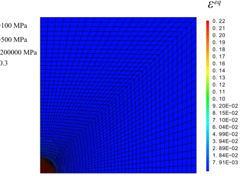
The latter assumption may seem incorrect since the matrix of parent phase may be much softer than the inclusion of product phase. However, the inclusion is subjected to a very large purely deviatoric eigenstrain, thus it is sufficient that the matrix does not allow for the inclusion to move freely so that the inclusion is entirely plastic. A Finite Element simulation using Castem (CEA (2011)) is proposed in figure 2. The imposed eigenstrain is obtained from the classical Bain oritentation model (33) and the inclusion concentrates most of plastic strain even though the inclusion yield stress is five times larger than the matrix yield stress.
Furthermore, each product phase is assumed to have no influence on other product phases, hence: ⟨δεeq,d k δXm ⟩ Vk = 0 if k , m (31) Eventually (19) reads: ˙ Et p = N ∑ k=2 3XkSk 2σY k ⟨δεeq,d k δXk ⟩ Vk ˙ Xk+ 3X1S1 2σY 1 N ∑ m=2 ⟨δεeq,h 1 δXm ⟩ V1 ˙ Xm (32) 4.1. Deviatoric part
For steel, the deviatoric part of the phase transformation is very large in comparison with the hydrostatic part, and very large local plastic deformations occur. However, unlike the hy-drostatic part, the deviatoric part depends on the local lattice directions of each inclusion un-dergoing an increment of phase transition. Since each phase in the RVE is made of several inclusions isotropically orientated, both the deviatoric imposed eigenstrain and the associated plastic strain tend to compensate from one inclusion to another. This is clear for isotropic poly-crystalline configurations, but also for mono-crystals considering the cubic symmetry of the phase transformation related to Bain orientation model for instance. Indeed, if eX, eY, eZdenote
the lattice directions of the mono-crystal the deviatoric part of the eigenstrain due to the phase transition is:
εdev
B = εB(eX ⊗ eX+ eY ⊗ eY− 2eZ⊗ eZ) (33)
where B means Bain and whereεB ≃ 11 %. It is clear that in the mono-crystal all inclusions
have the same lattice directions up to a permutation (i.e., one can haveεdev
B = εB(eY⊗ eY+ eZ⊗
eZ− 2eX⊗ eX) orεdevB = εB(eX⊗ eX+ eZ⊗ eZ− 2eY⊗ eY)). Thus the average is obviously zero if
directions are identically distributed. This compensation effect explains the fact that there is no deviatoric strain at the macroscopic scale for a free dilatometric test, only the hydrostatic part of the phase transformation has a non vanishing average (10).
However, since an average stress is applied to the RVE, the average plastic strain does not completely vanish in spite of compensations due to the isotropic distribution. Indeed, the ap-plied stress is involved in the von Mises yield criterion and globally modifies plastic strain tensors. Moreover one can consider texturation, that is to say that the applied stress may also modify inclusion orientations and favor some directions so that the overall orientation distribu-tion of the eigenstrain due to the phase transformadistribu-tion is not isotropic anymore. This texturadistribu-tion effect is neglected in this contribution since the applied stress level is relatively low.
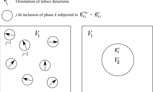
Since the equivalent plastic strain rate involved in (32) does not compensate from one in-clusion to another, (32) should not be applied directly to each inin-clusion. This difficulty may be overcome by considering Nk inclusions indexed by j of the k-th phase with isotropic
distribu-tion and by directly adding all deviatoric eigenstrain tensors due to the phase transidistribu-tion denoted byε∗,dk, j and all plastic strain tensors denoted byεkp, j. Thus the average is given by:
εp k = 1 Nk Nk ∑ j=1 εp k, j 1 Nk Nk ∑ j=1 ε∗,d k, j = 0 (34)
However the problem of each inclusion j with a general global applied stress and subjected to a known local deviatoric eigenstrain ε∗,dj and an unknown local plastic strain εkp, j is not easily solved (where local refer to the crystallographic coordinate system). Thus, another simpler ap-proach is proposed in this paper and consists in constructing an average inclusion that gathers all inclusions of the product phase k and accounts for the isotropic orientation problem. The non-vanishing part of the average plastic strain denoted byεkpis determined by considering an infinite matrix containing a spherical inclusion subjected only toεkp (since the average devia-toric part of the phase transformation has been neglected because texturation is not taken into account), as shown in figure 3.
Figure 3: Schematic problem for the deviatoric part of phase trnasformation
Then the classic solution obtained by Eshelby (1957) is used:
sk = −µkξkεkp (35) where: ξk = 2µ1(9λ1+ 14µ1) λ1(9µ1+ 6µk)+ 2µ1(7µ1+ 8µk) (36) The unknown tensor εkp is then determined by verifying the von Mises yield criterion in the
average inclusion. √
3
2(sk + Sk) : (sk+ Sk)= σ Y
k (37)
Since the average plastic strain is due to the average stress, one can assume that Sk = βkεkp
hence: |βk| = 2 3 Σeq k εeq,d k (38) Thus (37) becomes: 3 |β − µ ξ| εeq,d = σY (39)
Hence: εeq,d k = 2 3 σY k − Σ eq k µkξk (40) And: δεeq,dk = 0 in Vk 2 3 σY k − Σ eq k µkξk inδVk (41) Eventually one obtains:
⟨δεeq,d k δXk ⟩ Vk = 1 Xk 2 3 σY k − Σ eq k µkξk (42) 4.2. Hydrostatic part
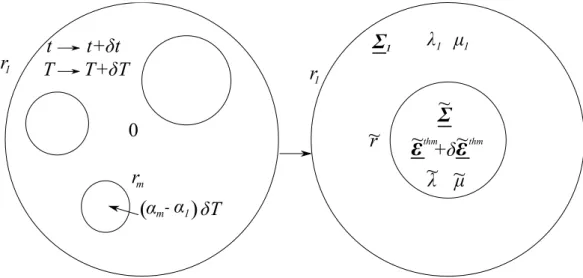
For the hydrostatic part, the equivalent plastic strain increment is also evaluated by con-sidering an idealization of the microstructure. In this section, the parent phase is considered as a bounded hollow spherical matrix in which a spherical inclusion represents all the product phases (index k= 2, · · · , N) gathered into one, as described on the right of figure 4. This choice may seem arbitrary but it is not more arbitrary than the usual choice on the left of figure 4 and it enables to keep the same ideas as Leblond et al. (1989). This modeling choice also ensures a total continuity with the classic bi-phase situation and can therefore be easily compared to other models. The inclusion composed of all the product phases has a radius such as the volume of the inclusion matches the total volume of the product phases, thus:
er = N ∑ k=2 r3k 1 3 (43)
Figure 4: Phase transition
The stress eΣ applied in the inclusion is obtained by considering that each product phase has a constant applied stressΣk. Thus, paying attention to the fact that the average is done only on
the volume occupied by the product phases V−V1(that is why 1− X1arises at the denominator) one obtains: eΣ =∑N k=2 Xk 1− X1 Σk (44)
By analogy with section 3 one obtains the average material properties: eλ =∑N k=2 Xk 1− X1 λk and eµ = N ∑ k=2 Xk 1− X1 µk and eα = N ∑ k=2 Xk 1− X1 (αk − α1) (45)
For each time step, plastic increments depend on the whole local stress and strain history be-cause of non-linearity. Obviously this information is too much detailed and a compromise should be found. In this paper, for each time step, the local stress and strain history is ap-proximated by applying first the stress tensors eΣ and Σ1 (considered as pre-stresses) and the hydrostatic eigenstraineεthm that represents the overall hydrostatic part of the phase transfor-mation and thermal expansion averaged in the inclusion constituted of all the product phases. Then, from this initial state, the plastic increment is calculated by applying temperature and phase proportion variations. It should be noted that Leblond et al. (1989) do not take this as-pect into account because neither the macroscopic stress nor the hydrostatic eigenstrain in the product phase is considered in the calculation of the equivalent plastic strain increment, only the eigenstrain due to the variation of temperature or phase proportion is taken into account. Taleb and Sidoroff (2003) implicitly consider the local stress and strain history due to the eigenstrain related to the phase transformation by first applying the eigenstrain in the inclusion and then applying the phase proportion increment, however the applied stress is not taken into account.
When the temperature varies from the initial temperature Tini to the actual temperature T ,
thermal expansion can be seen as a homogenous thermal expansion with coefficient α1 in the
whole RVE and then a thermal expansion in the product phases with coefficients αk− α1. The
first homogenous thermal expansion does not generate plastic strain and can be discarded in the eigenstrain to apply to the inclusion. Considering same ideas as in section 2 and by applying the average on the product phases gathered into one, the hydrostatic eigenstraineεthm1is given by: eεthm = N ∑ k=2 Xk 1− X1 ( 1 3 ( ρ1(T ) ρk(T ) − 1 ) + ρ1(T ) ρk(T ) (αk− α1)(T − Tini) ) (46) It should be noted thateεthm is not the real eigenstrain in the product phases which should be determined incrementally as in (10). It is only meant for approximating the local stress and strain history when calculating the increment of plastic strain in the modeling proposed in figure 4. The real eigenstrain is not considered because it is not homogenous in the product phases due to the dependence of material properties on temperature.
The equivalent plastic strain increment is calculated when phase proportions vary from Xm
to Xm+ δXm. The volume of the RVE is V = 4π3r13and each phase volume is Vk = 4π3rk3hence:
Xk =
r3 k
r31 (47)
Thus, the inclusion radius varies fromerto er+ δersuch as: δXm=
3er2δer
Consider the following quantity which characterizes the difference of material parameters be-tween the product phases and the matrix:
χ = 1
3eλ + 2eµ− 1 3λ1+ 2µ1
(49) In the following for sake of simplicity it is assumed that χ can be neglected. This leads to simple results which can be formally compared with other models. However, the complete solution consideringχ , 0 is derived for sake of completeness in Appendix A. The use of this latter solution is exactly the same as the solution whereχ is neglected, however the W Lambert function arises and the interpretation of quantities is less usual. That is why the solution where χ is neglected is detailed in this section but one can very easily inject the complete solution in the following calculations. As a matter of fact the solution is simply particularized by choosing the first line of more general relations (A.37) and (A.48). It is demonstrated in Appendix A that ifΣeq1 < σY 1: δεeq,h 1 =
0 for er ≤ r ≤ r1 if δer ≤ 0 or eεthm < ∆σ Y
ζ (elastic)
6 eε
thm er2
r3 δer for er ≤ r ≤ rpl if δer > 0 and
∆σY ζ ≤ eεthm ≤ ∆σ Y ζ r13 er3 (elastic-plastic) 6 eε thm er2
r3 δer for er ≤ r ≤ r1 if δer and eε
thm > ∆σ Y ζ r3 1 er3 (plastic) (50) where: ∆σY = √ ( σY 1 )2 −(Σeq 1 )2 andζ = (3λ1+ 2µ1)2µ1 λ1+ 2µ1 (51) and where the elastic-plastic interface is defined by the plastic radius rpl:
r3pl = er3 eε
thm ζ
∆σY (52)
And using (43), one can define: e X = 1 − X1 = N ∑ k=2 Xk = er3 r3 1 (53) Thus, using (48): ⟨δεeq,h 1 δXm ⟩ V1 = 0 if δer ≤ 0 or eεthm < ∆σ Y ζ −2 eε thm X1 ln ∆σ Y eεthm ζ if δer > 0 and eX ≤ ∆σ Y ζ eεthm ≤ 1 −2 eε thm X1 ln(Xe) if δer > 0 and eX > ∆σ Y ζ eεthm (54)
Eventually the transformation induced plastic strain rate (32) reads: ˙ Et p = N ∑ k=2 Sk σY k σY k − Σ eq k µkξk ˙ Xk+ 0 if eεthm < ∆σ Y ζ −3 eε thm S 1 σY 1 ln ∆σ Y eεthm ζ N ∑ m=2 ˙ Xm>0 ˙ Xm if eX≤ ∆σY ζ eεthm ≤ 1 −3 eε thm S 1 σY 1 ln(Xe) N ∑ m=2 ˙ Xm>0 ˙ Xm if eX> ∆σY ζ eεthm (55)
IfΣeq1 = σY1 all the matrix already reached the yield stress. As mentioned in the introduction if the plastic strain rate is directly calculated as before a singularity when eX → 0 arises with
a diverging term in ln(eX). That is why it is considered that phase nucleation is discontinuous, that is to say that a minimal finite volume of product phase is created when a lower total energy state can be reached by rearranging the atomic lattice in this volume. Therefore when eX = 0,
one cannot consider an incremental variationδXm, one should directly consider a finite size for
the inclusion. Considerermin the minimal size that can have the inclusion or alternatively the
minimal phase proportion:
e
Xmin=
er3 min
r13 (56)
This threshold leads to the regularized transformation induced plastic strain rate ifΣeq1 = σY1: ⟨δεeq 1 δXm ⟩ V1 = 0 if δer ≤ 0 or Xe< eXmin −2 eε thm X1
ln(eX) if δer > 0 and eX ≥ eXmin
(57) and: ˙ Et p = N ∑ k=2 Sk σY k σY k − Σ eq k µkξk ˙ Xk+ 0 if eX < eXmin −3 eε thm S 1 σY 1 ln(Xe) N ∑ m=2 ˙ Xm>0 ˙ Xm if eX ≥ eXmin (58) IfΣeq1 = σY
1 when the phase transformation begins, one should take into account plastic strains
generated during the nucleation of the product phase. From the Appendix A one have:
Et pini= ⟨ε1p⟩ V1 = ⟨ −2eεthmer 3 min r3 ⟩ V1 = 2eεthm 1− eXmin e Xminln ( e Xmin ) (59)
5. Classic plasticity due to thermal variations
This section deals with the term ˙EcpT in (19) when between t and t+δt the temperature varies from T to T+δT. The idealized configuration presented in figure 5 is similar to those presented in section 4.
Figure 5: Temperature variation
When the temperature varies from T to T+ δT the eigenstrain varies from eεthmtoeεthm+ δeεth
where:
δeεth= eαδT (60)
Moreover, it is clear that ifeεth andδeεthdo not have the same sign then the strain increment in
the matrix is purely elastic. Otherwise, it is demonstrated in Appendix A that ifΣeq1 < σY1 then:
δεeq 1 =
0 for er ≤ r ≤ r1 if eεthmeαδT ≤ 0 or eεthm < ∆σ Y
ζ (elastic)
2er
3
r3|eαδT| for er ≤ r ≤ rpl if eε
thmeαδT > 0 and ∆σY ζ ≤ eεthm ≤ ∆σ Y ζ r3 1 er3 (elastic-plastic) 2er 3
r3|eαδT| for er ≤ r ≤ r1 if eε
thmeαδT > 0 and eεthm > ∆σY
ζ
r3 1
er3 (plastic)
(61) Thus, by considering that± = 1 when eαδT ≥ 0 and ± = −1 when eαδT ≤ 0:
⟨δεeq 1 δT ⟩ V1 =
0 if eεthmeαδT ≤ 0 or eεthm < ∆σ
Y ζ ±−2eαeX X1 ln ∆σ Y eεthm ζ
if eεthmeαδT > 0 and eX≤ ∆σ
Y
ζ eεthm ≤ 1
±−2eαeX
X1
ln(Xe) if eεthmeαδT > 0 and eX> ∆σ
Y
ζ eεthm
(62)
Thus (19) reads (by considering that± = 1 when eαδT ≥ 0 and ± = −1 when eαδT ≤ 0) and if Σeq 1 < σ Y 1: ˙ EcpT = 0 if eεthmeα ˙T ≤ 0 or ∆σ Y ζ eεthm > 1 ±−3eαS1 σY 1 e X ln ∆σ Y eεthm ζ
˙T if eεthmeα ˙T > 0 and eX ≤ ∆σ
Y ζ eεthm ≤ 1 ±−3eαS1 σY 1 e
X ln(Xe)T˙ if eεthmeα ˙T > 0 and eX > ∆σ
Y
ζ eεthm
Moreover as in section 4.2, ifΣeq1 = σY1, (19) reads: ˙ EcpT = 0 if eεthmeα ˙T ≤ 0 ±−3eαS1 σY 1 e X ln(eX)T˙ if eεthmeα ˙T > 0 (64) It should be noted that despite the logarithm the expression (64) is not singular for eX → 0. This
problem is specific to the phase transformation as mentioned in the introduction. 6. Isotropic linear hardening
This contribution deals with hardening in a very similar way as proposed by Leblond (1989) who introduced a concept of effective plastic strain. In this paper, the average equivalent plastic strain in each phase k is directly used as the hardening variable since linear isotropic hardening is considered (23). The overall yield stress is defined in this contribution as the average of the local yield stress: ⟨
σY k(ε eq k ) ⟩ Vk = σ Y0 k (1+ γkE eq k )= σ Y k(E eq k ) (65) where: Ekeq =⟨εeqk ⟩ Vk (66) The evolution of Eeqk is obtained the same way as (12) in section 2:
d dt [∫ Vk εeq k dVk ] = ∫ Vk ˙ εeq k dVk+ ∫ ∂Vk εeq k (Vk· nk) dSk k , 1 d dt [∫ V1 εeq 1 dV1 ] = ∫ V1 ˙ εeq 1 dV1− N ∑ k=2 ∫ ∂Vk εeq 1 (Vk· nk) dSk (67) Hence: ˙ Eeq1 = d dt ⟨ εeq 1 ⟩ V1 = d dt ( 1 V1 ∫ V1 εeq 1 dV1 ) = − ˙V1 V2 1 ∫ V1 εeq 1 dV1+ 1 V1 ∫ V1 ˙ εeq 1 dV1− N ∑ k=2 ∫ ∂Vk εeq 1 (Vk· nk) dSk (68)
On the other hand for k, 1: ˙ Eeqk = d dt ⟨ εeq k ⟩ V1 = d dt ( 1 Vk ∫ Vk εeq k dVk ) = − ˙Vk V2 k ∫ Vk εeq k dVk+ 1 Vk (∫ Vk ˙ εeq k dVk+ ∫ ∂Vk εeq k (Vk· nk) dSk ) (69) Therefore it is obtained: ˙ Eeq1 = ⟨ε˙eq1 ⟩ V1 + ˙ X1 X1 (⟨ εeq 1 ⟩ (Vk·nk)− E eq 1 ) ˙ Eeqk = ⟨ε˙eqk ⟩ + X˙k (⟨εeqk ⟩ V ·n − E eq k ) if k , 1 (70)
where: ⟨εeq m ⟩ (Vk·nk) = ∫ ∂Vkε eq m (Vk· nk) dSk ∫ ∂Vk(Vk· nk) dSk (71)
From similar formulation Leblond (1989) explains that⟨εeq1 ⟩
(Vk·nk)
may be equated to E1eqsince it is assumed that hardening has no effect on the front speed. Moreover, the transformation front of the newly formed k-th phase may have a memory of the hardening parameter of the parent phase. Thus, a memory coefficient θkis introduced (with 0≤ θk ≤ 1) so that
⟨ εeq k ⟩ (Vk·nk) = θk Eeq1 . Therefore (70) reads: ˙ Eeq1 = ⟨ δε eq 1 δΣeq ⟩ V1 ˙ Σeq+⟨δε eq 1 δT ⟩ V1 ˙ T + N ∑ m=2 ⟨δεeq 1 δXm ⟩ V1 ˙ Xm ˙ Eeqk = ⟨ δε eq k δΣeq ⟩ Vk ˙ Σeq+ X˙k Xk ( θkE eq 1 − E eq k ) if k, 1 (72) Terms⟨δεeqk /δΣeq⟩ Vk are given by (27) ,⟨δεeq1 /δT⟩ V1 is given by (62) ifΣeq1 < σY1,⟨δεeq1 /δXm ⟩ V1 is given by (54) ifΣeq1 < σY 1 and by (57) ifΣ eq 1 = σ Y 1.
7. Comparison with experiments
In this section, some experiments performed by Coret et al. (2004) are used to compare the original Leblond’s model and the present extended version. The tested material is a 16MND5 low carbon steel. From free dilatometric tests at different cooling rates, classic phase transition temperatures and thermal expansion coefficients are identified and listed in table 2. The Young modulus as a function of temperature is the same as those considered by Coret et al. (2004) and proposed by Martinez (1999):
E(T )= 2.08 × 10⁵− 1.90 × 10²T + 1.19T2− 2.82 × 10⁻³T3+ 1.66 × 10⁻⁶T4 (73) Multiphase transitions occur when the cooling rate is set to -3 ˚C.s−1. This is due to the fact that at this cooling rate the austenite to bainite transition is not complete when the system reaches the temperature MS from which martensite is produced instead of bainite. Phases are indexed as follows : 1 refers to austenite, 2 refers to bainite and 3 refers to martensite. A free dilatometric test is used to identify phase proportions (X1, X2, X3) as shown in figure 6. Phase
proportions are estimated by using the following mixture rule:
Emeszz = (1 − X2− X3)E1th,zz+ X2Eth2,zz+ X3Eth3,zz (74)
where Emes
zz is the measured axial strain and Ethk,zz are represented by the dotted lines in figure 6.
For temperatures higher than MS, the phase proportion of martensite is X3 = 0, and for
temper-atures lower than MS, the phase proportion of bainite X2remains constant. Phase proportions
are presented in figure 7 for the cooling part of the dilatometric test. It should be noted that these phase proportions are used for all other tests with applied stress, which amounts to assume that phase transition is not affected by the applied stress. This introduces experimental uncertainty but results are still satisfying. Densities of austeniteρ1(T ), bainiteρ2(T ) and martensiteρ3(T )
are identified from the free dilatometric test presented in figure 6. Indeed, assuming that the thermal expansion coefficients do not depend on temperature one obtains:
ρk(T )= ρk(T0) exp (−3αk(T − T0)) (75)
Therefore density ratios involved in (10) and (46) are determined by identifying ratiosρ1(T0)/ρk(T0)
(very close to 1) by fitting the macroscopic thermo-metallurgical strain Ethmcomputed by inte-grating (10) and the free dilatometric test presented in figure 6.
Table 2: Characteristics
AE3 800 (˚C) End temperature of austenite transition
AE1 680 (˚C) Start temperature of austenite transition
BS 538 (˚C) Start temperature of austenite to bainite transition MS 400 (˚C) Start temperature of austenite to martensite transition α1 22.6 (˚C−1) Thermal expansion coefficient of austenite
α2 16.1 (˚C−1) Thermal expansion coefficient of bainite
α3 16.1 (˚C−1) Thermal expansion coefficient of martensite
Figure 7: Phase proportions
Several tests with multiaxial loads corresponding to a constant equivalent stress Σeq =
60 MPa have been done by Coret et al. (2004) using a traction/torsion machine. The applied stress tensor is of the form:
Σ = Σzzez⊗ ez+ Σyz
(
ey⊗ ez+ ez⊗ ey
)
(76) Hence the applied deviator:
S= −1 3Σzz ( ex⊗ ex+ ey⊗ ey ) + 2 3Σzzez⊗ ez+ Σyz ( ey ⊗ ez+ ez⊗ ey ) (77) In order to simplify the comparison between the original Leblond’s model and the extended version, elastic properties are assumed to be identical in all phases which leads to Sk = S. However if different data are available for different phases one can use (24) to compute Sk in each phase. Several tests with a constant applied equivalent stress (Σeq = 60 MPa), have been
performed and are summarized in table 3.
Table 3: Multiaxial loads
Test Σzz Σyz 1 0 0 2 Σeq 0 3 0 Σeq/√3 4 Σeq/√2 Σeq/√6 5 -Σeq 0 6 -Σeq/√2 Σeq/√6
Since it has been assumed that the Young modulus is the same in all phases and the classic plasticity due to equivalent stress variations is not activated (because the applied stress is too
low), differences between the original model and the present extended version are not maxi-mized. Thus (55) should be compared with the original expression:
˙ Et p = 0 if eX ≤ 0.03 −3∆ε1→2S σY 1 ˙e X ln(Xe) if eX > 0.03 (78)
where∆ε1→2 is the volume variation due to the phase transition thus:
∆ε1→2 = 1 3 ( ρ1(T ) ρ2(T ) − 1 ) (79) It is clear that the only differences between the original model and the extended version are in this example:
1) the introduction in the extended version of the deviatoric part of the phase transformation 2) the threshold of the cutoff function is fixed in the original model and depends on the applied
stress in the extended version.
The yield stresses as a function of temperature is needed for all phases. Grostabussiat-Petit (2000) performed uniaxial tensile tests at different temperatures and identified the conventional yield stress at 0.2 % of austenite and bainite between 400 ˚C - 620 ˚C and 490 ˚C - 540 ˚C respectively. Furthermore a relatively constant value can be given for martensite. The following expressions given in MPa have been proposed:
σY 1(T )= −0.166 × T + 200 σY 2(T )= −0.02 × T + 444.8 σY 3 = 800 (80)
where T is given in ˚C. These expressions have the advantage to be independent on the experi-ments analyzed here. These expressions are in the range of values used by various authors such as Waeckel (1994); Martinez (1999); Cavallo (1998); Leblond et al. (1989). Coret et al. (2004) used an other strategy consisting in identifying the yield stress by fitting the Leblond’s model and measurements. This approach has not been followed in this contribution because two dif-ferent models are compared, thus the fitting procedure that leads to different yield stresses, is not relevant. Moreover, the quality of a model cannot be established by adjusting material parameters so that a good agreement is observed between the tested model and experimental results. Material parameters should be identified by external procedures that do not involve the tested model. Thus expressions (80) are used for the following comparison.
Furthermore, it should be noted that if the yield stress were adjusted so that the origi-nal Leblond’s model presents a good agreement with measurements, the obtained yield stress would have been less than 100 MPa at 500 ˚C, which seems too low compared with (80).
The experimental transformation plastic strain is inferred from the total strain by removing the elastic strain Ee = [(1 + ν)/E] Σ − [ν/E] tr(Σ)1and the thermo-metallurgical strain Ethm (evaluated from the free dilatometric test). It has been assumed that EcpΣ = EcpT = 0. A compar-ison with the original and extended models is presented in figure 8 for the axial strain and in figure 9 for the tangential strain. A very good agreement between measurements and computa-tions is observed for the extended model (excepted between around 500 ˚C and 600 ˚C, which
observed for the tangential strain of test 6, even though the comparison is still acceptable. It should be noted that applied stresses in the tangential direction are identical for tests 4 and 6, thus numerical computations give identical results with respect to this direction, although ex-perimental measurements are not overlapped in figure 9. The original Leblond’s model presents only a qualitative agreement as classically reported in the literature.
Figure 8: Axial transformation plasticity
A complete investigation of the proposed model would require to test other experimental conditions mixing classic and transformation induced plasticity with equivalent applied stress spanning from very low values to values higher than the yield stress of one or several phases. Thus, subsequent works are still needed to fully determine the applicability of the proposed model.
8. Conclusion
This contribution develops an analytic homogenization dedicated to transformation induced plasticity. It consists in an extension of the well known Leblond’s model dealing not only with transformation induced plasticity but also classic plasticity due to temperature and/or equiva-lent stress variations. Several assumptions in the original work have been released, in particular the applied stress is taken into account as well as elastic-plastic behavior for all phases in the calculation of the local equivalent plastic strain. Moreover, several phase transitions are con-sidered and the deviatoric part of the phase transformation is taken into account. The obtained expressions do not present any singularity as in the original model excepted when the applied equivalent stress reaches the yield stress of the parent phase. Indeed, in the latter situation the matrix is entirely plastic as soon as the phase transition begins and the same kind of singularity as in the original work arises. This difficulty is overcome by considering that phase nucleation is discontinuous that is to say that a minimal finite volume of product phase is created when a lower total energy state can be reached by rearranging the atomic lattice in this volume. There-fore, one cannot consider an incremental variation of the product phase proportion in a pure matrix of parent phase, one should directly consider a finite size for the inclusion.
Some experiments have been extracted from the literature and used to compare the original Leblond’s model and the extended version developed in this contribution. For the extended ver-sion, very good agreement is observed for both axial and tangential strains without any fitting procedure, only by extracting from other tests the needed material parameters. Computations of the original Leblond’s model are more qualitative, although it is possible to obtain good accuracy by fitting the yield stress of the parent phase to a value below the range of reported values in the literature.
Subsequent experimental tests with larger range of applied stresses and emphasizing multi-phase transitions should be performed and analyzed in order to give more general conclusions on the applicability of the proposed model.
Appendix A. Elastic-plastic spherical composite subjected to hydrostatic eigenstrain This section is dedicated to the computation of the equivalent plastic strain variationδεeq1 . Calculations rely on an idealized configuration consisting in a spherical inclusion that lies into a bounded hollow sphere. Local fields such as σk (where k denotes the phase index) intro-duced in section 2 are the “real” fields averaged over the “real” volume. However for sake of simplicity the same notations are used here to denote all local fields obtained in the idealized configuration.
Appendix A.1. Inclusion
The inclusion is subjected to the eigenstraineεthm = eεthm1and the pre-stress eΣ whose deviator is eS. The elastic test is of the form (because of the spherical symmetry assumption):
e σ = eσ1 eε = ( e σ 3eλ + 2eµ+ eε thm ) 1 eu = ( e σ 3eλ + 2eµ+ eε thm ) rer (A.1)
Since the additional stress is spherical (i.e.,es = 0 where es = eσ − tr(eσ)/3), the elastic test has no effect on the von Mises yield criterion. This equation is verified automatically no matter the values ofeσ and eεthm. Therefore the inclusion does not present additional plastic strain due to the eigenstrain. Thus for each m∈ {2, · · · , N}, the equivalent strain increment is δεeqm = 0.
Appendix A.2. Matrix ifΣeq1 , σY 1
Appendix A.2.1. Elastic test
If the matrix is not entirely plastic, it will be shown that the plastic region is located between erand rpl ≤ r1. Therefore the traction free condition for r = r1is applied directly on the elastic
test. Thus, since the problem is spherically symmetric, the elastic test is of the form: u1= [( 4µ1 3λ1+ 2µ1 ) Ar r31 + A r2 ] er σ1 = 4µ1A r13 1− 2µ1A r3 J s1= − 2µ1A r3 J (A.2) where J = 2er⊗ er− eθ⊗ eθ− eφ⊗ eφ (A.3)
It should be noted that the total deviatoric stress is S1+ s1because of the applied pre-stress. The equivalent von Mises stress is given by:
σeq 1 = √ 3 2 ( S1: S1+ 2s1 : S1+ s1 : s1) (A.4) Therefore at the elastic-plastic boundary defined by r= rpl, one hasσ
eq 1 = σ Y 1: ( σY 1 )2 = 3 2 6 2rµA3 pl 2 − 2 2rµA3 pl J : S1+ S1 : S1 (A.5) Consider: Y = 2µA r3pl b= −2J : S1 c= 2 3 [( σY 1 )2 −(Σeq 1 )2] ≥ 0 (A.6)
It should be noted that b actually depends onθ and φ because S1 is constant in the Cartesian coordinates and J is constant in spherical coordinates. The following assumption is needed to keep the spherical symmetry: the coefficient b can be replaced by its volume average:
b≃ 1 V1 ∫ V1 −2J : S1dV1 = −2tr ( S1)= 0 (A.7)
Hence (A.5) reads:
6Y2+ bY − c = 0 (A.8) Furthermore, consider: ∆ = b2+ 24c ≃ 16[(σY 1 )2 −(Σeq 1 )2] > 0 (A.9)
Thus (A.8) has two real roots: Y+= −b + √ ∆ 12 ≃ √( σY 1 )2 −(Σeq 1 )2 3 > 0 Y−= −b − √ ∆ 12 ≃ − √( σY 1 )2 −(Σeq 1 )2 3 < 0 (A.10)
In the following Y±denotes the chosen root between Y+or Y−. This choice will be done in the end considering the sign ofeεthm. Finally the radius that defines the elastic-plastic interface is:
rpl = ( 2µA Y+ )1 3 if A> 0 ( 2µA Y− )1 3 if A< 0 (A.11)
Moreover there exists a plastic zone only if:
er ≤ rpl ≤ r1 (A.12)
The plastic zone is[er, rpl
] .
Appendix A.2.2. Plastic part
In the plastic zone one has: σ1 = σ1,rrer⊗ er+ σ1,θθeθ⊗ eθ+ σ1,θθeφ⊗ eφ s1= σ1,rr− σ1,θθ 3 J εp 1 = εp 1,rr 2 J (A.13)
The von Mises criterion (A.4) is saturated and reads:
where:
Z= σ1,θθ− σ1,rr
3 (A.15)
One can easily show that choices Y = Y+ and Z− are incompatible as well as Y = Y− and Z+. Hence:
Z = Y± (A.16)
The equilibrium reads:
dσ1,rr dr − 2 σ1,θθ− σ1,rr r = 0 (A.17) Hence: dσ1,rr dr = 6 Y± r (A.18)
Finally one obtains (considering normal stress continuity at the interface r= er): σ1,rr= 2Y±ln ((r er )3) + eσ σ1,θθ= 3Y±+ 2Y±ln ((r er )3) + eσ (A.19)
The constant A is determined by ensuring that the normal stress is continuous at the elastic-plastic boundary: 2Y±ln ((rpl er )3) + eσ = 4µ1A r3 1 − 4µ1A r3 pl (A.20) Thus by using (A.11):
ln ( 2µ1A er3Y ± ) − 2µ1A Y±r3 1 = − ( 1+ eσ 2Y± ) (A.21) Plastic strain is evaluated by considering the equilibrium on displacements. Using the isotropic behavior one obtains:
σ1,rr = (λ1+ 2µ1) du1,r dr + 2λ1 u1,r r − 2µ1ε p 1,rr σ1,θθ = λ1 du1,r dr + 2(λ1+ µ1) u1,r r + µ1ε p 1,rr (A.22)
Therefore the equilibrium reads: d dr [ du1,r dr + 2 u1,r r ] = ( 2µ1 λ1+ 2µ1 ) dεp1,rr dr + 3 εp 1,rr r (A.23)
But one easily verifies that:
(3λ1+ 2µ1) [ du1,r dr + 2 u1,r r ] = σ1,rr+ 2σ1,θθ (A.24) Therefore: ζ dεp 1,rr dr + 3 εp 1,rr r = 3dσ1,rr dr = 18 Y± r (A.25)