HAL Id: hal-02189136
https://hal.archives-ouvertes.fr/hal-02189136v3
Submitted on 7 Apr 2020
HAL is a multi-disciplinary open access
archive for the deposit and dissemination of
sci-entific research documents, whether they are
pub-lished or not. The documents may come from
teaching and research institutions in France or
abroad, or from public or private research centers.
L’archive ouverte pluridisciplinaire HAL, est
destinée au dépôt et à la diffusion de documents
scientifiques de niveau recherche, publiés ou non,
émanant des établissements d’enseignement et de
recherche français ou étrangers, des laboratoires
publics ou privés.
SegSRGAN: Super-resolution and segmentation using
generative adversarial networks - Application to
neonatal brain MRI
Quentin Delannoy, Chi-Hieu Pham, Clément Cazorla, Carlos Tor-Díez,
Guillaume Dollé, Hélène Meunier, Nathalie Bednarek, Ronan Fablet, Nicolas
Passat, François Rousseau
To cite this version:
Quentin Delannoy, Chi-Hieu Pham, Clément Cazorla, Carlos Tor-Díez, Guillaume Dollé, et al..
SegSRGAN: Super-resolution and segmentation using generative adversarial networks -
Applica-tion to neonatal brain MRI. Computers in Biology and Medicine, Elsevier, 2020, 120, pp.103755.
�10.1016/j.compbiomed.2020.103755�. �hal-02189136v3�
SegSRGAN: Super-resolution and segmentation using generative adversarial
networks — Application to neonatal brain MRI
Quentin Delannoya,b, Chi-Hieu Phama,c, Clément Cazorlab, Carlos Tor-Díezc, Guillaume Dolléd, Hélène Meuniere, Nathalie Bednarekb,e, Ronan Fabletf, Nicolas Passatb, François Rousseauc
aEqual first co-authors
bUniversité de Reims Champagne Ardenne, CReSTIC EA 3804, 51097 Reims, France cIMT Atlantique, LaTIM U1101 INSERM, UBL, Brest, France
dUniversité de Reims Champagne Ardenne, CNRS, LMR UMR 9008, 51097 Reims, France eService de médecine néonatale et réanimation pédiatrique, CHU de Reims, France
fIMT Atlantique, Lab-STICC UMR CNRS 6285, Brest, France
Abstract
Background and objective: One of the main issues in the analysis of clinical neonatal brain MRI is the low anisotropic resolution of the data. In most MRI analysis pipelines, data are first re-sampled using interpola-tion or single image super-resoluinterpola-tion techniques and then segmented using (semi-)automated approaches. In other words, image reconstruction and segmentation are then performed separately. In this article, we propose a methodology and a software solution for carrying out simultaneously high-resolution reconstruction and seg-mentation of brain MRI data.
Methods: Our strategy mainly relies on generative adversarial networks. The network architecture is described in detail. We provide information about its implementation, focusing on the most crucial technical points (whereas complementary details are given in a dedicated GitHub repository). We illustrate the behaviour of the proposed method for cortex analysis from neonatal MR images.
Results: The results of the method, evaluated quantitatively (Dice, peak signal-to-noise ratio, structural similarity, number of connected components) and qualitatively on a research dataset (dHCP) and a clinical one (Epirmex), emphasize the relevance of the approach, and its ability to take advantage of data-augmentation strategies. Conclusions: Results emphasize the potential of our proposed method / software with respect to practical medi-cal applications. The method is provided as a freely available software tool, which allows one to carry out his/her own experiments, and involve the method for the super-resolution reconstruction and segmentation of arbitrary cerebral structures from any MR image dataset.
Keywords: super-resolution, segmentation, 3D generative adversarial networks, neonatal brain MRI, cortex.
1. Introduction
Clinical studies on preterm newborns have shown that the majority of children born prematurely were affected by significant motor, cognitive or behavioural problems [13,27]. Nevertheless, our understanding of the underlying nature of the cerebral abnormali-ties correlated to these neurological disorders remains very limited to date. In this context, magnetic reso-nance imaging (MRI) provides remarkable possibili-ties for in vivo analysis of human brain development. However, the analysis of clinical neonatal data ac-quired by MRI remains particularly complex. This dif-ficulty is due, among other things, to the anisotropy
of the data. Thus, the improvement of methods dedi-cated to high-resolution reconstruction, and segmen-tation of the brain is the key to the development of morphometric analysis tools for the scientific and clinical communities.
Concerning the anisotropy of low-resolution images, one of the essential points in clinical MRI data pro-cessing is the estimation of a high-resolution image. Super-resolution (SR) is a post-processing technique that consists of improving the resolution of an imag-ing system [10]. However, SR is an ill-posed inverse problem; in particular, the estimation of textures and details remains particularly difficult. In this field,
supervised deep learning approaches have recently demonstrated their effectiveness compared to model-based approaches. In particular, 3D convolutional neural networks (CNNs) provide promising results for MRI [32,6].
Nevertheless, in this methodological context, the use of pixel-based loss functions is likely to lead to over-smoothing in high-resolution images [16]. Indeed, a loss function based on a pixel-wise comparison does not take into account the realistic aspect of the images (e.g. realistic textures, details of anatomical shapes). In order to produce realistic high-resolution images, perceptual components are added to the loss func-tion. As in [20], a GAN loss will be used to define our perceptual loss; in our case, the GAN loss will entirely constitute our perceptual loss. It should be noted that, as with a high-resolution image, measuring the real-ism of the segmentation map is also crucial. GAN net-works dedicated to such purpose have been studied, for example in [29,22].
Once the high-resolution reconstruction has been performed, the implementation of a robust segmenta-tion approach is crucial for the analysis of brain struc-tures. Segmentation methods dedicated to this task can be classified into four main categories (see for in-stance [24] for a recent survey): unsupervised [31,11]; parametric [23]; classification [35,43,28,4,26] / atlas fusion [37,7,17,38]; deformable models [40,41]. Re-cently, GANs have also been proposed for MRI brain segmentation [29].
Among the structures of interest, the fine ones, and in particular the cortical grey matter, remain particu-larly difficult to analyze. However, the cortex is a cru-cial anatomical structure, as highlighted by numerous works on cortical folding [9,21,30], cortical connec-tivity [2] and cortical development [3,44]. As the cere-bral cortex is a thin structure and therefore particu-larly difficult to analyze in neonatal MRI, its segmen-tation step is generally considered separately from the image SR reconstruction step.
Our goal is to propose an end-to-end methodol-ogy dedicated to the analysis of low-resolution and anisotropic MR images. In particular, we aim to ad-dress the case of complex anatomical structures, of which the cortex is a representative example. To this end, we propose a GAN-based approach, called SegSRGAN, which generates not only a perceptual super-resolved image, but also a segmentation map (cortical, in our application case) from a single low-resolution MR image.
This article, which is an extended and improved ver-sion of the conference paper [34], is organized as
fol-lows. In Section 2, we describe the formulation of the super-resolution and segmentation image prob-lem we aim to tackle. In Section3, we provide techni-cal details related to our method, first on the method-ology and second on the implementation and soft-ware. In Section4, we describe experiments carried out on various kinds of data and we assess the effects of several parameters. In Section5, we propose a dis-cussion on various topics, including an ablation study, a comparison with other segmentation methods and iterative deep-learning pipelines, and examples illus-trating the limits of the method. Section 6provides concluding remarks. For the sake of reproducibility, additional contents dealing with implementation and used resources are available inAppendix A.
2. Super-resolution and image segmentation prob-lem formulation
2.1. Formulation of single image super-resolution problem
The goal of single image SR is to estimate a high-resolution (HR) image X ∈ Rm from an observed LR image Y ∈ Rn, with m > n. Such an SR problem can be formulated using the following linear observation model:
Y = H↓B X + N = ΘX + N (1)
where N ∈ Rnis the additive noise, B ∈ Rm×mis a blur matrix (depending on the point spread function), H↓∈ Rn×m is a downsampling decimation matrix andΘ = H↓B ∈ Rn×m.
A popular way of solving this SR problem is to define the matrixΘ−1as the combination of a restoration op-erator F ∈ Rm×mand an upscaling interpolation oper-ator S↑∈ Rm×nthat computes the interpolated LR im-age Z ∈ Rmassociated to Y, i.e. Z = S↑Y. In the context of a supervised learning, given a set of HR images Xi
and their corresponding LR images Yi, the restoration
operator F can be estimated by minimizing a loss of the following form:
b F = argmin F X i d (Xi− F (S↑Yi)) = arg min F X i d (Xi− F (Zi)) (2)
where d can be e.g. a`1norm, a`2norm or a Char-bonnier loss [5] (namely a differentiable variant of`1 norm). As in [19], our model loss will be based on a Charbonnier loss.
OnceF is estimated, given an LR image Y, the compu-b tation of the corresponding estimated HR imageX isb
straightforwardly expressed asX = bb F (S↑Y). In [32,6], it was shown that 3D CNNs could be used to accurately estimate the restoration mappingF for brain MRI.b Hereafter, the estimated HR imageX will be denotedb as super-resolution (SR) image.
2.2. Formulation of image segmentation problem
In order to balance the SR and the segmentation con-tributions to the loss value, image segmentation is in-deed viewed as a supervised regression problem:
SX= R (X) (3)
where R denotes a non-linear mapping from the up-scaled image X to the segmentation map SX. Similarly
to the SR problem, by assuming that we have a set of images Xi and their corresponding segmentation
maps SXi, a general approach for solving such
seg-mentation problem consists of finding the mapping R by minimizing the following loss function:
b R = argmin R X i d (SXi− R(Xi)) (4) 3. Method description
3.1. Network loss function and architecture
We now propose to use a GAN-based approach to es-timate jointly an HR image and its corresponding seg-mentation map from an LR image.
In our case, GAN-based approaches consist of train-ing a generattrain-ing network G that estimates, for a given interpolated input image, its corresponding HR image and a segmentation map. The discriminator network
D is designed to differentiate real HR and
segmenta-tion images couples (real) from generated SR and seg-mentation images couples (fake).
3.1.1. Loss function: joint mapping by generative ad-versarial networks
Preliminary remark: in order, to make voxel values comparable between SR and segmentation images, the SR and HR images are normalized between 0 and 1.
The considered loss function can be split into two dif-ferent terms:
• a termLr ec(reconstruction loss) which directly
measures the generator output image (voxel-wise) distance from the real one. This first term is directly linked with the regression view of the problem, as explained in Sections2.1and2.2;
• a term Lad v (adversarial loss) which expresses
the game between the generator and the discrim-inator. This term aims to measure how “realistic” is the generated image (i.e., both the SR and seg-mentation maps).
The convolution-based generator network G takes as input an interpolated LR image Z and computes an HR imagebX and a segmentation map cSXby
minimiz-ing the reconstruction loss: Lr ec= EX∼PX,SX∼PSX
£
ρ ((X,SX) −G(Z))¤ (5)
where the difference is computed voxel-wise, andρ is the robust Charbonnier loss [5] (x ∈ Rn):
ρ(x1, . . . , xn) = 1 n n X i =1 q (x2i+ ν2) (6)
withν set here to 10−3.
One can note that both segmentation and SR values lie between 0 and 1. This ensures a balanced contri-bution of the SR and the segmentation maps to the definition of the reconstruction lossLr ec.
Traditionally, the adversarial function is modeled as a minimax objective1. However this loss can suffer from vanishing gradient, due e.g. to a discriminator satura-tion. Consequently, we propose to alternatively use Wasserstein GAN loss as described in [12].
Indeed, this type of GAN aims to minimize the Earth-Mover distance between two distributionsPr andPg,
defined as: W (Pr,Pg) = inf γ∈Π(Pr,Pg)E(x,y)∼γ£||x − y||¤ = sup || f ||L≤1 Ex∼Pr[ f (x)] − Ex∼Pg[ f (x)] (7)
where, Π(Pr,Pg) is the set of all the distributions of
which marginals arePr andPg, respectively, and the
supremum is calculated over all the 1-Lipschitz func-tions f : A → R.
In this GAN, the discriminator learns the parametrized function f and the generator aims at minimizing this distance. Hence, in practice, the adversarial part of the loss function is:
Lad v= EX∼PX,SX∼PSX[D((X, SX))]
− EZ∼PZ[D(G (Z))]
− λg pEXSc[(∥ (∇XScD(cXS) ∥2−1)
2] (8)
1That is, by solving
min
G maxD V (D,G) = Ex∈pd at a(x)[log D(x)]+Ez∈pz(z)[log(1−D(G(z)))]
The solution to this minimax problem can be interpreted as a Nash equilibrium, a concept from game theory.
where:
c
XS = (1 − ε)(X,SX) + εG (Z) (9)
is uniformly sampled between (X, SX) and G(Z),
whereasλg p > 0 and ∇ denotes the gradient penalty
coefficient and the gradient operator, respectively. The images X, SXand Z are randomly extracted from
the data distributions of HR imagesPX, HR
segmen-tation mapsPSX and LR imagesPZ, respectively. The
terms D((X, SX)), D(G (Z)) and D(cXS) are the responses
of the discriminator with respect to the real data, the generated data and the interpolated data, respec-tively.
The loss function of the GAN is then:
L = Lr ec+ λad vLad v (10)
whereλad v> 0.
Finally the game between the generator and the dis-criminator is modeled as:
min
G maxD L (11)
3.1.2. Neural network architecture
Generator architecture. The generator network is a
convolution-based network with residual blocks. It takes as input the interpolated LR image. It is com-posed of 18 convolutional layers: three for the encod-ing part, twelve for the residual part and three for the decoding part.
Let Cij-Sk be a block consisting of the following lay-ers: a convolution layer of j filters of size i3 with stride of k, an instance normalization layer (In-sNorm) [39] and a rectified linear unit (ReLU). Rk
de-notes a residual block as Conv-InsNorm-ReLU-Conv-InsNorm that contains 33 convolution layers with
k filters. Uk denotes layers as
Upsampling-Conv-InsNorm-ReLU layer with k filters of 33and stride of 1. The generator architecture is then: C716-S1, C323-S2,
C643-S2, R64, R64, R64, R64, R64, R64, U32, U16, C27-S1(see Figure1(a)).
During the encoding, the number of kernels is multi-plied by 2 at each convolution, from 16 to 64. The last convolutional layer produces two 3D images: the first will be turned into a class probability map (using a sig-moid activation); the second will be summed with the original interpolated image. In order to improve the training procedure performance, instance normaliza-tion layers are used on the result of each convolunormaliza-tion (before application of activation function).
Note that summing the prediction of the generator with the interpolated image implies some constraints
on the interpolated image size. Indeed, the decoder uses two upsampling layers which multiply the size of each channel by two. Then, the neural network out-put size is divisible by 4 in each dimension. Finally, to have the same dimension between input and output, we need an input size which is also divisible by 4.
Discriminator architecture. The discriminator
net-work is fully convolutional. It takes as input an HR image and a segmentation map.
The discriminator contains five convolutional layers with an increasing number of filter kernels, increas-ing by a factor of 2 from 32 to 512 kernels. Let Ckbe a
block consisting of the following layers: a convolution layer of k filters of size 43with stride of 2 and a Leaky ReLU with a negative slope of 0.01. The last layer C12 is a 23convolution filter with stride of 1. No activa-tion layer is used after the last layer. The discrimina-tor then consists of C32, C64, C128, C256, C512, C12(see Figure1(b)).
For the generator as for the discriminator, the num-ber of output channels for each convolutional layer is multiplied by 2 at each layer. The number of output channels of the first layer is a parameter of the algo-rithm, as further discussed in Section4.
3.1.3. Training and testing
Before each application of the network, the LR im-ages are normalized within [0, 1] and interpolated us-ing cubic splines. These two steps are common to both training and testing.
As we will see in the next section, before applying the neural network, the images are also split into patches of a given size.
For training purpose, the data can be augmented with respect to (1) contrast modification (LR and HR im-ages) and (2) Gaussian noise addition (LR images only). In particular, this can be of interest when the data to be processed are distinct from the data used for training.
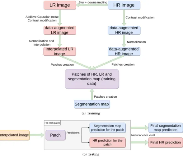
Training. Figure2(a)illustrates the pipeline consid-ered for designing the training, at each epoch. Practi-cally, data augmentation is carried out differently for each epoch and for each image. Indeed, for each im-age and for each epoch, the coefficient used for con-trast modification is randomly drawn, such as the ad-ditive Gaussian noise added to the image.
From these training data, the discriminator and the generator are trained the following way. For each generator weights update, the discriminator weights are updated five times. The training data for the
(a) Generator architecture
(b) Discriminator architecture
Figure 1: Neural network architecture. (a) Generator architecture. (b) Discriminator architecture. See Section3.1.2.
(a) Training
(b) Testing
discriminator are randomly chosen at each iteration, whereas the generator training data successively pass over each batch.
The parameters used for the training are the following: • Adam optimizer parameters similar as in the
original Adam paper [18]; • batch size of 32 patches; • λg p= 100 and λad v= 0.001;
• patch size of 643with a 20 voxels shifting. For each training carried out, the maximal number of epochs is set to 200 and the final weights are those which maximize the performance on a testing data set.
Testing. Figure2(b)illustrates the testing pipeline.
3.2. Implementation and software
The method is implemented in Python 3.6 but the code can also be used in Python 2.7. It was packaged in Pipy2and can be easily installed using the following command:
1 pip i n s t a l l SegSRGAN
However, if GPUs are available, one should install tensorflow-gpu (see installation tutorial3) manually. This implementation is also available on a GitHub repository4which also contains all the weights that we have trained.
The proposed implementation has been developed in order to allow one to train and test arbitrarily any de-rived model from the one initially proposed. This im-plies that the executable Python file (described in Sec-tion3.2.2), and especially the training one, authorizes the tuning of various parameters (see the readme file of the GitHub repository4for more details). Neverthe-less, for the sake of reproducibility, one can find in Ap-pendix Athe parameters that will allow to reproduce the results presented in Section4(training and test-ing).
Hereafter, two main aspects of the implementation will be investigated :
• How one can make quick test of the method. • How one can improve the code.
2https://pypi.org/project/SegSRGAN 3https://www.tensorflow.org/install/gpu 4https://github.com/koopa31/SegSRGAN
3.2.1. The makefile: a solution to quickly run the pro-vided code
One can find in the folder “Test_package_and_local” of the GitHub repository4, a Makefile allowing one to perform quick tests of the method. The Python ver-sion with which one can make the test can be modi-fied in the provided Makefile by changing the value of the $python variable (default value: 3.7).
The only needed external dependency is therefore the Python package “virtualenv” which can be installed using the following command:
1 pip i n s t a l l v i r t u a l e n v
All the implemented commands can be executed in command line, once the working directory of the ter-minal is set to the Test folder:
1 cd / path_to_SegSRGAN_folder / Test_package_and_local Then, one can install the package dependencies, as follows:
1 make create_venv_and_install_SegSRGAN
This command creates a virtual environment and in-stalls all the necessary dependencies. All commands, explained below, use the Python interpreter of this virtual environment (“venv_x” folder where x is the Python version).
Finally, the makefile allows one to test several applica-tions of the provided implementation:
1. testing task (prediction) using the provided trained weights on command line;
2. training task from scratch.
The last requirement before carrying out tests is to add images in the corresponding folders: “Image_for_testing” for testing tasks and “Im-age_for_training” for training ones.
Testing. For testing task, one need to place one or
many images in the “Image_for_testing folder”. Each image need to be placed it in own folder. The com-puted result will be saved in a specific folder, created during the script execution.
Then, one can use the following command to test on the images in the “Image_for_testing” folder as fol-lows:
Training. For training task, the corresponding folder
“Image_for_training” contains two folders named “Label” and “HR”. The training test provided has been designed for training on a sample size of two images (two HR and segmentation maps). The two HR images need to be placed in the “HR” folder whereas the two segmentation maps need to be placed in the “Label” folder.
Then, one can use the following command to test on the images in the “Image_for_testing” folder as fol-lows:
1 make t e s t _ t r a i n i n g
Note that the default parameters for these tests have been chosen in order to ensure acceptable computa-tion times (even with CPUs), but not to obtain the best results.
3.2.2. Scalability and flexibility
In order to make the implementation scalable, the code is organized in multiple files, classes and func-tions. A summary of the code organization is pre-sented below.
In the first level of the package folder (namely “SegSR-GAN/SegSRGAN”) are located the files which can be directly applied to perform a defined task:
• Function_for_application_test_python3.py: pro-vides a Python function for predicting an image; • job_model.py: provides a command line
executable file for predicting multiple im-ages. This file provides an overlay of Func-tion_for_application_test_python3.py;
• SegSRGAN_training.py: provides a command line executable file for training a SegSRGAN model.
In the second level of the package folder (namely “SegSRGAN/SegSRGAN/utils”) are located all the functions used by the three functions presented above.
In the package, one also finds some files / classes which provide a certain scalability to the proposed implementation. The SegSRGAN, ImageReader, nor-malization and interpolation Python files have been designed for such purpose. We now give a short de-scription of these files.
utils/SegSRGAN.py. Used in
“Function_for_applica-tion_test_python3.py” (for testing task) and “SegSR-GAN_training.py” (for training task), this file contains
a class containing all the information about the gen-erator and discriminator architecture.‘ All the func-tions with a name containing “generator_block” or “discriminator_block” correspond to the implementa-tion of the architecture of the generator and the dis-criminator, respectively. Thanks to the use of func-tions, one can easily implement a new architecture (for the discriminator and/or generator) to replace the provided ones.
utils/ImageReader.py. Used in “utils/-patches.py” (for training task) and “Func-tion_for_application_test_python3.py” (for testing task), this file contains all the image readers im-plemented. Each image reader corresponds to a class, whereas an abstract class exemplifies how to implement a new one.
utils/interpolation.py. Used in “utils/-patches.py” (for training task) and “Func-tion_for_application_test_python3.py” (for testing task), this file contains a class which has been de-signed to contain the interpolation methods. Each image interpolation method corresponds to a specific function.
utils/normalization.py. Used in “utils/-patches.py” (for training task) and “Func-tion_for_application_test_python3.py” (for testing task), this file contains a class which has been de-signed to contain the normalization and inverse normalization methods (to put the result image in the same range as the LR image in test).
4. Results
4.1. Data 4.1.1. Datasets
We work on two MRI datasets, namely dHCP5 [14], and the French Epirmex6dataset whose specificities are detailed in Table1.
In particular, the main differences between Epirmex and dHCP datasets are the following:
• the LR images of dHCP are generated;
• dHCP has real segmentation maps and HR im-ages (both with axial resolution of 0.5 mm) whereas Epirmex has not;
5http://www.developingconnectome.org
6Epirmex is part of the French epidemiologic study Epipage 2 [1], http://epipage2.inserm.fr.
dHCP Epirmex
Number of images 40 1500
Coronal resolution
(= Sagittal resolution) 0.5 mm
heterogeneous, mainly
0.45 mm. Histogram of distribution in Figure3(a)
Axial resolution 0.5 mm
(which implies the term of HR image)
heterogeneous, mainly
3 mm (which implies the term of LR image). Histogram of distribution in Figure3(b)
HR Yes No
LR No, generated downsampling HR
from 0.5 mm to 3 mm of axial resolution Yes
Label
(segmentation ground-truth) Yes No
Acquisition machine 3T Achieva
scanner
Various machines from different French hospitals
TR/TE 1200/156 ms
Various, sometimes very different from dHCP (great
heterogeneity in contrast) see Figure4
Table 1: Comparison of dHCP and Epirmex datasets.
0.4 0.6 0.8 0 200 400 600 800
(a) Coronal and sagittal (isotropic) resolution (mm)
3 4 5 0 200 400 600 (b) Axial resolution (mm)
Figure 3: Histograms of the image resolution for the MR images from Epirmex: (a) coronal and sagittal; (b) axial.
• the TR and TE with which the images have been acquired are fixed on dHCP but strongly vary on Epirmex (which induces the motivation to study the training on augmented data modifying the contrast);
• some Epirmex images are noisy, whereas dHCP are not (which induces the motivation to study
Figure 4: Two examples of MR images (axial slices) from the Epirmex dataset. One can observe the differences in terms of con-trast.
the training on augmented data by adding ran-dom noise).
Therefore, in addition to using dHCP for training the model, using it also for testing is relevant since it al-lows us to quantitatively evaluate the result of the method. However, applying the method on Epirmex also makes sense since the LR images are directly ac-quired. In particular, applying the method on these two datasets can provide us with complementary in-formation.
4.1.2. Preprocessing: LR image generation (dHCP)
The dHCP dataset is composed of HR images equipped with binary segmentation (ground-truth), in particular for the cerebral cortex at the same high resolution. As a consequence, in order to train a super-resolution model, we need to determine cor-responding LR images for these couples HR images / segmentation maps.
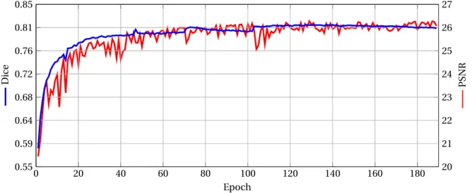
0 20 40 60 80 100 120 140 160 180 20 21 22 23 24 25 26 27 Epoch PSN R 0.55 0.59 0.64 0.68 0.72 0.76 0.81 0.85 D ice
Figure 5: Dice and PSNR evolution during the training on the dHCP dataset.
From a given HR image X , the associated LR image
XLR is generated using the following model, as
pro-posed in [10]:
XLR= H↓B X (12) where B is a blur matrix and H↓ is a downsampling decimation. In particular, we consider a Gaussian fil-ter B with a standard deviation:
σ = res
2p2log2 (13)
where res is the resolution of the LR image.
The generated LR images considered in our experi-mental study are of resolution 0.5×0.5×3 mm3, which is compliant with true clinical data, which are usu-ally strongly anisotropic, as emphasized by the above Epirmex data description.
4.2. Quality metrics
Segmentation. In order to assess the quality of
seg-mentation results, we consider the Dice score [8], which is a standard measure for that purpose. In par-ticular, the adequacy of the computed segmentation S with respect to the ground-truth G is then given as:
Dice(S,G) =2|S ∩G|
|S| + |G| (14)
and lies in [0, 1]. The closer the Dice score to 1, the better the correlation between S and G.
In addition to the quantitative information carried by the Dice score, we also consider the number of con-nected components of the segmented results, noted
NCC. By assuming that the cortex is a connected ob-ject, NCC provides structural information: the higher this value, the lower the topological quality of the ob-ject.
Super-resolution. Measuring the performance of SR
algorithms is less straightforward. Indeed, for gauging the visual aspect similarity between two images, a dis-tance between the intensity of the SR and HR voxels may not be sufficient. The performance of SR recon-struction is then measured by two different indices, namely the PSNR and the SSIM [42], defined respec-tively as: PSNR(X , Y ) = 10log10 ¡ max i Xi ¢2 1 |X | P i |Xi− Yi| 2 (15)
where Xi and Yi are the values of X and Y at point i ,
respectively, and: SSIM(X , Y ) = ¡2µXµY + c1¢ + ¡2σX Y+ c2 ¢ ¡ µ2 X+ µ2Y+ c1 ¢¡ σ2 X+ σ2Y + c2 ¢ (16)
whereµX (resp. µY) is the mean of X (resp. Y )
val-ues,σX(resp.σY) is the standard deviation of X (resp. Y ) values, σX Y is the covariance between X and Y
values, and c1, c2are numerical stabilizers quadrati-cally linked to the dynamics of the image. The SSIM is first computed in each patch of size 7 × 7 × 7 of the assessed image and the final SSIM is then computed as the mean of these patch-wise SSIM measures. For both PSNR and SSIM indices, the higher the value, the better the similarity.
The values of the indices presented hereafter are com-puted only in the intracranial region, defined by the masks provided in the dHCP database.
4.3. Convergence – Training (dHCP)
First, we observe the evolution the Dice and PSNR scores along the training. The values presented here are calculated as follows. The test images are split into patches of size 643voxels, using a 20 voxel shifting (the same used for the training image set). The PSNR and the Dice scores are then calculated in each patch. The final PSNR and the Dice scores are obtained by aver-aging the values computed patch-wise.
The results are depicted in Figure 5, that provides the evolution of the Dice and the PSNR scores at the end of each epoch. The initial Dice has a very low value, close to 0.5, and then increases up to 0.8 rather smoothly. It seems to converge from the 100thepoch. The PSNR also converges, but in a more noisy way. However, the size of the peaks progressively decreases whereas the score tends to stabilize, following the same behaviour as the Dice score.
4.4. Results – Testing (dHCP)
In this section, we present quantitative results related to experiments on the dHCP dataset. In particular, we study the impact of various parameters on the qual-ity metrics used for assessing the relevance of the per-formed SR reconstruction and segmentation. A com-parative study, involving alternative methods can be found in Section5.2.
The results presented here were computed from the 8 images from dHCP used as testing dataset (see Ap-pendix A.4). These results were obtained with patches of size 1283voxels, with a 30-voxel shifting.
4.4.1. Impact of patch overlapping
Impact on the computation time. The time cost of the
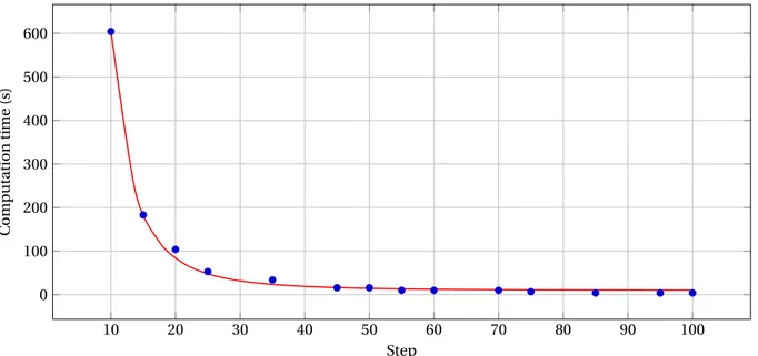
algorithm is directly influenced by the choice of the step (that controls patch overlapping). Indeed, the value of step directly implies the number of patches which have to pass through the neural network. Ac-tually, this number of patches depends directly on the value:
Y
?∈{x,y,z}
n?− pat ch?
st ep (17)
where (nx, ny, nz) is the size of the smallest image
containing the interpolated image and which allows to create an integer number of full patches of size (p at chx, p at chy, p at chz) with st ep between the
suc-cessive patches.
From Equation (17), it is plain that the number of patches is calculated from a quantity that evolves like
st ep−3. Furthermore, even though (n
x, ny, nz) also
depends on the step, one can approximate the com-putation time by an affine function of st ep−3, as con-firmed by Figure6.
The computation times presented in this figure were obtained in the following configuration:
• patch size of 1283;
• on dHCP, which implies that all the HR images which led to the interpolated images are of size (290, 290, 198);
• computation on Tesla P100 GPU and 2 Intel® Xeon™ Gold “Skylake” 6132 CPU.
Here, the computation time varies from 600 seconds (10 min) for a step value of 10, to 4 seconds for a step value of 100, with a st ep−3 decrease between these two values. It is worth mentioning that the de-vice used here processes the patches quickly (approx-imately 5 patches per second) which tends to reduce the impact of the variation of (nx, ny, nz); this could
not be the same on other kinds of devices.
Impact on algorithm performance. We now
investi-gate the impact of the step value on the algorithm per-formance.
For segmentation purpose, the Dice scores obtained on dHCP are provided in Figure 7(a). Here, the patches are still of size 1283voxels. We observe that in any cases, overlapping between patches (i.e. with steps lower than 128) provides better results than without (i.e. with a step of 128). In overlapping cases, the Dice score grows roughly linearly with respect to the size of the step, for reaching values around 0.86 with maximal overlaps, i.e. for steps close to 1. This behaviour for segmentation is confirmed by the behaviour for SR reconstruction, as illustrated by Fig-ures 7(b)–7(c), which provide the PSNR and SSIM scores with respect to the step.
The cortex is a continuous ribbon-like structure. In particular, the connectedness of the segmentation re-sults provided by SegSRGAN is a relevant property, in complement to the three considered quantitative scores. In Figure 8, we show how the value of step between patches influences the number of connected components of the segmented cortex. In theory, only one connected component should be obtained. In other words, obtaining n connected components means that n − 1 parts of the segmented cortex are
10 20 30 40 50 60 70 80 90 100 0 100 200 300 400 500 600 Step C omp u tation time (s)
Figure 6: Computation time (in seconds) against the step value.
erroneously disjoint from the topologically correct structure. Once again, one can observe a linear corre-lation between the error and the value of the step, with close-to-1 values for the higher overlapping / lower steps.
4.4.2. Impact of noise
MR images are generally affected by noise. We now investigate in which extent the performance of the segmentation and SR reconstruction is impacted by adding Gaussian noise to the image. In practice, a Gaussian noise withσ = 2 is added to each voxel of the 8 test MRI images.
The difference between the Dice scores of the seg-mentation results with and without noise, respec-tively, is depicted in Figure9. As expected, the rela-tive Dice scores are slightly better for non-noisy im-ages than for noisy ones, with a gap within [0.03, 0.07]. (Note that from a topological point of view, we also observed that the number of connected components is approximately two times greater in the noisy im-ages compared to non-noisy ones.) We observe that the difference between noisy and non-noisy data in-creases (i.e. the impact of adding noise inin-creases) when the step grows. One can then conclude that the larger the step (i.e. the lower the patch overlapping) the lower the robustness of the method versus noise. In terms of SR reconstruction, we also compared the evolution of SSIM and PSNR with respect to the step value. The results are given in Tables2–3. They
em-Table 2: Mean SSIM scores for SR reconstruction on noisy and non-noisy images (dHCP).
Step Non-noisy Noisy
30 0.73 0.49
80 0.69 0.46
128 0.65 0.44
Table 3: Mean PSNR scores for SR reconstruction on noisy and non-noisy images (dHCP).
Step Non-noisy Noisy
30 26.96 25.40
80 25.85 24.45
128 24.24 23.24
phasize a strong degradation of SSIM, and a much lower degragation of PSNR. As already observed for segmentation results, when increasing patch over-lapping, both scores are significantly improved. For SSIM, the gain between steps sizes of 128 and 30 is of approximately 10% in both noisy and non-noisy cases. For PSNR, it is slightly lower (approximately 8%) with than without noise (approximately 10%).
0 50 100 0.8 0.82 0.84 0.86 Step D ice mean (a) Dice 0 50 100 24 25 26 27 Step PSN R mean (b) PSNR 0 50 100 0.65 0.7 0.75 Step SS IM mean (c) SSIM
Figure 7: (a) Dice scores of segmentation results on dHCP, depend-ing on the step between successive patches of size 1283voxels. PSNR (b) and SSIM (c) scores of SR reconstruction results on dHCP, depending on the step between successive patches of size 1283 vox-els. 0 50 100 0 50 100 Step NC C mean
Figure 8: Number of connected components (NCC) of the seg-mented cortex, depending on the step between successive patches of size 1283voxels; calculated on dHCP database.
0 50 100 0.03 0.04 0.05 0.06 Step D ice diff er en ce bet w e en n o isy and o ri g nal dat a
Figure 9: Difference between the Dice scores with non-noisy and noisy images from dHCP image. Positive values mean that the Dice scores are higher without than with Gaussian noise.
4.4.3. Impact of data augmentation
Motivation. The experiments described until now
have been carried out on dHCP, i.e. an image dataset designed for research purpose, with good properties in terms of noise and signal homogeneity. In real, clin-ical cases, the images forming a dataset are generally of lower quality both in terms of signal-to-noise ratio and signal homogeneity. For instance, all the images in dHCP were acquired with the same TR and TE (im-plying inter-image signal homogeneity); by contrast the TR and TE in Epirmex can strongly vary. Moreover, by contrast with research-oriented datasets, clinical data are generally not equipped with ground-truths; indeed, defining such ground-truths is a complex and time-consuming task that requires heavy work by medical experts. (The same remark also holds for the non-availability of HR images associated to the native
LR ones.) Although our final purpose is to be able to process real, clinical data, it is generally not possible to perform the training on comparable images. Such training then need to rely on dHCP-like data. As a con-sequence, it is indeed relevant to consider data aug-mentation strategies for increasing the ability of the trained networks to take into account real noise and inhomogeneity properties of usual MR images. Fur-thermore, it is known that adding noise to data helps neural networks to increase their generality as inves-tigated e.g. in [15,45].
Data augmentation. The considered data
augmenta-tion on dHCP images consists of applying contrast modification (voxel raised to the power) uniformly drawn in [0.5, 1.5], and adding Gaussian noise with a standard deviation set to 3% of the highest value. Two questions then arise: (1) Does this training im-prove the result on noisy / signal-biased data? (2) Does this training make the performance decrease on the original images? In order to answer these ques-tions, three supplementary families of images, created from the original database, are considered during the testing, namely images:
• with additive Gaussian noise (σ = 2); • with values increased by a square function; • with values decreased by a square root function. Hereafter, these three types of images are denoted as “augmented test dataset”.
Segmentation. The results obtained for segmentation
purpose are depicted in Figure10. First, one can ob-serve that in case of large steps, data augmentation improves more significantly the segmentation results (the best example is when the algorithm is applied without overlapping). However, it is important to keep in mind that the Dice score decreases with respect to the step. In other words, data augmentation al-lows, in a certain extent, to compensate the defects caused by the choice of a large step. In the case of overlapping, the value of step seems to have a neg-ligible quantitative impact on the improvements. In most cases, data augmentation allows to slightly in-crease the robustness of segmentation results, with Dice scores increase between [0.00, 0.03], when con-sidering augmented test datasets. This is not the case for the native dHCP dataset, where the Dice scores are slighly lowered by data augmentation training. In-deed, data augmentation allows the network to learn from a wider range of data; making it more robust with
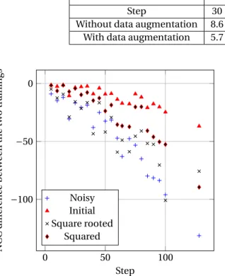
0 50 100 −0.01 0.00 0.01 0.02 0.03 0.04 0.05 Step D ice diff er en ce betw e en th e two tr aining s Noisy Initial Square rooted Squared
Figure 10: Difference between the mean Dice scores of segmenta-tion results when training with and without data augmentasegmenta-tion, de-pending on the step value. Positive (resp. negative) values mean that the Dice scores are better with (resp. without) data augmenta-tion. Computation made on dHCP database.
respect to data variability. As a counterpart, such a versatile network becomes less robust for handling a homogeneous population of data such as dHCP. In complement to the relative evaluation provided by Figure 10, we also propose, in Table 4, an absolute comparison of the Dice scores between segmentation performed with and without data augmentation, both on the dHCP images and their noisy versions. One can observe that the segmentation results for origi-nal dHCP images are slightly degraded (Dice decrease lower than 0.01) with data augmentation, with rea-sons similar to those evoked in the analysis of Fig-ure10. In the meantime, the segmentation results for noisy images are improved (Dice increase from 0.015 to 0.050). In particular, in the case of data augmenta-tion, the difference between Dice scores on standard and noisy images becomes low (approximately 0.015), compared to the case without data augmentation (ap-proximately 0.030 to 0.060). In other words, data aug-mentation makes the segaug-mentation more robust to the tested images, at the price of a loss of specializa-tion with respect to the trained images. However, such trade-off is relevant with respect to real clinical appli-cations.
In order to complete this quantitative segmentation analysis, we also propose, in Figure 11and Table5, a topological analysis of the results, by providing the
Table 4: Mean values of Dice scores for segmentation of dHCP images (noisy and non-noisy) based on standard or data-augmented training.
Original Noisy
Step 30 80 128 30 80 128
Without data augmentation 0.855 0.831 0.805 0.819 0.785 0.740 With data augmentation 0.849 0.827 0.806 0.836 0.812 0.790
Table 5: Mean number of connected components for segmentation of dHCP images (noisy and non-noisy) based on standard or data-augmented training.
Original Noisy
Step 30 80 128 30 80 128
Without data augmentation 8.6 45.3 104.3 26.6 98.5 193.1 With data augmentation 5.7 33.6 61.7 5.8 33.5 61.8
0 50 100 −100 −50 0 Step NC C diff er enc e betw een the tw o tr a in in gs Noisy Initial Square rooted Squared
Figure 11: Difference between the number of connected compo-nents of segmentation results when training with and without data augmentation, depending on the step value. Negative values mean that the number of connected components is lower with data aug-mentation. Calculated on dHCP database.
mean number of connected components of the seg-mented cortex. These topological results strengthen the conclusions obtained for Dice analysis on aug-mented data. In particular, on original data, an improvement is also observed from this topological point of view. Indeed, the number of connected com-ponents is reduced by data augmentation for all types of data studied. In particular, the improvement is im-portant for noisy images. In addition, (see Table5) as for Dice analysis, it appears that segmentation results present very similar topological properties indepen-dently of the noise level of the input images.
SR reconstruction. Concerning SR reconstruction,
Figure12shows the difference of PSNR and SSIM be-tween training with and without data augmentation on original and augmented data. On this figure, it appears that for both SSIM and PSNR, the training with data augmentation (noise and contrast variation) slightly decreases the quality of reconstruction on ini-tial images. This behaviour, already observed in the case of segmentation can be explained by the same factors. However, we also observe that the reconstruc-tion is slightly improved for noisy data, whereas it is slightly degraded for contrast-modified data. These results on noisy images corroborate those of segmen-tation, whereas they are antagonistic in the case of contrast variation. This last point would require to more accurately investigate the specific effects of data augmentation with respect to either noise and con-trast variation.
4.5. Results – Testing (Epirmex)
Result on one example image. In this last part of the
experimental section, we apply our SR reconstruction and segmentation method to the MR images from the Epirmex dataset.
Epirmex contains more than 1 500 images, with very different properties, e.g. the TE and TR values, as dis-cussed above (see Figure 4). These MR images are also of low resolution and a strong anisotropy (see Fig-ure3).
In addition, Epirmex is endowed neither with ground-truth nor with HR images associated to the LR ones, with two main side effects. The first is that the train-ing cannot be carried out on Epirmex images, and it is then mandatory to learn from another dataset, with a data augmentation paradigm; this is what we did with dHCP. Second, there is no objective way of as-sessing the quality of the results, both in terms of
seg-0 50 100 −0.06 −0.04 −0.02 0.00 0.02 Step SS IM diff er en ce betw een th e two tr ai n ing s Noisy Initial Square rooted Squared (a) SSIM 0 50 100 −1.00 −0.80 −0.60 −0.40 −0.20 0.00 0.20 Step PSN R diff er enc e betw een the tw o tr a in in gs Noisy Initial Square rooted Squared (b) PSNR
Figure 12: SSIM (a) and PSNR (b) difference of SR reconstruction between the training with and without data augmentation. Posi-tive (resp. negaPosi-tive) values mean that the metric (PSNR or SSIM) is higher with (resp. without) data augmentation. Calculated on dHCP database
mentation and SR reconstruction. As a consequence, the results provided hereafter have mainly a qualita-tive value.
In particular we propose, in Figure13, some SR re-construction and cortex segmentation results for an MR image representative of the data within Epirmex. Those results were obtained from the parameters learned during the training on dHCP, with data
aug-Step 30 50 80 128
NCC with
data augmentation 30 35 96 387 NCC without
data augmentation 36 53 102 720 Table 6: Mean number of connected components (NCC) computed from 7 Epirmex images.
mentation. A visual analysis of these results leads to satisfactory conclusions. In particular, the segmented cortex is geometrically consistent, with a good visual correlation to the input MR image. Regarding the SR reconstruction, the contrast between the cortex and the surrounding tissues seems higher in the SR image than in the LR one, even in the axial slices, where the resolution is however not modified between LR and SR. Globally, these qualitative experiments on Epirmex tend to corroborate the quantitative ones carried out on dHCP, and to suggest that the proposed method is indeed relevant both for reconstruction and segmentation in the context of real, clinical data anal-ysis.
Due to the lack of ground-truth both for segmention and SR reconstruction, we can rely neither on Dice nor on SSIM and PSNR for assessing the quality of the results on Epirmex. From a topological point of view, it is however possible to assess the structural quality of the segmented cortex, that is assumed to be fully connected.
In particular, the results stated in Table 6 confirm those previously obtained on dHCP (see Table5). Indeed, one can observe that, in case of patch overlap-ping, the number of connected components is better when training with data augmentation. However, the highest difference between these two trainings occurs when the algorithm is used without patch overlapping (i.e. with a step of 128).
Similarly to the experimental results obtrained on dHCP, the evolution of the number of connected com-ponents with respect to the step value argues in favour of reducing as much as possible the step for improving the topological coherence of the segmented cortex. In particular, on Epirmex, the sensitivity of NCC to the number of steps is higher than with dHCP. This can be easily explained by the lower quality of the data, that tends to induce erroneous disconnections, par-tially avoided by increasing patch overlapping.
(a) LR (initial) MR image
(b) SR (reconstructed) MR image
(c) Segmented image (cortex)
Figure 13: (a) LR image from the Epirmex dataset. (b) SR reconstructed image obtained from (a). (c) Segmentation of the cortex obtained from (a) (2D slices and 3D surface rendering).
5. Discussion
5.1. Impact of GAN component ablation (dHCP)
As explained in Section3.1.1, the proposed loss func-tion can be split into two parts. The first is voxel-wise whereas the second derives from the GAN-based ap-proach. In this context, it is then possible to measure in what extent the use of GAN impacts the result. In-deed, by settingλad v to 0, the proposed method is
equivalent to training the generator to perform
super-resolution and segmentation from interpolated image by using voxel-wise loss function, similarly to the be-haviour of a classical neural network-based approach. Furthermore, in addition to making the model more robust to image properties variations, the data aug-mentation strategy also allows the model to output segmentation maps with improved topological prop-erties. For this reason, the following results have been obtained by using data augmentation strat-egy (with the same parameters as in Section 4.4.3):
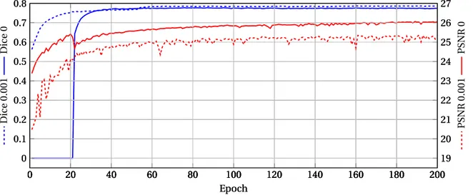
0 20 40 60 80 100 120 140 160 180 200 0 0.1 0.2 0.3 0.4 0.5 0.6 0.7 0.8 0 20 40 60 80 100 120 140 160 180 200 0 0.1 0.2 0.3 0.4 0.5 0.6 0.7 0.8 D ice 0. 001 D ice 0 0 20 40 60 80 100 120 140 160 180 200 19 20 21 22 23 24 25 26 27 Epoch 0 20 40 60 80 100 120 140 160 180 200 19 20 21 22 23 24 25 26 27 Epoch PSN R 0 .00 1 PSN R 0
Figure 14: Dice score (blue) and PSNR (red) evolution during the training on the dHCP dataset. In dashed lines, the results withλad v= 0.001 (initial SegSRGAN value) and in plain line those withλad v= 0 (without the GAN component).
adding Gaussian noise with standard deviation of 3% max value and contrast modification by raising image voxel to a power between [0.5, 1.5].
The results presented in this study investigate the fol-lowing two questions:
1. how the GAN part ablation impacts the training of the method;
2. how it impacts the result obtained in test.
Training. Figure 14 presents the evolution of the PSNR and Dice scores along the training on the aug-mented database. The 8 (one per image) contrast modification coefficients are built such that the points lead to a partition of equal lengths interval of the ini-tial contrast modification interval ([0.5, 1.5]).
In this figure, the two dashed curves show that with the GAN component, the SR and segmentation are learned simultaneously. Indeed, the two curves grow at a comparable rate. By contrast, when the train-ing is done without the GAN component, one can see from tho two solid curves that during the first 20 epochs the Dice score remains null. In the mean-time, the PSNR score rapidly increases. When the 20-th epoch is reached, 20-the Dice score rapidly increases to its convergence point. In the meantime, the PSNR first slightly decreases before increasing slowly until convergence. These experiments suggest that with-out the GAN component, the training is carried with-out in two successive steps: first the model only learns how to perform super-resolution, and then it also learns how to segment. On the contrary, the addition of the
GAN component to the model seems to allow for a si-multaneous learning of both segmentation and super-resolution.
Testing. In this part of the study, all the presented
re-sults are obtained on dHCP images, with a patch size of 1283 and a step of 30-voxel between each patch. In addition, the weights used for the two models are those obtained at the 200th epoch.
Table7presents the results obtained in terms of Dice, NCC, PSNR and SSIM. Globally, these results tend to show that the addition of a GAN component allows to improve the results. However, two quality metrics seem to be more significantly impacted by the addi-tion of the GAN component, namely the PSNR and the NCC.
For the cortex, the Dice is 0.01 higher with GAN com-ponent than without. The mean and the standard de-viation of the NCC is divided by 2 (note, however, that NCC values lower than 10 can already be considered satisfactory).
The two quality metrics show that adding a GAN com-ponent to the model increases the cortical segmenta-tion quality. For the super-resolusegmenta-tion image, the PSNR is slightly higher (+0.35 dB) without GAN component than with. However, it is important to keep in mind that without GAN component, the loss is only based on Charbonnier loss (Eq. (6)) which is close to the MSE, and that by construction the lower the MSE the greater the PSNR. The SSIM with and without GAN component are very close.
Dice NCC PSNR SSIM Without GAN 0.835 ± 0.012 7.75 ± 5.03 27.19 ± 0.76 0.719 ± 0.011
With GAN 0.845 ± 0.015 3.87 ± 2.47 26.84 ± 0.62 0.721 ± 0.012
Table 7: Mean quality metric and standard deviation for SR reconstruction and segmentation with and without GAN component. Calculated over the 8 testing image of dHCP.
PSNR SSIM
SegSRGAN 26.96 0.73
SRReCNN3D 27.79 0.74
Cubic spline interpolation 24.22 0.63 Table 8: PSNR and SSIM mean values. Calculated over 8 dHCP im-ages.
5.2. Comparative study
For the reconstruction part, the proposed method has been compared with cubic spline interpolation and one deep learning-based approach, namely the SR-ReCNN3D method [33]. Concerning the segmenta-tion task, two non-deep learning methods, DrawEM [25] and IMAPA [38], were considered. Two variants of a sequential deep learning-based pipeline have been studied: 1) SR images (obtained from SRReCNN3D) segmented using U-net [36] trained on dHCP data (denoted as SRReCNN3D + U-Net); 2) SR images (obtained from SRReCNN3D) segmented using U-net trained on SRReCNN3D reconstructed data (denoted as SRReCNN3D + U-Net?). The U-Net architecture has 2 levels of downsampling for the encoder and 28 feature maps for the first convolution (value chosen such as U-Net has comparable numbers of weights as SegSRGAN generator) and the used loss is the binary cross entropy. This implementation is also available on a github repository7. As in typical clinical settings, these methods have been applied on interpolated im-ages (using cubic spline interpolation).
The results presented here were computed from the 8 images from dHCP used as testing dataset (see
Appendix A.4). These results were obtained with patches of size 1283voxels, with a 30-voxel shifting. All the comparison results have been obtained using the same training and testing base from dHCP. Table 8 summarizes reconstruction performances through PSNR and SSIM. One can observe that the two quality scores for the SR image reconstruction exhibit better results with SegSRGAN than with cu-bic spline interpolation (which constitutes a standard baseline and is the input of the network). As expected,
7https://github.com/koopa31/SegSRGAN
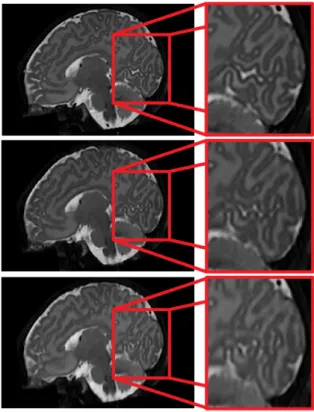
Figure 15: Reconstruction results (sagittal view). Top: HR image (dHCP database). Middle: SegSRGAN SR image. Bottom: SR-ReCNN3D SR image.
the PSNR is higher with SRReCNN3D than with SegSRGAN (+0.8 dB). This is because SRReCNN3D uses MSE as loss function, contrary to SegSRGAN. However, the SSIM scores are comparable between SegSRGAN and SRReCNN3D. From a more qualitative / visual point of view, when carefully observing SR im-ages obtained with SegSRGAN and SRReCNN3D (see e.g. Figure15), the fine details, especially in the cortex (sharpness, contrast and continuity) in the real image are closer to those observed in the SR image obtained with SegSRGAN than with SRReCNN3D.
Table 9 summarizes the Dice scores. It can be seen that, quantitatively, the deep learning-based approaches lead to better cortical segmentation re-sults with significant improvement with respect to DrawEM and IMAPA. It has to be noticed that, as
Dice DrawEM 0.730 ± 0.010 IMAPA 0.786 ± 0.023 SRReCNN3D + U-Net 0.829 ± 0.019 SRReCNN3D + U-Net? 0.861 ± 0.011 SegSRGAN 0.855 ± 0.014
Table 9: Dice mean values and standard deviations for segmenta-tion maps. Calculated over 8 dHCP images.
NCC SRReCNN3D + U-Net 9.25 ± 3.86 SRReCNN3D + U-Net? 4.00 ± 2.39
SegSRGAN 8.62 ± 3.27
Table 10: NCC mean values and standard deviations for segmenta-tion maps. Calculated over 8 dHCP images.
mentioned in [38], the application of IMAPA on orig-inal HR dHCP images leads to a mean Dice score of 0.887 ± 0.011. In other words, the result obtained with SegSRGAN on interpolated images, only decreases by 0.03 compared to IMAPA applied on HR images. Regarding the deep learning-based techniques, it can be seen that learning two networks independently (SRReCNN3D + U-Net method) leads to sub-optimal results. The other way around, the use of SRReCNN3D + U-Net?and SegSRGAN leads to similar Dice scores. However, one may keep in mind that the proposed SegSRGAN method performs joint learning, whereas the method SRReCNN3D + U-Net?uses a sequential approach, which implies a complexity of implemen-tation and a longer learning time.
To complete the segmentation evaluation, Table 10
provides NCC values for deep learning-based tech-niques, showing the three methods lead to satisfac-tory results. Figure16provides complementary vi-sual segmentation quality analysis, showing the high quality of the segmentation results. Finally, similarly to the SR comparative study, this quantitative analysis would require to be completed by a thorough qualita-tive analysis, also based on topological and geometri-cal metrics; however, this falls out of the scope of this article.
5.3. Limits of the method
The application of the method on the Epirmex database revealed some limits of our approach af-ter training on dHCP. Actually, the main limit derives from the difference between the Epirmex images and the dHCP ones. Even if the data augmentation strat-egy tends to reduce these differences, it is not possible
(a) Ground-truth
(b) SegSRGAN
(c) SRReCNN3D + U-net?
(d) SRReCNN3D + U-net
Figure 16: 3D view of (a) Ground-truth, and segmentation results from (b) SegSRGAN, (c) SRReCNN3D + U-net?, (d) SRReCNN3D + U-net.
to fully take into account all the existing differences, by considering only simple image transformations.
Figure 17: Slice of an Epirmex image leading to segmented tissues outside the intracranial region.
Figure 18: Slice of an Epirmex image altered by bias effect, leading to segmentation errors.
In particular, this is illustrated in Figure17where we can see some extracranial tissues which are not (or al-most not) visible in dHCP images. A simple heuris-tics for tackling this issue could consist of coupling the proposed pipeline with a standard skull stripping pre-or post-processing.
Another type of limit of the proposed method con-cerns the quality of the images. Indeed, some artifacts such as movement between successive slices, slices with lower contrast compared to the overall volume, or intensity bias within a given slice, tend to deterio-rate the obtained segmentation. An example of slice altered by bias effect is exemplified in Figure18. One can see that in the area of lower intensity, the method fails to correctly segment the cortex. Furthermore, be-cause of the receptive field (the region of the input space affects a particular layer) of the generator, an ar-tifact on one area of the image may alter a wider area on the result image.
6. Conclusion
In this article, we have proposed a new methodolog-ical and software solution for performing SR recon-struction and segmentation from complex 3D MR im-ages. Our framework, based on generative adversar-ial networks has been described in detail, both from theoretical and technical points of view. In particular, a free, documented software version is available, for
dissemination to the scientific and clinical communi-ties and for the sake of reproducibility of the results. Although our purpose was not to carry out a compar-ative work with other methods (we do not claim the superiority of our method, but its usefulness in cer-tain contexts), we have proposed a consequent exper-imental analysis in the case of cortex investigation in the neonate. This experimental analysis, carried out on both research and clinical datasets, and from qual-itative and quantqual-itative points of view, tend to prove the relevance of our approach, with satisfactory re-sults both in terms of SR reconstruction and segmen-tation.
In particular, the ability of the method to take ad-vantage of data-augmentation strategies allows one to involve it for SR reconstruction and segmenta-tion of clinical datasets, which are generally not en-dowed with ground-truth and/or examples of high-resolution MR images associated to LR ones. In this context, it was observed that carrying out a learning procedure on a research dataset, whereas degrading the data (e.g. in terms of noise and intensity bias) con-stitutes a tractable approach.
Of course, the proposed method is not specific to the cortex, and it could also be used for other kinds of cerebral structures in MRI. The segmentation re-sults obtained on the cortex are indeed satisfactory. However, since the segmentation and SR reconstruc-tion are handled in a common way, it is possible that the quality of SR reconstruction may be impacted by the structure of interest targeted for segmentation. In other words, it is possible that the SR reconstruc-tion may be more efficient in the neighbourhood of the cortical ribbon, compared to other loci in the brain. A way of tackling this issue would be to con-sider a more global segmentation purpose, involv-ing the main cerebral tissues in parallel, leadinvolv-ing to a more global guidance of SR reconstruction by the information carried by segmentation. In theory, this is indeed possible, since the method architecture can allow multi-segmentation, whereas research datasets are indeed equipped with complete ground-truth de-fined as atlases.
Regarding perspective works, from a methodological point of view, we will more deeply investigate the trade-off between computational cost and result qual-ity, in particular with respect to data variability within MR image cohorts. We will also study the effects of adding noise to the label / segmentation maps of the training data in order to assess the potential side ef-fects with respect to the generalization of the method. More generally, we will experimentally assess the
vari-ous consequences on data augmentation with respect to usual features likely to degrade MR image quality, namely noise, signal bias, contrast heterogeneity, or movement artifacts. From a more applicative point of view, our next purpose will consist of processing large image cohorts for automatically extracting regions of interest, in a clinical context.
Acknowledgements
The research leading to these results has been supported by the ANR MAIA project, grant ANR-15-CE23-0009 of the French National Research Agency
(http://recherche.imt-atlantique.fr/maia);
INSERM and Institut Mines Télécom Atlantique (Chaire “Imagerie médicale en thérapie
intervention-nelle”); the Fondation pour la Recherche Médicale
(grant DIC20161236453); and the American Memorial Hospital Foundation. We also gratefully acknowledge the support of NVIDIA Corporation with the donation of the Titan Xp GPU used for this research.
References
[1] P.-Y. Ancel, F. Goffinet, and EPIPAGE 2 Writing Group. EPIPAGE 2: A preterm birth cohort in France in 2011. BMC Pediatrics, 14:97, 2014.
[2] G. Ball, J. P. Boardman, P. Aljabar, A. Pandit, T. Arichi, N. Mer-chant, D. Rueckert, A. D. Edwards, and S. J. Counsell. The influence of preterm birth on the developing thalamocortical connectome. Cortex, 49(6):1711–1721, 2013.
[3] G. Ball, L. Srinivasan, P. Aljabar, S. J. Counsell, G. Durighel, J. V. Hajnal, M. A. Rutherford, and A. D. Edwards. Development of cortical microstructure in the preterm human brain.
Proceed-ings of the National Academy of Sciences of the United States of America, 110(23):9541–9546, 2013.
[4] M. J. Cardoso, A. Melbourne, G. S. Kendall, M. Modat, N. J. Robertson, N. Marlow, and S. Ourselin. AdaPT: An adaptive preterm segmentation algorithm for neonatal brain MRI.
Neu-roImage, 65:97–108, 2013.
[5] P. Charbonnier, L. Blanc-Féraud, G. Aubert, and M. Barlaud. Deterministic edge-preserving regularization in computed imaging. IEEE Transactions on Image Processing, 6(2):298–311, 1997.
[6] Y. Chen, Y. Xie, Z. Zhou, F. Shi, A. G. Christodoulou, and D. Li. Brain MRI super resolution using 3D deep densely connected neural networks. In ISBI, Proceedings, pages 739–742, 2018. [7] P. Coupé, J. V. Manjón, V. Fonov, J. Pruessner, M. Robles, and
D. L. Collins. Patch-based segmentation using expert pri-ors: Application to hippocampus and ventricle segmentation.
NeuroImage, 54:940–954, 2011.
[8] L.R. Dice. Measures of the amount of ecologic association be-tween species. Ecology, 26:297–302, 1945.
[9] J. Dubois, M. Benders, A. Cachia, F. Lazeyras, R. Ha-Vinh Leuchter, S. V. Sizonenko, C. Borradori-Tolsa, J. F. Man-gin, and P. S. Hüppi. Mapping the early cortical folding process in the preterm newborn brain. Cerebral Cortex, 18(6):1444– 1454, 2008.
[10] H. Greenspan. Super-resolution in medical imaging. The Computer Journal, 52(1):43–63, 2008.
[11] L. Gui, R. Lisowski, T. Faundez, P. Hüppi, F. Lazeyras, and M. Kocher. Morphology-based segmentation of newborn brain MR images. In MICCAI NeoBrainS12, Proceedings, pages 1–8, 2012.
[12] I. Gulrajani, F. Ahmed, M. Arjovsky, V. Dumoulin, and A. C. Courville. Improved training of Wasserstein GANs. In NIPS,
Proceedings, pages 5769–5779, 2017.
[13] M. Hack and A. A. Fanaroff. Outcomes of children of extremely low birthweight and gestational age in the 1990s. Seminars in
Neonatology, 5:89–106, 2000.
[14] E. Hughes, L. Cordero-Grande, M. Murgasova, J. Hutter, A. Price, A. Santos Gomes, J. Allsop, J. Steinweg, N. Tu-sor, J. Wurie, J. Bueno-Conde, J.-D. Tournier, M. Abaei, S. Counsell, M. Rutherford, M. Pietsch, D. Edwards, J. Haj-nal, S. Fitzgibbon, E. Duff, M. Bastiani, J. Andersson, S. Jbabdi, S. Sotiropoulos, M. Jenkinson, S. Smith, S. Harrison, L. Grif-fanti, R. Wright, J. Bozek, C. Beckmann, A. Makropoulos, E. Robinson, A. Schuh, J. Passerat Palmbach, G. Lenz, F. Mor-tari, T. Tenev, and D. Rueckert. The Developing Human Con-nectome: Announcing the first release of open access neona-tal brain imaging. In OHBM, Proceedings, 2017.
[15] I. Isaev and S. Dolenko. Adding noise during training as a method to increase resilience of neural network solution of in-verse problems: Test on the data of magnetotelluric sounding problem. In NEUROINFORMATICS, Proceedings, pages 9–16, 2017.
[16] J. Johnson, A. Alahi, and L. Fei-Fei. Perceptual losses for real-time style transfer and super-resolution. In ECCV, Proceedings, pages 694–711, 2016.
[17] H. Kim, C. Lepage, A. C. Evans, J. Barkovich, and D. Xu. NEO-CIVET: Extraction of cortical surface and analysis of neonatal gyrification using a modified CIVET pipeline. In MICCAI,
Pro-ceedings, pages 571–579, 2015.
[18] D. P. Kingma and J. Ba. Adam: A method for stochastic opti-mization. CoRR, abs/1412.6980, 2014.
[19] W.-S. Lai, J.-B. Huang, N. Ahuja, and M.-H. Yang. Deep Lapla-cian pyramid networks for fast and accurate super-resolution. In CVPR, proceedings, pages 624–632, 2017.
[20] C. Ledig, L. Theis, F. Huszár, J. Caballero, A. Cunningham, A. Acosta, A. Aitken, A. Tejani, J. Totz, Z. Wang, and W. Shi. Photo-realistic single image super-resolution using a genera-tive adversarial network. In CVPR, Proceedings, pages 105–114, 2017.
[21] J. Lefèvre, D. Germanaud, J. Dubois, F. Rousseau, I. de Macedo Santos, H. Angleys, J.-F. Mangin, P. S. Hüppi, N. Girard, and F. De Guio. Are developmental trajectories of cortical folding comparable between cross-sectional datasets of fetuses and preterm newborns? Cerebral Cortex, 26(7):3023–3035, 2016.
[22] P. Luc, C. Couprie, S. Chintala, and J. Verbeek. Semantic seg-mentation using adversarial networks. CoRR, abs/1611.08408, 2016.
[23] D. Mahapatra. Skull stripping of neonatal brain MRI: Using prior shape information with graph cuts. Journal of Digital
Imaging, 25:802–814, 2012.
[24] A. Makropoulos, S. J. Counsell, and D. Rueckert. A review on automatic fetal and neonatal brain MRI segmentation.
Neu-roImage, 170:231–248, 2017.
[25] A. Makropoulos, I. S. Gousias, C. Ledig, P. Aljabar, A. Serag, J. V. Hajnal, A. D. Edwards, S. J. Counsell, and D. Rueck-ert. Automatic whole brain MRI segmentation of the devel-oping neonatal brain. IEEE Transactions on Medical Imaging, 33(9):1818–1831, 2014.