HAL Id: hal-00696970
https://hal-mines-paristech.archives-ouvertes.fr/hal-00696970
Submitted on 14 May 2012HAL is a multi-disciplinary open access
archive for the deposit and dissemination of sci-entific research documents, whether they are pub-lished or not. The documents may come from teaching and research institutions in France or abroad, or from public or private research centers.
L’archive ouverte pluridisciplinaire HAL, est destinée au dépôt et à la diffusion de documents scientifiques de niveau recherche, publiés ou non, émanant des établissements d’enseignement et de recherche français ou étrangers, des laboratoires publics ou privés.
Modeling Novelty-Driven Industrial Dynamics with
Design Functions: understanding the role of learning
from the unknown
Pascal Le Masson, Armand Hatchuel, Benoit Weil
To cite this version:
Pascal Le Masson, Armand Hatchuel, Benoit Weil. Modeling Novelty-Driven Industrial Dynamics with Design Functions: understanding the role of learning from the unknown. International Schumpeter Society Conference, 2010, Denmark. pp.28. �hal-00696970�
page 1 / 28
MODELING NOVELTY
-
DRIVEN INDUSTRIAL DYNAMICS WITHDESIGN FUNCTIONS
:
UNDERSTANDING THE ROLE OF LEARNINGFROM THE UNKNOWN
Pascal Le Masson*, Armand Hatchuel, Benoit Weil
*corresponding author :
Ecole des Mines de Paris, 60 Bvd Saint Michel, 75 272 Paris Cedex 06 Tel : +33 1 40 51 92 21 ; Fax : +33 1 40 51 90 65
[email protected], [email protected], [email protected] Keywords : knowledge dynamics, design function, design regime, industrial dynamics, innovation ISS research area:
• Technological change and industrial evolution in economic development
Aknowledgements: This work was supported by the ANR program “Entreprise”, project RITE (ANR-07-ENTR-011-RITE) and the chair “design theory and methods for innovation”
Abstract
In his synthesis on industrial dynamics, Malerba called for a renewal of the models for the dynamic analysis of innovation and the evolution of industries [1]. To go this way we investigate the relationship between knowledge dynamics, innovation dynamics, and sectoral growth in the particular case of Schumpeterian “development” [2]. Our analysis is based on a model where economic actors (suppliers and customers) are represented by design functions, endogenizing the generation of “unknown” products, the regeneration of competences and of utility functions. We use the model to simulate four situations of industrial dynamic characterized by the (successful or impeded) emergence of novelty: automotive industry, pharmaceutical and biotech industry, semiconductor industry and orphan innovation in cleantech. This model shows that the success of “novelty-oriented” industrial dynamics depends on the efficiency of the coupling between design functions in the economy. We show that 1) good suppliers’ profit and customers user-value relies on a sparing of knowledge
and novelty; 2) coupling is based less on the initial level of competences and knowledge
capitalization than on learning from “unknown” products; 3) learning from the unknown creates externalities, so that the exploration of the unknown appears as a new kind of “common good”.
page 2 / 28
Introduction: the aim of the study: modeling industrial dynamics in
novelty creation situations, based on design functions.
In several industrial sectors appear today surprising industrial dynamics: semiconductor industry is characterized by a fascinating pace of science-based innovation, fascinating because the pace is very fast but also because this high pace is extremely stable over decades; car industry, considered as the stable reference for the dominant design model since the works of Abernathy and Utterback is today confronted to an increasing request of innovation coming from consumers; in cleantech, and particularly in fuel cells, one can be struck by the paradoxical situation of high investments in technology development, high social expectations and surprisingly low results in term of economic growth: this reveals a paradoxical situation of orphan innovation where social demand ishigh, technology developments are intensive but the growth remains low.
These phenomena are now well-known in the literature. However we find only partial and ad’hoc explanations of these new industrial dynamics. Yet these situations are actually belonging to the same class of industrial dynamics, namely the calss of Schumpeterian “development” [2,3 ,4], ie situations where the parameters of the Walrasian system are changed « in such a way that this transition cannot be decomposed into infinitesimal steps » [2]. In his recent synthesis on industrial dynamics and sectoral evolutions, Malerba appealed to “move from the statement that everything is changing with everything else” [1] and called for a renewal of the models for the dynamic analysis of innovation and the evolution of industries. To go this way we propose in this paper a new framework to analyse these industrial dynamics: we show that we can interprete these dynamic in a theoretical framework based on design activities. We use an economy model of “design functions” [5] to investigate the relationship between knowledge dynamics, innovation dynamics, and sectoral growth in the particular case of Schumpeterian “development” [2, 3 ,4].
In a first part we make a brief overview of the literature on industrial dynamics in case of Schumpeterian development. We are led to identify three main gaps in the literature: 1) we lack models of learning processes in “novelty” situations; 2) in particular such a model should better address the relationship between knowledge production, innovation and growth; 3) such a model should lead to discuss institutional logics supporting “novelty”. In a second part we present the model of an economy built on a representation of economic agents as designers and introduce the simulation. In a third part we present the results of the simulation. In the last part we discuss the main conclusions.
I. Literature review: industrial dynamics to the test of
Schumpeterian development.
Schumpeterian “development” (also called “novelty”) opens two critical issues for the literature on industrial dynamics. Classical models of industrial dynamics are based on two assumptions: knowledge implies innovation and innovation implies growth. In case of “novelty”, both assumptions are questionable:
1- Knowledge dynamics and innovation dynamics should be distinguished: the hypothesis of growth determined by the level of of codified knowledge has been thoroughly criticized in the literature [6] ; analysis of the R&D paradoxes have already underlined that there is no clear correlation between R&D intensity and the growth of
page 3 / 28
the firm [7-11]; as shown in studies of radical innovation processes [12] and science-based innovation [13], “novelty” is more than “applied research”: it comes from processes of experiential learning [14] or learning cycles [15], where competences stem from the sequence of innovative projects. Formally speaking novelty raises critical issues to the basic model of “knowledge for innovation”, namely the model of absorptive capacity [16,17]: as explained by Cohen and Levinthal absorptive capacity represents the capacity of a company to use external knowledge for developing innovative products; this capacity can be assimilated to the internal level of R&D as long as internal R&D has a capacity to recognize the value of external knowledge [18]. But radical innovation precisely aims at revising the value criteria hence severely weakening existing absorptive capacity [18 ,19,20 ,21]. We need a model based on a richer link between knowledge and innovation: instead of a “production” model, where knowledge appears as a production factor and innovation as an output we need to model how knowledge and passed innovation lead to new innovation and new knowledge. This is one basic feature of a “design function”.
2- Innovation dynamics and growth are not necessary linked: creative destruction can lead to destroy demand side competences and hence utility functions of the consumers, resulting in negative economic growth. As mentioned by Witt, “why consumer behavior changes during the process of economic growth” is hardly discussed in the literature (p. 24) [22]. Models have been proposed, considering customer with its own absorptive capacity [23]. As a matter of fact, such models have the same limits as absorptive capacity itself, since they consider that customer’s absorptive capacity increases with the proximity between the new products and the products that customer already know, which can explain slowdown in the diffusion of radical innovation but hardly explain the mere existence of radical innovation. For modeling changes in customer behaviors some guiding principles have been provided by Georgescu-Roegen [24], mentioning a principle of non-satiety (old goods and services are likely to occupy a decreasing share of individual and household budgets, thus making room for the adoption of new ones) and a principle of the growth of wants. Rosenberg has described processes of learning by using [25], suggesting similar processes as the one seen from the innovator point of view in innovation processes: knowledge does not precede the process but can be acquired during the innovation process, by confrontation with innovative products. Here also we need to enrich the model of customer knowledge and utility revision. Customer appears as a kind of “design function”.
Hence novelty situations invite to revise the classical assumptions of a deterministic relationship between knowledge dynamics, innovation dynamics and economic growth and raise to issue: how to endogeneize learning from the product design experiments? How to endogeneize the evolutions of the customer utility function?
Several models of industry dynamics have already been proposed. It is impossible to review all of them in this paper; one can underline some dominant features in these models:
1- A first class of models are the models of endogenous growth. An archetypal example being Aghion and Howitt model (and the most recent variants) [26-28] called Schumpeterian Growth model. It is interesting to note that such models do not address novelty issue (since the list of future goods is known ex ante and customers preferences are not considered in the model) nor learning issues: learning is still exogenous [5] in the sense that R&D investment determine innovative product (deterministic link from knowledge to innovation) and innovation has no effect on
page 4 / 28
knowledge itself (no endogenous learning from innovative products). The relationship between competence and growth in these models has been strongly criticized [29,30]. 2- A second class of models are the models of product life cycle, mainly models of the
emergence of an industry dominant design. These models tend to explain the transition from an emerging industrial sector to its stabilization, this transition being characterized by well-identified patterns (product innovation, process innovation, entry and exit, number of firms on the market, levels of R&D investments,…) [31 ,32,33]. Beyond the seminal Works of Abernathy and Utterback, who focused on the relationship between the level of R&D investment and the level of uncertainty (« as the enterprise develops, uncertainty about markets and appropriate targets is reduced, and larger R&D investments are justified »), two main models have been developed: a first one is the « supply-side » approach based on return appropriation [33] – this model explains the competition structure but doesn’t consider growth nor learning (see lemma 2, p. 569 : the quantity of product produced by a firm is constant over time depends only on the time of entry and the initial level of expertise) ; a second one is the demand-side approach [34 ,35,36]. In the second approach, models not only explain dominant design but also constant increase of performance level on a known function and the demand conditions that enable disruptive innovation. However these models don’t address the novelty issue as far as they don’t consider the « discovery » and learning of new utility by the customers (disruptive innovation is actually modeled as a supply side adaptation to a pre-existing demand-side functional variety).
This brief overview shows that existing models only partially address the issue of novelty, growth and learning. Moreover literature has already mentioned several exceptions to the dominant design patterns: Klepper mentions: i) petrochemicals, disposable diappers, zipper,… (in the time period 1930-1970) where process specialists appear, ii) medical diagnosis imaging products, ATM,… where incumbent captures product innovation or forms of symbiosis unfold (in the 1980s), iii) submarket specialization as in business jet and lasers (characterized by taste differentiation). Recent research on industrial dynamics have analysed new phenomena: they describe new forms of competitions through innovation (the creation of market disequilibria, see [37]), new industry life cycle (far from classical Abernathy and Utterback dominant design establishment, see [32,38]) and new sectoral evolutions based on new coupled dynamics of demand and technology [22,23], and the increasing involvement of economics actors like users [39], industrial partnerships [40] or platform leaders [41]. These new features of industrial dynamics are usually analysed in terms of knowledge dynamics and absorptive capacity (see for instance [38,42],…) but we miss an integrated framework to analyze those kind of situations.
This review helps to identify clear gaps in the literature:
1. There is a lack of a theoretical and accurate model of learning processes and utility evolutions in situations of “novelty”, where radical innovations lead to change the whole Walrasian vector of the economy.
2. Such a model would help to figure out several forms of relationships between i- knowledge dynamics for firms and consumers, ii) innovation and iii) economic growth.
3. Such a model should suggest new approaches of the relationship between actors, accounting for networks, externalities and common goods in novelty-oriented economies.
page 5 / 28
II. Method: model and simulation of an economy based on design
agents.
II.A. A model of design functions
Following Schumpeter’ definition of innovation [43]: "we will simply define
innovation as the setting up of a new production function", a model of the innovative firm
must go beyond established production functions and requires the modelling of this “setting
up” function.
We introduce a new function for innovation that we have called the "design function" inherent to firms. In formal terms, we define a design function over two spaces: the space of goods (including capital) G and the space of knowledge K; the design function is a function of both spaces over each other.It transforms the space of goods and the space of knowledge by “expansion” [44]. Design F: G x K! expand(G x K). (where expand(GxK) is the expanded G and K spaces) [5]. An innovation appears as a regeneration of the space of goods (G). Innovation is not necessary linked to a technical advance in K space.
Let us compare a "design function" defined in this way and the traditional micro-economic production function. The production function models the way in which the combination of
quantities of production factors, usually capital (including intermediary goods) and labour (or
competencies), serve to make a quantity of one or several goods. The nature of these goods is implicit to the production function itself and, in principle, the list of goods given ex ante is not modified by the production activity. In formal terms, a production function is traditionally written as: Production F: G x K ! Q(G): Q(G) being a function quantified over the
space of goods (the space G and the space K are not transformed).
In contrast, the design function has the following characteristics:
• The inputs of a design function are goods (including capital) and competencies, • The outputs of a design function are:
" A definition of the goods to be produced (which can also be a revision of existing goods or can involve the withdrawal of these goods).
" A definition of the processes required to produce and distribute these goods (production function of the goods; once again, this may be a variation on existing processes, or may involve the withdrawal of the processes).
" For each type of competency, the learning which results from the design work and feedback on experience from the product (in manufacturing, in the market, etc.). This list matches the frequent empirical observation whereby a company can sell either products (goods or services) or production functions (design of turnkey factories), or design competencies that can be as abstract as a patent, a name, a drawing or a brand. • The production function is a restriction of the design function: It can be noted that a
traditional production function is a restricted design function whose final space is restricted to quantities of goods, and which does not "reproduce" any of the input factors! Yet the distinctive feature of design processes is that they reproduce or deform an initial competency and/or initial goods. In formal terms, we move from the production function to the design function by symmetrizing the initial and final spaces.
• Recursiveness of design functions: This formal symmetry enables us to consider the repetition of design activities as a recursive function within a given firm, i.e. as something that transforms itself by its own action. In order to model the history of the firm, we can thus start with a design function and see how it is repeated over time. Formally, let there be a design function relating to a firm's design project and let the initial inputs be vectors
page 6 / 28
Ginputs and Kinputs, f (Ginput, Kinput). The general function of the firm after k design projects
can be set down as: ffirme = f o f o…o f(Ginput, Kinput) = fn (Ginput, Kinput).
The design function enables us to model a richer relationship between knowledge dynamics and innovation: new products are accompanied by knowledge created (and not preceded by it) and knowledge created at time t can be reused at time t+1.
The model of the design function can be generalized for the customer. As suggested by Witt [22]: “people reflect and learn about how to instrumentalize direct inputs and the services of tools for the satisfaction of their wants”. According to this model, a consumer (or generally speaking: a buyer) uses the goods is has bought to design actions (usages; but if the buyer is a company, this could also be goods) according to his wants, based on his own competences. From the buyer point of view, he designs usages (or new goods) based on his own competences (including the acquired goods) and the list of existing usages. The buyer can hence be modeled as a design function that take in input competences (competence in usages design and acquired goods, considered as tools for designing new usages) and existing usages) and giving in output new competences (better capacity to use the tools, better understanding of the value of some usages,…) and new usages. The buyer expands his space Usages x Competences just like the firm expands its space Goods x Competences. This model is self evident if the buyer is a design company.
In formal terms:
(Consumer) Design F: U x K! expand(U x K), where K=(Kbuyer, Gbought)
In this model, user value appears as a competence of the user to appreciate a new usage. It can be transformed over time through the design function. Hence the model is adapted to model a richer relationship between product innovation and transformations of the user value. Moreover a new product proposed by a company can lead to design a new usage.
II.B. Simulating novelty-oriented industrial dynamics
Based on this model, our issue is to analyze novelty-oriented industrial dynamics. Our method is twofold:
1- we simplify the general model into a simulation model that will enable us to simulate specific situations.
2- we identify four archetypal situations of “novelty-oriented” industrial dynamics and try to analyse these situations with the help of the simulation process.
We detail now these two steps.
II.B.1- U-K simulation model
We simplify supplier design function:
• At each design step the list of goods can be changed in two ways: either by the improvement of existing products in known direction (the car consumes a bit less fuel), this creates an extension of the list of products in a known direction, we call this type of innovation a K-type innovation (K for known); or by the creation of a product which is fully unknown, called a U-type innovation (a car for car sharing). Each product is characterized by its cost.
page 7 / 28 ! cK, S i(t) = cK0. KS 0 KS i(t)
where cK0 and KS0 are constants and KSi(t) is the competence
level of the firm Si at time t. The form of the curve is guided by a classical
“diminishing return” hypothesis. U-type innovation has a unit cost:
!
cU = cU0 where cU0 is constant. In this version of
our model there is no difference in firms capacities to design U-products. • The firm profit is:
!
"Si(t) = ( pK # cK , Si(t)). QK , Si + ( pU # cU). QU , Si
• At each design step, knowledge evolves depending on the product that has been designed during the step. The equation is:
!
KSi, t +1=
KSi, t
(1+ iS" iSi)
+#Si. QU , Si(t) where KSi, t is the competence level of the firm Si at
time t. iS is an actualization parameter, representing the way knowledge becomes
obsolete in a particular sector (on the supply-side of this sector), iSi is the capacity of
the firm Si to learn from using its KSi base (“learning by doing”) ie to increase its
competence level by using it, !Si is the capacity of the firm Si to learn from the
unknown, QU,Si(t) is the quantity of unknown products sold by the firm S during the
time period from t to t+1.
To give a simple example: if iS=0%, iSi=5% and QU(t) =0, the firm didn’t sold
U-product during the time period t to t+1. Thanks to iSi=5%, the knowledge base has
increased from K to 1,053.K. In a “turbulent” sector one could have i=55%. In this case the knowledge based goes from K to 0,66.K: this means that at time t+1 the firm competence level has “decreased” because of the speed of competence obsoleteness in the sector. For instance in semiconductor industry, where each product generation is a scientific and technological challenge, the competence level reached at a technology generation t represents only a relatively low level for the technology generation t+1. We also simplify buyer design function, in a similar way:
• If the buyer has bought a K-type product, then it will design a usage that is an improvement of an usage that was already known from past experience. If the buyer buys a U-type product, he will invent an unknown usage. The known usage brings a unitary user value:
!
µK , Bj(t) =µK0.
KBj(t)
KB 0
where !K0 and KB0 are constants and KBi(t) is the competence
level of the buyer Bj at time t. The form of the curve is guided by a classical
“diminishing return” hypothesis.
U-type usages have a unitary user value:
!
µU =µU0 where !U0 is constant.
• The buyer user value is:
! UVBj(t) =µK , j(t).QK,Bj " (t) # pK(t) QK , Bj(t) +µU.QU ,Bj " (t) # pU. QU , Bj(t)
• At each design step, knowledge evolves depending on the user value that has been designed during the step. The equation is:
page 8 / 28 ! KB j, t +1= KB j, t
(1+ iB " iBj)+#Bj. QU , Bj(t) where KBj, t is the competence level of the buyer
Bj at time t. iB is an actualization parameter, representing the way knowledge becomes
obsolete in a particular sector on the demand-side, iBj is the capacity of the buyer Bj to
learn from using its K base (“learning by using”) ie to increase its competence level by using it, !Bj is the capacity of the buyer Bj to learn from the unknown, QU,Bj(t) is the
quantity of unknown products bought by the buyer Bj during the time period from t to
t+1.
A sector is characterized by iS, iB, cU, !U. A sector has two sellers (no entry after t=0)
(i"{1, 2}). The sellers Si can have different characteristics (differences in KSi(t=0), in iSi, in
!Si). One sector has a defined number of buyer nB (taken conventionally equal to 10 in the
simulation). To simplify all buyers have the same iBj and yBj, #j There are differentiated by
their initial competence level KBj(t=0).
Market clearing: at the beginning of a period, each firm can design (and produce) K and
U-types of innovation (the firms never reuse products designed in the previous period) with competence level KSj(t), which defines cKSj and cUSj. The firms are facing ten different
customers defined by their competence level KBj(t). These are considered as ten different
markets. For each market we apply a “market clearing” approach: this pricing regime posits that firms are fully informed regarding consumers’ responses to pricing decisions and that the firm can, given their production cost and product performance, determine the price point that will yield them the greatest profit. We hence have 3 equations: max profit S1 (defined by cU1,
cK1), max profit S2 (defined by cU2, cK2) max UV on a given market segment defined by !U
and !K. We have six variables: pU, QU1, QU2, pK, QK1, QK2. Moreover we consider that there is
only one type of product for a market segment at time t. We can show that for any 6-uplet (cU1, cK1, cU2, cK2, !U, !K) there is only one 6-uplet (pU, QU1, QU2, pK, QK1, QK2) that
maximizes profit S1, profit S2 and UV (see appendix, in case of competition between firm 1 and 2 on the same type of product, we consider that we have a symmetric Nash equilibria).
II.B.2- Discussion of the main hypotheses of the simulation model
Some hypothesis of the model need to be explained and discussed.
One of the main hypotheses of the model is the existence and design logic of U-products. U products are the way we model the source of novelty. This hypothesis is hardly used in classical models. For instance, in endogenous growth theory the list of product is known ex ante, even if the products appear at a Poissonian rate; in Adner and Levinthal model, the product are always characterized according to two functional dimensions which are known at the beginning. Let’s give some insights about this U-product:
1) With U-products we account for situations where products (or product options) are proposed without any link to parameters of K-products (competence to design K products, utility for K products…), or more precisely decisively based on knowledge and utility (KU, Si and KU, Bj) that is different from knowledge and utility of K-products
(KK, Si and KK, Bj). We here keep a classical, strong meaning of “radical” (or
breakthrough) innovation: such an innovation “breaks” with the competence used for K-products and with the competence and utility to use K-products.
2) Why should such products emerge? From demand-side, this hypothesis of the U-type innovation corresponds to the hypothesis of “non-satiety” made by
Georgescu-page 9 / 28
Roegen. From supply-side, several hypotheses to explain radical innovations have been proposed, from purely random processes linked to scientific discoveries (or bundles of scientific discoveries) (eg Schumpeter or endogenous growth models), to purely intentional models based on individual firm capacity to propose purposefully radical, rentable innovations (eg historical examples like du Pont nylon). Interestingly enough, the explanations are actually quite convergent on the possibility of a radical innovation proposals (designers might have “good ideas” and customers are ready to “try” something); they rather diverge on the transformation into an economic success (product on the market) (some authors will insist on the level of R&D investment, on the networking capacity, on market diffusion,…). Hence we only keep the first part in the model: a firm can always propose a U-product on the market; this U-product is not particularly profitable; the firm proposes it when its own product is less profitable; the customer buys it when existing products are less interesting in term of user value. Hence radical innovation is not a source of over-profit; strictly speaking in the model this is the less profitable and less useful product! With this hypothesis we bring an answer to a critical question of models of growth theory: what should be the probability of success of innovation (in a random model) or what should be the sales and price expectations for such a products? Usually growth trajectories in the models strongly depend on these hypotheses. If the model is “pessimistic”, it hardly creates growth. The U-K model avoids making too “optimistic” hypotheses that create “exogenous growth”.
3) U-product impact is less on profit and utility than on knowledge creation: U-products create knowledge on both market sides. Formally, following the design function model, the U-product generally speaking expands the space KxG, ie creates knowledge on both market sides (KB, KS) and changes the representation of the
K-products, G. Learning in the broad sense takes actually two main aspects:
a. On the one hand, customers and sellers learn in function of the quantity of U-products they bought (respectively: sold). The increase is respectively:
i. For a buyer Bj, QU, Bj being the quantity of U-product bought by Bj, the
increase is:
!
"Bj. QU , Bj
More precisely, with QU, Bj, Sj being the quantity of U-product bought by
Bj and sold by Si:
!
"Bj. QU , Bj, Si i
#
ii. For a seller Si, QU, Sj being the quantity of U-product sold by Sj, the
increase is:
!
"Si. QU , Si
More precisely, with QU, Bj, Sj being the quantity of U-product bought
by Bj and sold by Si: ! "S i. QU , Bj, Si j
#
b. On the other hand, U-products change what is the K-products: at the following time period (t+1) K-products will integrate some features of the U-product of the previous time period. Over time the number of U-products designed and sold in an economy represents the number of radical innovative features that have been integrated in the economy.
One can follow that process by representing the algebra of known products at each time t, called A(K)(t). At time t, K-product(t) " A(K)(t) and U-product $ A(K)(t). A time t+1, the new algebra A(K)(t+1) is the algebra generated by A(K)(t) and all U-products sold at t.
To give one simple example: a “limited series” car is a particular type of U-product, only sold to a couple of customers; but some features of the car can be reintegrated in the car maker K-products in the following generations (see the
page 10 / 28
first Prius sold in Japan). The first Apple I-phone was a U-product; learning from this U-product was reintegrated in the following Iphone 3G and Iphone 3Gs which can be considered as K-products.
4) In “real cases” radical innovations are often based on some features inherited from K-products. Our model favors a strong separation between K-products and U-products at the time t where a U-product appears. Ideally speaking we should model cases where a new product P has K-features and U-features. Even if our model does not describe exactly that transaction, it helps to distinguish these two aspects of the market transaction: in our model a product P with U- and K-features is bought by a customer in two steps, he buys K-product at time t and then U at time t+1.
Some further hypotheses require explanations:
• Learning and obsolescence: We have two types of learning. Learning by designing and selling type products (fixed through ! and proportional to the quantity of U-product sold/bought). This is what we call “learning from the unknown”. And learning from the use of knowledge. With this hypothesis we can recreate classical scenarios of “learning by doing”. For instance it is possible to reproduce the model of Adner where learning occurs through the design of new products (see below). The advantage is to model an overall obsoleteness in an industry, these obsoleteness coming from the emergence of “diffusing” technology from one sector to the other, from weakening IP positions,…
Learning from the unknown is proportional to the quantity of sold/bought products. From supply-side, this represents the learning from designing, manufacturing and selling. This encompasses learning on new technical skills, on market and users,… Learning is tempered by an obsolescence parameter: over time a company designing only K-type products in a “turbulent” sector (high iS) would face a regular decrease of its competence level. Respectively a customer buying only K-product would see his/her user-competence decreasing at a rate iB.
• One can notice that diminishing return on user value is not self evident: for instance Marshall explained that on some products (artistic products), utility return might be increasing, since repeated contact with artistic works enables the user to be more competent and better appreciate all art works [45]. We precisely combine both hypothesis: at time t, KB(t) is fixed, and we keep the classical hypothesis of
diminishing return level on QK. But over time UV increases with KB(t), ie UV
increases with the past trials of U-products.
II.B.3- Simulating classical types of growth with the model
We begin by simulating two classical “growth” patterns.
1) We simulate sector creation.
S1 and S2 have a low level of initial competences (=1); the market has no obsoletness and the firm learns from the known at a rate of 1% and from the unknown at a factor 0,1 The two firms have exactly the same growth profile over time. The graph below gives the parameters of the simulation and the history of firm S1 over time (time in abscise). In fat-continuous: profits; in fat dotted: quantity of K-products sold for each time period; in thin-continuous : KS level; in very thin thin-continuous: quantity of U-product. We reproduce the classical dominant design pattern: decrease in U-product, increase in K-products, increase in K-level and increase in profit with diminishing returns over time.
page 11 / 28
Figure 1: dominant design emergence
In fat-continuous: profits; in fat dotted: quantity of K-products sold for each time period; in thin-continuous : KS level; in very thin continuous: quantity of U-product.
Remark: the values for tini is are artefactual and are not taken into account in the analysis 2) We simulate an established dominant design with only K-type innovation (no novelty), without osboleteness.
Both firms are very competent (KSini=100). The difference between sector obsoleteness and firm learning by doing is 0, the firm learns from the unknown at a factor 4. The consumers are competent (KBini=10) and the difference between sector obsoleteness and consumer learning from doing is 0. Here we see constant profit, constant knowledge level, no U-products.
Figure 2: “no-novelty” pattern (endogenous growth models)
In Grey: we represent KB for each of the market segments over time time 0 is on the reader side,
time t=50 is in the back. KB ini is linearly distributed between 0 and 20.
Same remark as above: the values for tini are artefactual and are not taken into account in the
analysis.
These examples show how one can fit the simulation model to classical sector dynamics and get meaningful results.
time 50 cuS1x cuS2x KS1inix 1 KS2inix 1 iS1x !0.01 iS2x !0.01 ΓS1x 0.1 ΓS2x 0.1 KBinix 2 Μux iBx 0.01 ΓBx 0 factΜux 10 20 30 40 50 10 20 30 2 4 6 8 10 0 20 40 0 1 2 3 4 !21.6545, 21.6545" !17.1773, 7.36017" 10 20 30 40 50 10 20 30 40 50 60 2 4 6 8 10 0 20 40 0 1 2 3 4 !0, 55.9145" !11.0898, 4.64991" ! ! " "## $ $ 0.0 0.1 0.2 0.3 0.4 2 4 6 8 10 cuS1: 2 cuS2: 2 KS1ini: 1 KS2ini: 1 iS1: !0.01 iS2: !0.01 ΓS1: 0.1 ΓS2: 0.1 KBini: 2 Μu: 10 iB: 0.01 ΓB: 0 factΜu: 0 time 50 cuS1x cuS2x KS1inix 1 KS2inix 1 iS1x !0.01 iS2x !0.01 ΓS1x 0.1 ΓS2x 0.1 KBinix 2 Μux iBx 0.01 ΓBx 0 factΜux 10 20 30 40 50 10 20 30 2 4 6 8 10 0 20 40 0 1 2 3 4 !21.6545, 21.6545" !17.1773, 7.36017" 10 20 30 40 50 10 20 30 40 50 60 2 4 6 8 10 0 20 40 0 1 2 3 4 !0, 55.9145" !11.0898, 4.64991" ! ! " "## $ $ 0.0 0.1 0.2 0.3 0.4 2 4 6 8 10 cuS1: 2 cuS2: 2 KS1ini: 1 KS2ini: 1 iS1: !0.01 iS2: !0.01 ΓS1: 0.1 ΓS2: 0.1 KBini: 2 Μu: 10 iB: 0.01 ΓB: 0 factΜu: 0 time 50 cuS1x cuS2x KS1inix 100 KS2inix 100 iS1x 1. ! 10"6. iS2x 1. ! 10"6. ΓS1x 4 ΓS2x 4 KBinix 10 Μux iBx 0.00001. ΓBx 0 factΜux 10 20 30 40 50 200 400 600 800 2 4 6 8 10 0 20 40 0 5 10 15 20 !321.719, 321.719" !257.372, 141.679" 10 20 30 40 50 200 400 600 800 2 4 6 8 10 0 20 40 0 5 10 15 20 !0, 857.917" !171.582, 94.4526" ! ! " " # # $ $ 0.1 0.2 0.3 0.4 2 4 6 8 10 cuS1: 2 cuS2: 2 KS1ini: 100 KS2ini: 100 iS1: 1. ! 10"6 iS2: 1. ! 10"6 ΓS1: 4 ΓS2: 4 KBini: 10 Μu: 10 iB: 0.00001 ΓB: 0 factΜu: 0
page 12 / 28
II.B.4- Simulating novelty-oriented industrial dynamics
We simulate four types of “novelty-oriented” industrial dynamics. These case were chosen because they all involve tension around novelty. Contrary to classical approaches, we focus also on cases where novelty was not successfully introduced. All four cases are well-known in the literature but usually received ad’hoc explanations. We propose here an explanation for all four cases based on the same model. Our analysis of the cases is actually based both on the literature and on thorough empirical investigations: the four cases are part of a large research program on design regimes led by Benoit Weil with grants from the French Research Agency: for each case we conducted in-depth empirical case-study with a particular focus on design regimes indicators (mapping the design reasoning of the actors in the ecosystem, analysis of the organizations, processes and methods for he renewal of competences and products in the ecosystem, analysis of customer behavior, market relationships and users in the ecosystem, quantified analysis of growth performance at the ecosystem level).
First case is the automotive industry [46]: automotive industry suffers from economic crisis. But is suffers since several years of a slow “decrease” of its customer base (Donnelly 2008) (see illustration below) [47]. After decades of interest from the customers, cars are either strongly criticized (pollution, CO2 emissions, traffic jams, costs,…) and they today attract less and less interest in developed countries as well as developing countries. The place of car in household budget is stable since several years (contrary to communication for instance). Moreover cars are today confronted to great demands on completely different directions: environment friendly cars, collective cars,… But car manufacturers have difficulty to provide these “unknown cars”. We have here a sector under pressure for novelty but reluctant to it.
Second case is pharmaceutical industry [48]: pharmaceutical industry is a case where new technology firms and incumbents are living together; incumbents see a constant decline in their R&D performance (see public data on the cost of R&D per New Medical Entity) and biotech companies have a relatively slow growth. This sectoral organization received several explanations, in particular based on complementary assets. The simulation model leads us to think that the synergy in the ecosystem is based on the differences in the capacity of some players to explore the unknown. The growth of pharmaceutical industry would hence be based on new forms of externalities: the externalities from the exploration of the unknown.
Third case is on semiconductor industry: this industry shows an impressive rate of technology innovation to follow Moore’s law or even More than Moore laws [49]. In the 80s this “novelty” effort led to critical turn over in leading suppliers of key technological processes [50]. Since the mid 90s, the “novelty” effort is coordinated in the International Technology Roadmap for Semiconductor which organizes regular (tri-annual) meetings between the main designers and researchers of the industry [51]. ITRS appears as an institution that organizes the externalities from learning from the unknown.
Fourth case is on orphan innovations, ie situations where great effort has been put on technological explorations, where social demand is high but where industrial growth remains relatively limited. Fuel cell technology is one case of orphan innovation, with decades of intensive technological explorations (with public or private funding – NASA, Air Liquide, Areva,…), a great social demand and numerous potential customers for fuel cell start-ups (a technology for the “green” era) and slow growth. Several partial explanations are often proposed: the market wouldn’t be “mature”, the technology is not ready, the networks and systems are missing. All explanations are well grounded but they miss the reason why systems and technologies have not been developed and adapted to customer needs despite intensive design efforts. Based on in-depth empirical studies we test another hypothesis: slow growth could be based on a lack of demand-side learning from the unknown. Studies of the
page 13 / 28
market relationship between fuel cell buyers and fuel cell sellers reveal that buyers don’t know exactly what they want to buy (which is typically the case for a U-product) but if they still buy one, they don’t learn from it (see empirical studies in partnership with Helion and Axane).
In each case we stimulate different phases of the sector history and possibly alternative scenarios.
III. Results
III.A. Car industry: simulating a sector “reluctant” to novelty
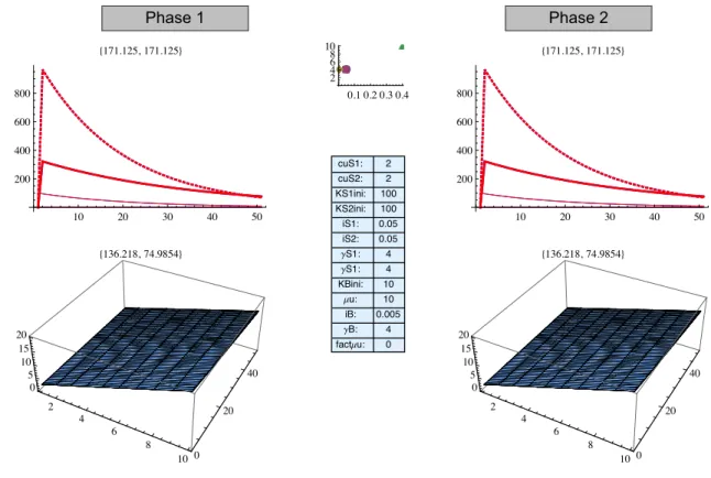
To simulate the history of car industry we distinguish three phases.
In phase 1, the sector is very closed to our reference case #2. The “no obsoleteness” hypothesis becomes a “slow obsoleteness”. In phase 2, the firms focus on the development of new products (K-products) and become strongly project-oriented, putting less emphasis on competence rebuilding and advanced R&D [52]. This can be modeled by a decrease in !S. This has no effect on firm performance in the model (we obtain strictly the same curves and performances)
Figure 3: Automotive case, phases 1 and 2. Graphs on the right handside are obtained with
!S1=!S2=0.05
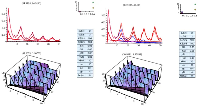
In phase 3, customer becomes more and more sensitive to sustainable development and to the constraints of having a car (costs, traffic jams,…). Car is nolonger a dream. The customer knowledge base hence descreases rapidly, which modeled with iB=0.4. But the customer is still interested in experiments with new forms of cars (Hybrid, Tesla, Car sharing, Autolib, Mobizen,…) hence he keeps a high !B. The consequences are dramatic: firm profits over the time period plunge (from 171.125 to
time 50 cuS1x 2 cuS2x 2 KS1inix 100 KS2inix 100 iS1x 0.05 iS2x 0.05 ΓS1x 4 ΓS2x 4 KBinix 10 Μux iBx 0.005 ΓBx 4 factΜux 10 20 30 40 50 200 400 600 800 2 4 6 8 10 0 20 40 0 5 10 15 20 !171.125, 171.125" !136.218, 74.9854" 10 20 30 40 50 200 400 600 800 2 4 6 8 10 0 20 40 0 5 10 15 20 !0, 456.332" !90.8118, 49.9903" ! ! " " # # $ $ 0.1 0.2 0.3 0.4 2 4 6 8 10 cuS1: 2 cuS2: 2 KS1ini: 100 KS2ini: 100 iS1: 0.05 iS2: 0.05 ΓS1: 4 ΓS1: 4 KBini: 10 Μu: 10 iB: 0.005 ΓB: 4 factΜu: 0 time 50 cuS1x 2 cuS2x 2 KS1inix 100 KS2inix 100 iS1x 0.05 iS2x 0.05 ΓS1x 4 ΓS2x 4 KBinix 10 Μux iBx 0.005 ΓBx 4 factΜux 10 20 30 40 50 200 400 600 800 2 4 6 8 10 0 20 40 0 5 10 15 20 !171.125, 171.125" !136.218, 74.9854" 10 20 30 40 50 200 400 600 800 2 4 6 8 10 0 20 40 0 5 10 15 20 !0, 456.332" !90.8118, 49.9903" ! ! " " # # $ $ 0.1 0.2 0.3 0.4 2 4 6 8 10 cuS1: 2 cuS2: 2 KS1ini: 100 KS2ini: 100 iS1: 0.05 iS2: 0.05 ΓS1: 4 ΓS1: 4 KBini: 10 Μu: 10 iB: 0.005 ΓB: 4 factΜu: 0 Phase 1 Phase 2
page 14 / 28
84,92), aggregated user value plunges too (from 136 to 47), car manufacturer knowledge base follow the same path of slow decrease as in the previous cases but this knowledge is used for cars that don’t attract consumers. In this third phase, U-products are designed and sold, supporting the revival of KB and the associated increase in user value. But the firm lack of learning capacity from the unknown so that it does not learn from these trials. We simulate also an alternative case where one of the two firms (Toyota? Citroën?) actually kept its capacity to learn from the unknown (right hand side on the graph below). This kind of competition has only limited effect on user-value but keep higher profits in the ecosystem (one company becomes a leader with profit = 172 whereas the other declines faster than in the previous case (profit is now 48 instead of 85), but the sum of both profits is 231 vs 170 in the previous case). In this case KS1 remains at a high level.
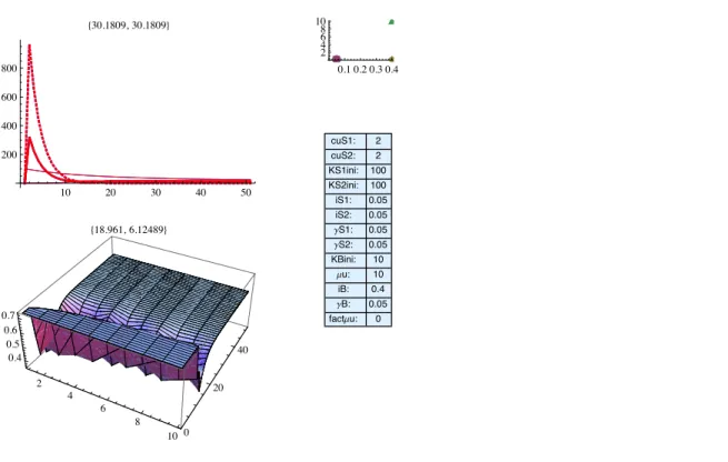
Note that if the consumer renounces to learn from the unknown (gB becomes low), then the whole sector almost disappear (see phase 4 below)
Figure 4: Automotive case, phases 3 and 3’. Graphs on the right hand side are obtained with two
different firms, firm S1 keeps a high !S (!S=1) whereas firm S2 has a low one (!S2=0.05)
time 50 cuS1x 2 cuS2x 2 KS1inix 100 KS2inix 100 iS1x 0.05 iS2x 0.05 ΓS1x 0.05 ΓS2x 0.05 KBinix 10 Μux iBx 0.4 ΓBx 4 factΜux 10 20 30 40 50 200 400 600 800 2 4 6 8 10 0 20 40 0 5 10 15 20 !84.9195, 84.9195" !47.1695, 3.86252" 10 20 30 40 50 200 400 600 800 2 4 6 8 10 0 20 40 0 5 10 !0, 149.699" !20.8999, 3.39165" ! ! " " # # $ $ 0.1 0.2 0.3 0.4 2 4 6 8 10 cuS1: 2 cuS2: 2 KS1ini: 100 KS2ini: 100 iS1: 0.05 iS2: 0.05 ΓS1: 0.05 ΓS1: 0.05 KBini: 10 Μu: 10 iB: 0.4 ΓB: 4 factΜu: 0 time 50 cuS1x cuS2x KS1inix 100 KS2inix 100 iS1x 0.05 iS2x 0.05 ΓS1x 1 ΓS2x 0.05 KBinix 10 Μux iBx 0.4 ΓBx 4 factΜux 10 20 30 40 50 200 400 600 800 2 4 6 8 10 0 20 40 0 5 10 15 20 !172.303, 48.545" !50.8011, 4.93891" 10 20 30 40 50 200 400 600 800 2 4 6 8 10 0 20 40 0 5 10 !0, 149.699" !20.8999, 3.39165" ! ! " " # # $ $ 0.1 0.2 0.3 0.4 2 4 6 8 10 cuS1: 2 cuS2: 2 KS1ini: 100 KS2ini: 100 iS1: 0.05 iS2: 0.05 ΓS1: 1 ΓS2: 0.05 KBini: 10 Μu: 10 iB: 0.4 ΓB: 4 factΜu: 0
page 15 / 28
Figure 5: Automotive case, phase 4. No demand-side learning from the unknown
One can already underline that performance mainly depends on g (more than on i). It is interesting to note that in phase 3’, the “winner” does not make more U-products (actually rather less!).
III.A. Biotech and pharma: simulating an ecology of design firms.
In biotech and pharma case, one begins by simulating the incumbent alone, the incumbent being a classical R&D firm (numbered #2 in the graphs below) (high initial competence, good capitalization (iS-iS2=1%) and relatively low capacity to learn from the unknown (!S2=0.1).
The consumers are demanding (iS=40%, with high capacity to learn from the unknown (!B=4).
We obtain %S2=163, UV=23.
We now introduce a second simulation with a new entrant (S1). S1 has very low initial competence (KS1=1), low capitalization capacity (iS1=40%) and high capacity to learn from
the unknown (!S1=4).
We introduce here one additional notion: the learning efficiency for competence
renewal, !Bj/(iB-iBj) (or !Si/(iS-iSi)). For any Si (respectively Bj) one can compute how much
QU is necessary to maintain K at a constant level K0 over time:
!
KSi,0= KSi,0
(1+ iS " iSi)
+#Si. QU ,Si which gives the equality:
! KSi,0 QU ,Si = "Si (iS# iSi) . This represents the capacity of a firm to transform a certain “quantity” of product into competences. If the learning efficiency is low, a large quantity of products size is required for a certain amount of competence. If the learning efficiency is high a small quantity is enough to maintain stable the competence level.
In our case one can notice that the learning efficiency of S1 and S2 are the same (equal to 10). We see that the incumbent greatly benefits from the new entrant: %S2 increases from 163
to 279 whereas %S1 remains very low (%S1=9). KS2 is not better. The reason for the
time 50 cuS1x cuS2x KS1inix 100 KS2inix 100 iS1x 0.05 iS2x 0.05 ΓS1x 0.05 ΓS2x 0.05 KBinix 10 Μux iBx 0.4 ΓBx 0.05 factΜux 10 20 30 40 50 200 400 600 800 2 4 6 8 10 0 20 40 0.4 0.5 0.6 0.7 !30.1809, 30.1809" !18.961, 6.12489" 10 20 30 40 50 200 400 600 800 2 4 6 8 10 0 20 40 0.4 0.6 0.8 !0, 80.4718" !12.6934, 4.06872" ! ! " " ## $ $ 0.1 0.2 0.3 0.4 2 4 6 8 10 cuS1: 2 cuS2: 2 KS1ini: 100 KS2ini: 100 iS1: 0.05 iS2: 0.05 ΓS1: 0.05 ΓS2: 0.05 KBini: 10 Μu: 10 iB: 0.4 ΓB: 0.05 factΜu: 0
page 16 / 28
performance improvement of S2 is actually the improvement of customer competence. With the new entrant S1, customers’ user value raises from 23 to 48. This increase is due to the quantity of QU designed by S1. Interestingly enough, we can compare this simulation with
another reference: we simulate a case where the incumbent would leave immediately and S1 would be alone on the market (far right on the figure below). In this case S1 has a very good growth (%S1=157) but the user value goes back from 48 to 22 and the overall supply side profit
is 157 instead of 279+9=288.
This simulation illustrates how a diversified ecology of (competing) firms better perform than one incumbent and one start up. It is interesting to note that the high profit level of S2 is finally caused by S1 which raises an interesting issue for profit sharing! This issue is actually caused by the fact that the design of U-products by S1 creates high externalities through customer learning, and S2 benefits from these externalities.
Figure 6: Biotech and pharma, an efficient industrial dynamics based on an ecology of diversified firms.
One can notice that the balance between incumbent and new entrant is fragile. It higly depends on the new entrant learning efficient. We give below an example with a very efficient learner (iS1=4%
-instead of 40% in the previous case-, and !S1=4 like in the previous case; learning efficient raises from
10 to 100). In this case the new entrant outperforms the incumbent (new entrant S1 = 140 ; incumbent S2 = 112). Out[195]= time cuS1x cuS2x KS1inix 1 KS2inix 100 iS1x 0.4 iS2x 0.01 ΓS1x 4 ΓS2x 0.1 KBinix 2 Μux iBx 0.4 ΓBx 4 factΜux 10 20 30 40 50 100 200 300 400 500 600 700 2 4 6 8 10 0 20 40 0 5 10 !8.68681, 279.344" !48.2055, 1.76549" 10 20 30 40 50 50 100 150 200 250 300 2 4 6 8 10 0 20 40 0 2 4 6 !0, 163.355" !22.7544, 0.6178" ! ! " " # # $ $ 0.1 0.2 0.3 0.4 2 4 6 8 10 cuS1: 2 cuS2: 2 KS1ini: 1 KS2ini: 100 iS1: 0.4 iS2: 0.01 ΓS1: 4 ΓS2: 0.1 KBini: 2 Μu: 10 iB: 0.4 ΓB: 4 factΜu: 0 Out[195]= time cuS1x cuS2x KS1inix 1 KS2inix 100 iS1x 0.4 iS2x 0.01 ΓS1x 4 ΓS2x 0.1 KBinix 2 Μux iBx 0.4 ΓBx 4 factΜux 10 20 30 40 50 100 200 300 400 500 600 700 2 4 6 8 10 0 20 40 0 5 10 !8.68681, 279.344" !48.2055, 1.76549" 10 20 30 40 50 50 100 150 200 250 300 2 4 6 8 10 0 20 40 0 2 4 6 !0, 163.355" !22.7544, 0.6178" ! ! " " # # $ $ 0.1 0.2 0.3 0.4 2 4 6 8 10 cuS1: 2 cuS2: 2 KS1ini: 1 KS2ini: 100 iS1: 0.4 iS2: 0.01 ΓS1: 4 ΓS2: 0.1 KBini: 2 Μu: 10 iB: 0.4 ΓB: 4 factΜu: 0 Out[195]= time cuS1x cuS2x KS1inix 100 KS2inix 1 iS1x 0.01 iS2x 0.4 ΓS1x 0.1 ΓS2x 4 KBinix 2 Μux iBx 0.4 ΓBx 4 factΜux 10 20 30 40 50 100 200 300 400 500 600 700 2 4 6 8 10 0 20 40 0 5 10 !279.344, 8.68681" !48.2055, 1.76549" 10 20 30 40 50 100 200 300 400 500 2 4 6 8 10 0 20 40 0 2 4 6 8 !0, 157.474" !22.0509, 0.394555" ! ! ""## $ $ 0.1 0.2 0.3 0.4 2 4 6 8 10 cuS1: 2 cuS2: 2 KS1ini: 100 KS2ini: 1 iS1: 0.01 iS2: 0.4 ΓS1: 0.1 ΓS2: 4 KBini: 2 Μu: 10 iB: 0.4 ΓB: 4 factΜu: 0
page 17 / 28
Figure 7: Biotech and pharma: when an efficient learner outperforms incumbent.
III.A. ITRS: an efficient industrial dynamics based on an organization of collective learning from the unknown.
For ITRS we first build a reference: sellers and buyers are both in a turbulent technological environment, hence iB=iS=40% and this parameter won’t change during the simulation. If !S
and !B are very low, no growth can happen: industrial dynamics is blocked. With a slightly
higher !, growth begins (see figure below, right part). Note that in this simulation, suppliers are suppliers of devices for semiconductor processes and buyers are semiconductors designers and manufacturers.
Figure 8: ITRS reference: low learning from the unknown.
time 50 cuS1x cuS2x KS1inix 1 KS2inix 100 iS1x 0.04 iS2x 0.01 ΓS1x 4 ΓS2x 0.1 KBinix 2 Μux iBx 0.4 ΓBx 4 factΜux 10 20 30 40 50 200 400 600 800 2 4 6 8 10 0 20 40 0 5 10 !139.72, 111.767" !59.8253, 1.5311" 10 20 30 40 50 50 100 150 200 250 300 2 4 6 8 10 0 20 40 0 2 4 6 !0, 163.355" !22.7544, 0.6178" ! ! " " # # $ $ 0.1 0.2 0.3 0.4 2 4 6 8 10 cuS1: 2 cuS2: 2 KS1ini: 1 KS2ini: 100 iS1: 0.04 iS2: 0.01 ΓS1: 4 ΓS2: 0.1 KBini: 2 Μu: 10 iB: 0.4 ΓB: 4 factΜu: 0 Out[223]= time cuS1x cuS2x KS1inix KS2inix 10 iS1x 0.4 iS2x 0.4 ΓS1x 0.1 ΓS2x 0.1 KBinix Μux iBx 0.4 ΓBx 0.1 factΜux 10 20 30 40 50 10 20 30 40 50 2 4 6 8 10 0 20 40 1.22 1.23 1.24 1.25 1.26 !11.5078, 12.7331" !9.37541, 0.0318056" 10 20 30 40 50 10 20 30 40 50 2 4 6 8 10 0 20 40 0.50 0.55 0.60 0.65 !0, 31.9859" !6.29353, 0.0630265" ! ! " " # # $ $ 0.1 0.2 0.3 0.4 2 4 6 8 10 cuS1: 2 cuS2: 2 KS1ini: 1 KS2ini: 10 iS1: 0.4 iS2: 0.4 ΓS1: 0.1 ΓS1: 0.1 KBini: 2 Μu: 10 iB: 0.4 ΓB: 0.1 factΜu: 0 Out[223]= time cuS1x cuS2x KS1inix KS2inix 10 iS1x 0.4 iS2x 0.4 ΓS1x 0.5 ΓS2x 0.5 KBinix Μux iBx 0.4 ΓBx 0.5 factΜux 10 20 30 40 50 10 20 30 40 50 2 4 6 8 10 0 20 40 1 2 3 4 !14.9447, 18.1349" !9.70111, 0.117862" 10 20 30 40 50 10 20 30 40 50 2 4 6 8 10 0 20 40 0.5 1.0 1.5 2.0 !0, 40.0694" !6.45725, 0.0958179" ! ! " " # # $ $ 0.1 0.2 0.3 0.4 2 4 6 8 10 cuS1: 2 cuS2: 2 KS1ini: 1 KS2ini: 10 iS1: 0.4 iS2: 0.4 ΓS1: 0.5 ΓS1: 0.5 KBini: 2 Μu: 10 iB: 0.4 ΓB: 0.5 factΜu: 0
page 18 / 28
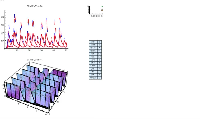
We now simulate the role of ITRS: ITRS organizes knowledge sharing on the alternatives for the future, based on experiments and trials made all over the world. Hence ITRS increases the capacity to transform experiments into knowledge. We simulate ITRS as a global increase of !: !S=!B=4.
In this case profits raise from 15 to 90 for each supplier and user value raises from 10 to 51.
Figure 9: ITRS simulation
We also try to model alternative organizations, that are often discussed in such consortia organization. One could have expected knowledge sharing between sellers (oligopolistic organization). We simulate that process with !S high and !B low (see below). The profits fall
from 90 to 28 and user value from 51 to 16. This shift provokes an increase in KS and in
U-products. Conversely one could have imagined a consortium of buyers (oligopsony). In this
case profit fall from 90 to 41 and user value from 51 to 26. This shift provokes a decrease in KS and an increase in U-products. Hence oligopoly and oligopsony tend to perform lower.
This lower performance is related to an increase in U-products. In case of demand-side low learning, supply side “compensates” demand side low learning by an increase of knowledge production KS. This shows that high quantity of U-products and high level of competences are
not necessary a symptom of well performing sector: it can also be a symptom of poor performance in learning from the unknown.
Out[223]= time cuS1x cuS2x KS1inix KS2inix 10 iS1x 0.4 iS2x 0.4 ΓS1x 5 ΓS2x 5 KBinix Μux iBx 0.4 ΓBx 5 factΜux 10 20 30 40 50 100 200 300 400 2 4 6 8 10 0 20 40 0 5 10 15 !90.2384, 95.7762" !51.4714, 3.75444" 10 20 30 40 50 50 100 150 200 250 2 4 6 8 10 0 20 40 0 2 4 6 8 !0, 133.902" !18.7152, 0.6331" ! ! " " # # $ $ 0.1 0.2 0.3 0.4 2 4 6 8 10 cuS1: 2 cuS2: 2 KS1ini: 1 KS2ini: 10 iS1: 0.4 iS2: 0.4 ΓS1: 5 ΓS1: 5 KBini: 2 Μu: 10 iB: 0.4 ΓB: 5 factΜu: 0
page 19 / 28
Figure 10: ITRS alternatives: oligopoly and oligopsony provoke an “over production” of knowledge and U-products.
III.A. Orphan innovation
We simulate here suppliers with an efficient learning in a turbulent sector (iS=10%, !S=4,
learning efficiency = 40), with poorly efficient customers (iB=10%, !B=0.01, learning efficient
=0.1). In this case the growth remain very limited (%S1=%S2=18 and user value = 13) but we
see a very important increase in KS. Hence that lack of demand-side learning from the
unknown is a critical factor: even a very efficient firm on the supply-side won’t be able to launch industrial growth (see the second example below with learning efficiency = 80; we get %S1=%S2=21 and user value = 15).
Figure 11: Orphan innovation: the effect of low learning from the unknown.
Out[223]= time cuS1x cuS2x KS1inix KS2inix 10 iS1x 0.4 iS2x 0.4 ΓS1x 5 ΓS2x 5 KBinix Μux iBx 0.4 ΓBx 0.5 factΜux 10 20 30 40 50 50 100 150 2 4 6 8 10 0 20 40 1 2 3 4 !28.1329, 30.0378" !16.4828, 0.696816" 10 20 30 40 50 20 40 60 80 2 4 6 8 10 0 20 40 0.5 1.0 1.5 2.0 !0, 47.6801" !7.04733, 0.193223" ! ! " " # # $ $ 0.1 0.2 0.3 0.4 2 4 6 8 10 cuS1: 2 cuS2: 2 KS1ini: 1 KS2ini: 10 iS1: 0.4 iS2: 0.4 ΓS1: 5 ΓS1: 5 KBini: 2 Μu: 10 iB: 0.4 ΓB: 0.5 factΜu: 0 Out[223]= time cuS1x cuS2x KS1inix KS2inix 10 iS1x 0.4 iS2x 0.4 ΓS1x 0.5 ΓS2x 0.5 KBinix Μux iBx 0.4 ΓBx 5 factΜux 10 20 30 40 50 50 100 150 2 4 6 8 10 0 20 40 0 5 10 15 !41.1048, 55.3142" !26.1094, 1.63512" 10 20 30 40 50 20 40 60 80 100 2 4 6 8 10 0 20 40 0 2 4 6 8 !0, 78.3433" !11.1414, 0.283841" ! ! " " # # $ $ 0.1 0.2 0.3 0.4 2 4 6 8 10 cuS1: 2 cuS2: 2 KS1ini: 1 KS2ini: 10 iS1: 0.4 iS2: 0.4 ΓS1: 0.5 ΓS1: 0.5 KBini: 2 Μu: 10 iB: 0.4 ΓB: 5 factΜu: 0 In[195]:= time cuS1x cuS2x KS1inix 1 KS2inix 1 iS1x 0.1 iS2x 0.1 ΓS1x 4 ΓS2x 4 KBinix 2 Μux iBx 0.1 ΓBx 0.01 factΜux 10 20 30 40 50 50 100 150 200 250 300 350 2 4 6 8 10 0 20 40 0.5 1.0 1.5 !18.0321, 18.0321" !13.4041, 3.61852" 10 20 30 40 50 100 200 300 400 500 2 4 6 8 10 0 20 40 0.5 1.0 1.5 !0, 47.2676" !8.91337, 2.36946" ! ! " " # # $ $ 0.1 0.2 0.3 0.4 2 4 6 8 10 cuS1: 2 cuS2: 2 KS1ini: 1 KS2ini: 1 iS1: 0.1 iS2: 0.1 ΓS1: 4 ΓS1: 4 KBini: 2 Μu: 10 iB: 0.1 ΓB: 0.01 factΜu: 0 Out[184]= time cuS1x cuS2x KS1inix 100 KS2inix 100 iS1x 0.05 iS2x 0.05 ΓS1x 4 ΓS2x 4 KBinix 2 Μux iBx 0.1 ΓBx 0.01 factΜux 10 20 30 40 50 100 200 300 400 500 2 4 6 8 10 0 20 40 0.5 1.0 1.5 !20.7136, 20.7136" !15.2886, 4.88419" 10 20 30 40 50 200 400 600 800 2 4 6 8 10 0 20 40 0.0 0.5 1.0 1.5 !0, 55.7053" !10.388, 3.39363" ! ! " " # # $ $ 0.1 0.2 0.3 0.4 2 4 6 8 10 cuS1: 2 cuS2: 2 KS1ini: 100 KS2ini: 100 iS1: 0.05 iS2: 0.05 ΓS1: 4 ΓS1: 4 KBini: 2 Μu: 10 iB: 0.1 ΓB: 0.01 factΜu: 0
page 20 / 28
We then test two strategies to get growth in such a situation. Either support the increase in iB (to 0,1%), by supporting the capitalization on the technology (teaching, handbook,…), without increasing !B (stay at 0.01). Or increase !B (to 1) without increasing iB (at 10%). This
second strategy consists for instance in organizing knowledge sharing on recent trials and prototypes. We keep an equal learning efficiency between both cases (10 in both cases).
It is interesting to note that resulting industrial dynamics are strongly different: in the case of “support to memorization” appears a segmentation between a vast majority of users who are satisfied with the K-products and a small minority (niche) which regularly asks for U-products. This minority provokes a regular updates of supply-side knowledge and hence K-products. Suppliers offer regularly K-products and simultaneously a small quantity of U-products. In the case of “support to learning from the unknown” appear cycles with phases where suppliers design only K-products and all customers segments are satisfied and phases where one or several segments are unsatisfied so that suppliers offer simultaneously K- and U-innovation. All market segments have the opportunity to learn from the unknown.
Figure 12: Orphan innovation: support memorization vs support demand-side learning from the unknown.
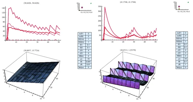
To a certain extent both strategies perform equally well (see figure below: support of memorization get %S1=%S2= 39 and user value = 31; support for learning gets %S1=%S2= 41 and
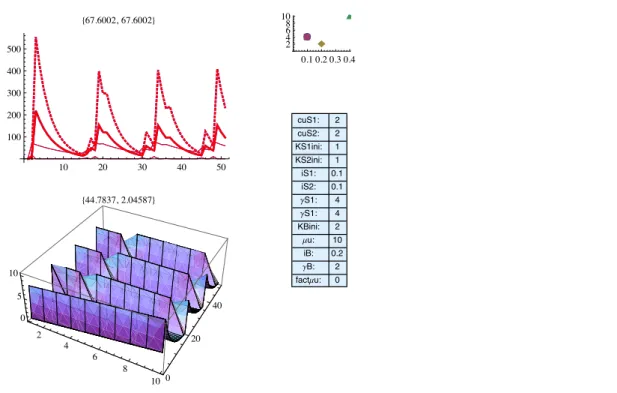
user value = 30). But the growth dynamics are strongly different with a slow decrease in the first case and innovation waves and new product generation in the second. This is clear if one one increases !B to 2 while keeping the learning efficiency constant to 10 (ie iB=20%, ie one
increases iB!), then we get a much higher growth, in profit (%S1=%S2= 68) and in user value
(=45). Out[197]= time cuS1x cuS2x KS1inix 1 KS2inix 1 iS1x 0.1 iS2x 0.1 ΓS1x 4 ΓS2x 4 KBinix 2 Μux iBx 0.001 ΓBx 0.01 factΜux 10 20 30 40 50 20 40 60 80 100 120 140 2 4 6 8 10 0 20 40 0 1 2 3 4 !38.6426, 38.6426" !30.8837, 15.7724" 10 20 30 40 50 20 40 60 80 100 120 140 2 4 6 8 10 0 20 40 0 1 2 3 4 !0, 109.737" !21.9258, 11.4503" ! ! " " # # $ $ 0.1 0.2 0.3 0.4 2 4 6 8 10 cuS1: 2 cuS2: 2 KS1ini: 1 KS2ini: 1 iS1: 0.1 iS2: 0.1 ΓS1: 4 ΓS1: 4 KBini: 2 Μu: 10 iB: 0.001 ΓB: 0.01 factΜu: 0 In[196]:= time cuS1x cuS2x KS1inix 1 KS2inix 1 iS1x 0.1 iS2x 0.1 ΓS1x 4 ΓS2x 4 KBinix 2 Μux iBx 0.1 ΓBx 1 factΜux 10 20 30 40 50 50 100 150 200 250 300 350 2 4 6 8 10 0 20 40 0 2 4 6 !41.3746, 41.3746" !30.0713, 1.25379" 10 20 30 40 50 50 100 150 200 2 4 6 8 10 0 20 40 1 2 3 4 5 !0, 72.3094" !13.1577, 1.29753" ! ! " " # # $ $ 0.1 0.2 0.3 0.4 2 4 6 8 10 cuS1: 2 cuS2: 2 KS1ini: 1 KS2ini: 1 iS1: 0.1 iS2: 0.1 ΓS1: 4 ΓS1: 4 KBini: 2 Μu: 10 iB: 0.1 ΓB: 1 factΜu: 0
page 21 / 28
Figure 13: Orphan innovation: support to demand-side learning from the unknown can outperform support to demand-side memorization.
IV. Research proposals and discussion: organizing learning from
the unknown as a common good supporting sectoral performance.
To analyse industrial dynamics in Schumpeterian development situations, we built a model of economic growth based on design functions. This model endogeneizes learning and novelty creation, in so far as learning occurs through the design of novelty and novelty occurs when existing products are obsolete, either from seller or from buyer point of view. This model brings four main results for industrial growth that we will first present. We will then show how I can pave the way to a general model of industrial sector and to new research questions.
IV.A. Main results of the simulations: the role of learning from the unknown in industrial growth
The main results of the model are the following:
1- Revise performance (efficiency) criteria. Growth in profit and in user-value is based on limited and efficient novelty creation. For given sectoral conditions (obsoleteness, number of players, initial knowledge level,…) some suboptimal growth pathes show too much novelty and too much knowledge production. There can be hogh knowledge production and frequent U-products design without growth and, conversely, growth through innovation with limited knowledge production and limited U-products design. This suggests to analyze knowledge-based economy and innovation-based growth as an “economy” (in the sense of economize, sparing) of knowledge and novelty, ie growth through limited novelty and knowledge production. An “optimal” growth trajectory is not related to maximal knowledge production and
time 50 cuS1x cuS2x KS1inix 1 KS2inix 1 iS1x 0.1 iS2x 0.1 ΓS1x 4 ΓS2x 4 KBinix 2 Μux iBx 0.2 ΓBx 2 factΜux 10 20 30 40 50 100 200 300 400 500 2 4 6 8 10 0 20 40 0 5 10 !67.6002, 67.6002" !44.7837, 2.04587" 10 20 30 40 50 50 100 150 200 250 300 2 4 6 8 10 0 20 40 0 2 4 6 !0, 102.068" !16.9565, 0.382041" ! ! " " ## $ $ 0.1 0.2 0.3 0.4 2 4 6 8 10 cuS1: 2 cuS2: 2 KS1ini: 1 KS2ini: 1 iS1: 0.1 iS2: 0.1 ΓS1: 4 ΓS1: 4 KBini: 2 Μu: 10 iB: 0.2 ΓB: 2 factΜu: 0
page 22 / 28
U-products launches but to a “balance” between U-products and K-products, ie innovative design and rule-based design.
Note that we could favor different measures of growth but our model suggests measuring growth at the industry level by considering profits from all suppliers and user value aggregated at the demand-side level.
2- Knowledge management criteria. In our model, growth is mainly related to knowledge management criteria. In our model, knowledge “management”’ can take several forms: initial knowledge level, knowledge “capitalization” (slow i) and learning from unknown products (high !). Simulations underline following features: Growth performance of an overall economy depends hardly on initial competence level (initial competence level has a strong influence only in cases of non unlearning and non-obsoleteness industrial dynamics!); it depends much more on learning capacity by S and B. Moreover it depends less on “long term” memorization (capitalization) than on learning from the unknown. Learning from the unknown is of course critical in high velocity markets (like ITRS) where long term memory (or capitalization) is of course difficult. In case of “dynamic markets”, learning from
the unknown has a much stronger effect on growth than initial knowledge and “long term” memory. This result can enrich the debate on core competences and
dynamic capability of the firm: according to our model, as soon as the industrial sector is slightly changing (iB or iS slightly positive) suppliers and buyers should favor
“dynamic capabilities” as long as these capabilities are really targeting learning from the unknown.
Moreover, low iB can even have negative effects on the demand-side, where it is often
even better to have a high iB (see automotive or orphan innovation).
3- Learning from the unknown as a common good: Learning through the unknown depends on individual firm performance but the effort of one side has deep effects on all sides. There are strong externalities with U-type innovation, since customer learning is worth for the whole economy. Conversely profits and user value from K-products have no externalities. In particular “good” ecosystem not only depend on seller but also a) on buyer: it might be necessary to organize for increasing !B and/or to organize “low iB” (orphan innovation) or even high iB (better than rule-based!)); b)
on the variety of product providers (synergy between new entrant and incumbents. Note that such strategies are all the more difficult that customers can often decide to buy something different!, they are not tight to one specific type of product. Hence growth depends on population ecology or/and on customer learning capacities. This calls for a kind of management of the externalities through which firms should cope with their competitors (keep a balanced ecosystem) and firms should also cope with customer learning. Hence our proposition: learning from the unknown appears as a
common good.
Note that this common good raises completely different issues for regulation: consortia appear less as monopolistic organization trying to control prices than organizations that should be concerned more by learning from the unknown than pricing
Consortia and standardization committee are often represented as competing organizations. In our model, two types of common good can be managed: standardization committees actually tend to decrease iS by capitalizing on existing
rules; private consortia might appear as complementary to this task: they tend to increase !B by supporting experience sharing.