Any correspondence concerning this service should be sent to the repository
administrator: [email protected]
O
pen
A
rchive
T
OULOUSE
A
rchive
O
uverte (
OATAO
)
OATAO is an open access repository that collects the work of Toulouse researchers and
makes it freely available over the web where possible.
This is an author-deposited version published in:
http://oatao.univ-toulouse.fr/
Eprints ID: 17660
To cite this version:
Paroissien, Eric and Gaubert, Frédéric and Da Veiga, Anthony and
Lachaud, Frédéric Elasto-Plastic Analysis of Bonded Joints with Macro-Elements. (2013)
Journal of Adhesion Science and Technology, vol. 27 (n° 13). pp. 1464-1498. ISSN
0169-4243
1
Elasto-Plastic Analysis of Bonded Joints with Macro-Elements
E. PAROISSIEN1,*, F. GAUBERT1, A. DA VEIGA1,F. LACHAUD2
1SOGETI HIGH TECH, Parc le Millénaire - Bât A1, Avenue de l’Escadrille Normandie Niemen, 31700 BLAGNAC, FRANCE
2Institut Clément Ader, ISAE/DMSM, Campus ENSICA, 1 Place Emile Blouin, 31500 TOULOUSE
Running Head: Elasto-Plastic Analysis of Bonded Joints
*To whom correspondence should be addressed: Tel. +33534362684, Fax. +33534362626, E-mail: [email protected]
2 Abstract – The Finite Element (FE) method could be able to address the stress analysis of bonded joints. Nevertheless, analyses based on FE models are mainly computationally cost expensive and it would be profitable to develop simplified approaches, enabling extensive parametric studies. Firstly, a 1D-bar and 1D-beam simplified models for the bonded joint stress analysis, assuming a linear elastic adhesive material, are presented. These models derive from an approach, inspired by the finite element (FE) method using a formulation based on a 4-node macro-element, which is able to simulate an entire bonded overlap. Moreover, a linear shear stress variation in the adherend thickness is included in the formulation. Secondly, a numerical procedure is then presented to introduce into both models an elasto-plastic adhesive material behavior, while keeping the previous linear elastic formulation. Finally, assuming an elastic perfectly plastic adhesive material behavior, the results produced by simplified models are compared with the results predicted by FE using 1D-bar, plane stress and 3D models. Good agreements are shown.
keywords: bonded joint, single-lap shear, non-linear material adhesive, Finite Element method, analytical formulation, macro-element
NOMENCLATURE AND UNITS
Aj extensional stiffness (N) of the adherend j
Bj extensional and bending coupling stiffness (N.mm) of the adherend j Dj bending stiffness (N.mm2) of the adherend j
Ej Young’s modulus (MPa) of the adherend j E Young’s modulus (MPa) of in the adhesive F vector of forces
G Coulomb’s modulus (MPa) of the adhesive Gj Coulomb’s modulus (MPa) of the adherend j K stiffness matrix
3 KBBa stiffness matrix of the Bonded-Bars element
KBBe stiffness matrix of the Bonded-Beams element L length (mm) of the overlap
Mj moment (N.mm) in the adherend j around the z direction Nj force (N) in the adherend j in the x direction
Q nodal normal force (N) applied to the node in the x direction ( = i,j,k,l)
R nodal shear force (N) applied to the node in the y direction ( = i,j,k,l)
S nodal bending moment (N.mm) applied to the node around the z direction ( =
i,j,k,l)
S adhesive peel stress (MPa) T adhesive shear stress (MPa) U vector of displacements
Vj shear force (N) in the adherend j in the y direction
b width (mm) of the adherends (lateral pitch between two rows of fasteners) e thickness (mm) of the adhesive
ej thickness (mm) of the adherend j
f force (N) applied to the joint in the x direction
lj length (mm) of the beam outside the overlap of the adherend j n number of macro-elements
uj displacement (mm) of the adherend j in the x direction
ua displacement (mm) of the node a in the x direction (a = i,j,k,l) wj displacement (mm) of the adherend j in the y direction
wa displacement (mm) of the node a in the y direction (a = i,j,k,l)
length (mm) of a macro-element
j angular displacement (rad) of the adherend j around the z direction
a angular displacement (rad) of the node a around the z direction (a = i,j,k,l) (x,y,z) direct orthonormal base
4 1. INTRODUCTION
1.1. Context
In the frame of the structural component design, bonding can be considered as a suitable assembly method or an attractive complement to conventional methods such as bolting or riveting. Bonding offers the possibility of joining without damaging various materials, like plastics or metals, as well as allowing for various combinations of materials. This first advantage is reinforced by a large choice of adhesive families and by the possibility to formulate adhesives, designed to best meet the joint specifications, while optimizing the structure. Bonding allows mainly for mass benefits with regard to other mechanical fastening methods, since the materials volume required is reduced to sustain static or fatigue loads. The Finite Element (FE) method could be able to address the stress analysis of bonded joints. Nevertheless, analyses based on FE models are mainly computationally cost expensive and it would be profitable to develop simplified approaches, enabling extensive parametric studies. The study, presented in this paper, takes place in this context. As highlighted in several literature surveys [1-3], a large number of simplified approaches for the stress analysis of bonded joints exist in the open literature.
1.2. Objective
The objective of this paper is to present a simplified approach for the stress analysis of bonded joints, taking into account an elasto-plastic adhesive material behavior. This topic was already addressed by several authors (e.g.: [4-11]), leading to the presentation of semi-analytical solutions. Indeed, in order to enlarge the application field of models, the number of simplifying hypotheses has to be restricted. The resolution of the complete set of governing equations, derived from the restricted hypotheses, requires then the development of dedicated procedures, even under the assumption of linear elastic
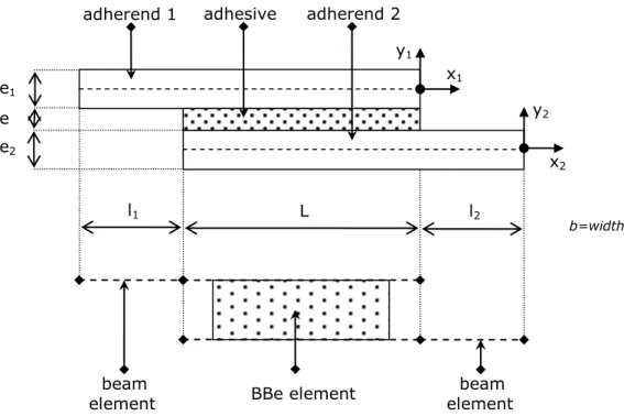
5 material behaviors. In this paper, a restricted number of simplifying hypotheses is similarly under consideration, so that closed-form solutions are not provided. However, an original procedure allowing for the resolution is presented. The simplified approach, presented in this paper, consists then in an iterative resolution scheme, using a simplified linear elastic method for the stress analysis of bonded joints. The simplified linear elastic method is based on the analytical formulation of a 4-node macro-element, in the frame of both 1D-bar and 1D-beam analyses. It is then exemplified on the single-lap bonded joint configuration (see Fig. 1 and Tab. 1).
1.3. Overview of the simplified linear elastic method
The simplified linear elastic method, originally presented in [12, 13], is inspired by the FE method and allows for the resolution of the set of governing differential equations. The displacements and forces in the adherends, as well as the adhesive stresses are then computed. The method consists in meshing the structure in elements. A full bonded overlap is meshed by a unique 4-node macro-element, which is specially formulated. This macro-element is called bonded-bars (BBa) or bonded-beams (BBe), depending on the 1D analysis frame. According to the classical FE rules, the stiffness matrix of the structure – termed K – is assembled and the selected boundary conditions are applied. The minimization of the total potential energy leads to find the vector of nodal displacements U such F=KU, where F is the vector of nodal forces. This approach based on macro-elements takes advantage of the flexibility of FE method. Indeed, by employing a macro-element as an elementary brick, it offers the possibility to simulate complex structures involving single-lap bonded joints [14]. Only simple manipulations on the stiffness matrix of the structure are required. An approach for the simulation of hybrid (bolted/bonded) joints can consist in employing macro-elements for the bonded parts and springs for the fasteners [12, 13]. Finally, various mechanical or thermal loadings could be taken into account, through the vector of nodal forces.
6 1.4. Overview of the paper
The mechanical and geometrical parameters are free; in particular, unbalanced configurations can be addressed. In the 1D-bar (1D-beam) frame, the adherends are simulated as linear elastic bars (as laminated linear elastic Euler-Bernoulli beams), while the adhesive layer simulation consists in continuously distributed linear or non-linear shear springs (in continuously distributed linear or non-linear shear and peeling springs). The adhesive layer thickness is assumed constant along the overlap.
BBa and BBe elements were previously developed [12, 13, 15]. Nevertheless, they do not take into account the shear stress in the adherends. The first part of the paper is then dedicated to the detailed presentation of the formulation of 1D-bar and 1D-beam macro-elements, including a linear variation of shear stress in the adherends, according to the approach of Tsai et al. [16]. Elements of validation are presented, by showing that under the same hypotheses as the Tsai et al. model, the same results are obtained. Secondly, the introduction of an iterative resolution scheme is presented, to take into account an elasto-plastic adhesive material behavior. The projection algorithm with elastic matrix is employed for the numerical resolution. Thirdly, a 1D-bar FE model, involving bar elements and shear springs, is developed as a numerical image of the simplified 1D-bar model. Besides, a plane stress (PS) and 3D FE models are developed to assess the performances of the simplified 1D-beam model.
2. LINEAR ELASTIC 1D-BAR AND 1D-BEAM MODELS
2.1. 1D-Bar model
2.1.1. Formulation of the BBa element
2.1.1.1 – Hypotheses. The model is based on the following hypotheses: (i) the thickness of the adhesive layer is constant along the overlap, (ii) the adherends are
7 linear elastic materials simulated as bars, (iii) the adhesive layer is simulated by an infinite number of linear elastic shear springs linking both adherends, and possibly (iv) the adherend shear stress varies linearly with the adherend thickness.
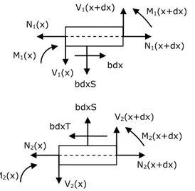
2.1.1.2. Governing Equations. The local equilibrium of both adherends (see Fig. 2) and the linear elastic material behaviors provide the following set of governing equations:
e u u G T j dx du be E N bT dx dN j j j j j j 1 2 2 , 1 ) 1 (
(1)
where e is the adhesive thickness, e1 (e2) the thickness of the adherend 1 (2), b the
width, G the adhesive shear modulus, E1 (E2) the Young’s modulus of the adherend 1 (2), N1 (N2) the normal force in the adherend 1 (2) and T is the adhesive shear stress. The
displacements u1(x) (u2(x)) are the normal displacements of points located at the
abscissa x on the neutral line of adherend 1 (2) before deformation (see Fig. 3).
2.2.1.3. Stiffness matrix of the BBa element. The system of equations (1) leads to the following system of linear differential equations:
0 u u e eE G dx u d 0 u u e eE G dx u d 1 2 2 2 2 1 2 1 2 1 1 2 1 2 (2)8
2 1 x 4 x 3 2 2 1 x 4 x 3 1 c x c e c e c 5 . 0 u c x c e c e c 5 . 0 u with: 1 1 2 2 2 2 2 1 1 2 2 E e 1 E e 1 e G E e 1 E e 1 e G 1 1 (3) where c1, c2, c3and c4 are integration constants.The boundary conditions at both extremities of the BBa element, in terms of displacements, lead to expressions for the integration constants, as functions of nodal displacements ui, uj, uk and ul (see Fig. 3):
) ( sh 2 e u u u u c ) ( sh 2 u u e u u c u u c u u u u c u u u u u 0 u u 0 u i j k l 4 k l i j 3 i j 2 i j k l 1 l 1 k 1 j 2 i 1 (4)
where is the length of the BBa element.
The linear elastic behavior of adherends allows then for the expression of adherend normal forces as a function of nodal displacements, through the integration constants (equation (1.1) and equation (3)):
3 x 1 x 2 2 2 2 3 x 2 x 1 1 1 1 c e c e c e E b 5 . 0 N c e c e c e E b 5 . 0 N (5)
In the same way, the adhesive shear stress is then computed with equation (1.3) as:
1 x 2 x 3
1 1e c e c e c E b 5 . 0 T (6)
9 The nodal forces Qi, Qj, Qk, Ql, which represent the action of nodes i, j, k, l respectively
on the BBa element (see Fig. 3), can be expressed as functions of nodal displacements (equation (5)):
3 1 2 2 2 l 3 2 1 1 1 k 3 1 2 2 2 j 3 2 1 1 1 i 2 l 1 k 2 j 1 i c e c e c e E b 5 . 0 Q c e c e c e E b 5 . 0 Q c c c e E b 5 . 0 Q c c c e E b 5 . 0 Q N Q N Q 0 N Q 0 N Q (7)The stiffness matrix of the BBa element is defined by:
l k j i l k j i ll lk lj li kl kk kj ki jl jk jj ji il ik ij ii Q Q Q Q u u u u k k k k k k k k k k k k k k k k
(8)
where:l
k
j
i
u
Q
k
,
,
,
,
,
(9)Finally, the stiffness matrix of the BBa element, named KBBa, can be written as:
(10)
10
1 1 2 2 1 1 2 2 2 2 1 1 2 2 1 1 1 1 2 2 1 1 2 2 2 2 1 1 2 2 1 1 2 2 BBa e E e E th th 1 e E e E sh 1 sh th 1 e E e E th 1 sh e E e E sh e E e E sh 1 sh e E e E th th 1 1 sh e E e E sh th 1 e E e E th 2 b e E K 2.1.1.4. Considering the shear stress in the adherends. Following [16], a linear distribution of the shear stress, named T1 (T2), in the thickness of the adherend 1 (2) is
assumed:
, j 1,2 e y 2 1 1 2 T T j j j j (11)
where y1 and y2 are local y-axis, as defined in Fig. 1.
The shear deformation, named 1 (2), in the adherend 1 (2) is then given by:
, j 1,2 y ) y , x ( u G T e y 2 1 1 2 1 G T j j j j j j j j j j (12)where G1 (G2) is the shear modulus of the adherend 1 (2).
The integration of equation (12) allows for the expression of the normal displacements of adherends, as functions of x and yj:
2 2 2 2 2 2 2 2 1 1 2 1 1 1 1 1 y 0 j j j 1 j j y e y G 2 T ) 0 , x ( u ) y , x ( u y e y G 2 T ) 0 , x ( u ) y , x ( u dy G T ) 0 , x ( u y , x u j (13)11 The normal forces in the adherends are then deduced:
G dTdx e 3 1 dx ) 0 , x ( du E be N dx dT G e 3 1 dx ) 0 , x ( du E be N dy x ) y , x ( u E b N 2 1 2 2 2 2 2 1 1 1 1 1 2 e 2 e j j j j j j j (14)But, by noticing that the average value of the normal displacement on the adherend thickness is given by:
2 2 2 2 1 1 1 1 2 e 2 e j j j j j G T e 3 1 ) 0 , x ( u u G T e 3 1 ) 0 , x ( u u dy ) y , x ( u e 1 u j j (15)the normal forces in the adherends and the adhesive shear stress can be written as:
e u u G T dx u d E be N 1 2 j j j j with 2 2 1 1 2 2 3 1 1 G e G e e G G G (16)
Finally, to take into account a linear variation of the shear stress in the adherends, the resolution consists in substituting G by G and uj by uj, in the formulation, which does not consider any shear stress in the adherends.
2.1.2. Assembly and validation on the exemplified single-lap joint. The single-lap bonded joint is meshed as following: (i) the overlap is meshed which 1 BBa element, (ii) each adherend outside the overlap is meshed with 1 bar element. This mesh leads to a total number of 6 nodes (see Fig. 4).
12 The stiffness matrix of the single-lap joint is then assembled, according to the classical FE rules, through the stiffness matrices of each element. The stiffness matrix for the bar element, named Kbar, is:
2 , 1 j , 1 1 1 1 l b e E K j j j bar (17)
where l1 (l2) is the length of the bar outside the overlap of the adherend 1 (2).
Following the classical FE rules, the boundary conditions are then applied to the single-lap bonded joint, which is clamped at one extremity and free to move at the other one, where a force f=10 N is applied (see Fig. 4). A total number of degrees of freedom (DoF) equal to 5 is then involved. The resolution consists then in inverting a 5x5 linear system. The adhesive stress distribution predicted by [16] is compared to the model predictions for the single-lap bonded joint defined in Fig. 1 and Tab. 1. The superimposition of curves shown in Fig. 5, allows for the conclusion that the same hypotheses lead to the same results.
2.2. 1D-beam model
2.2.1. Formulation of the BBe element
2.2.1.1. Hypotheses. The model is based on the following hypotheses: (i) the thickness of the adhesive layer is constant along the overlap, (ii) the adherends are simulated by linear elastic Euler-Bernoulli laminated beams, (iii) the adhesive layer is simulated by an infinite number of elastic shear and transverse springs linking both adherends, and possibly (iv), the adherend shear stress varies linearly with the adherend thickness.
13 2.2.1.2. Governing equations. The local equilibrium of both adherends (see Fig. 6) leads to the following system of six equations:
, j 1,2 0 bT 2 e V dx dM S 1 bdx dV T 1 bdx dN j i j 1 j j j j (18)where S is the adhesive peeling stress, V1 (V2) the shear force in the adherend 1 (2) and M1 (M2) the bending moment in the adherend 1 (2).
This local equilibrium is the one derived and employed by Goland and Reissner [17] in their classical theory. Furthermore, considering a possible extensional and bending coupling stiffness in the adherends, the constitutive equations are expressed as:
2 , 1 j , dx dw dx w d D dx du B M dx w d B dx du A N j j 2 j 2 j j j j 2 j 2 j j j j (19)
with Aj the extensional stiffness, Bj the coupling stiffness, and Dj the bending stiffness.
It is assumed that j=Aj2-BjDj is not equal to zero. The adhesive is considered as linear
elastic and is simulated by an infinite number of shear and transverse normal springs. The adhesive shear stress and the adhesive peeling stress are then expressed by:
14 e w w E S e e 2 1 e 2 1 u u G T 2 1 2 2 1 1 1 2 (20)
where E is the Young’s modulus of the adhesive, w1 (w2) the deflection of the adherend 1
(2) and 1 (2) the bending angle of the adherend 1 (2).
2.2.1.3. Stiffness Matrix of the BBe element.
System of differential equations in terms of adhesive stresses. The equation (19) is written as: 2 , 1 j , N B M A dx w d M B N D dx du j j j j j 2 j 2 j j j j j j (21)
By combining equations (18), (20), (21), the following linear differential equation system, in terms of adhesive stresses, is obtained:
dx dT k S k dx S d S k dx dT k dx T d 3 4 4 4 2 1 3 3 (22) where:
15 2 2 1 1 4 2 2 1 1 2 2 2 1 1 1 3 2 2 1 1 2 2 2 1 1 1 2 2 2 2 1 1 1 2 2 2 2 2 2 1 2 1 1 1 1 1 A A e Eb k B B 2 A e 2 A e e Eb k B B 2 A e 2 A e e Gb k B e B e D 4 e A 1 D D 4 e A 1 D e Gb k (23)
The system of differential equations (22) can be uncoupled by differentiation and linear combination as: 0 ) ( 0 ) ( 4 1 3 2 2 2 4 4 4 1 6 6 4 1 3 2 2 2 4 4 4 1 6 6 k k k k T dx T d k dx T d k dx T d dx d k k k k S dx S d k dx S d k dx S d (24)
This system is solved and the adhesive shear and peeling stresses are thus written as (see Appendix A):
7 6 5 4 3 2 1 6 5 4 3 2 1 ) cos( ) sin( ) cos( ) sin( ) ( ) cos( ) sin( ) cos( ) sin( ) ( K e K e K tx e K tx e K tx e K tx e K x T e K e K tx e K tx e K tx e K tx e K x S rx rx sx sx sx sx rx rx sx sx sx sx
(25)
There are then 13 integration constants. However, by introducing these previous expressions of adhesive stresses in equation (22), the integration constants of the adhesive peeling stress appear linked to those of adhesive shear stress as:
16 6 3 6 2 2 1 6 5 3 5 2 1 2 5 4 1 3 2 2 2 1 2 2 3 2 1 2 2 4 4 2 3 1 4 2 1 2 2 3 2 1 2 2 3 2 1 1 2 2 2 1 2 2 1 2 1 2 2 2 2 2 1 1 2 2 1 2 2 1 2 1 2 2 1 K K k ) r k ( r K K K k ) k r ( r K K K K k ) k s t 3 ( s K k ) k t s 3 ( t K K K K k ) k s 3 t ( t K k ) k s t 3 ( s K K K K k ) k t 3 s ( s K k ) k t s 3 ( t K K K K k ) k s 3 t ( t K k ) k t 3 s ( s K (26)
Finally, 7 independent integration constants are remaining: K1 to K7.
Nodal displacements and forces. The determination of the stiffness matrix of BBe element requires the determination of nodal displacements and forces (see Fig. 7). Following the resolution scheme in [18], the idea is to express the displacements and the forces in the adherends, as a function of the stress adhesives and of their derivatives. The computation is fully detailed in Appendix B. It is shown that a total number of 12 integration constants is finally involved: K1 to K7, J1 to J3 and J5 to J6. The displacements
17 6 7 2 2 1 3 2 0 6 6 2 5 7 2 2 1 3 2 0 5 5 1 3 2 2 1 3 0 6 2 2 2 4 4 2 3 2 2 1 3 0 5 2 2 2 4 3 1 6 2 5 1 7 2 1 2 6 2 1 1 5 2 2 0 2 7 2 2 2 2 6 5 2 1 0 1 7 2 1 1 1 ~ 2 3 ~ ) ( ~ 2 3 ~ ) ( ~ ) ( ~ ) ( ~ 2 ~ 2 ) ( 2 ) ( 2 6 ~ ) ( 2 6 ~ ) ( K J x J x J dx dS T x K J x J x J dx dS T x J x J x J x J S dx S d k dx dT k x w J x J x J x J S dx S d k dx dT k x w e e K e e J J x e e J J x A J B K b dx dS T x u J x J x A J B K b dx dS T x u (27)
The nodal displacements are then the values in x=0 and x= of equation (27). The constitutive equations (19) allow for the computation of normal and shear forces and of bending moments in both adherends:
T b e A B bLK A L J L dx S d a dx T d a x V T b e A B bLK A L J L dx S d a dx T d a x V L J B L e e B L D J A B bLK A L J L x dx S d a dx dT a x M L J B L J D A B bLK A L J L x dx S d a dx dT a x M L J A L e e A L B J x bK dx S d a dx dT a x N L J A L J B x bK dx S d a dx dT a x N 2 6 1 ~ ) ( 2 6 1 ~ ) ( 2 6 ~ ) ( 2 6 ~ ) ( 2 ~ ) ( 2 ~ ) ( 2 2 2 7 2 2 20 3 3 4 2 2 4 2 1 1 1 7 1 1 20 3 3 3 2 2 3 1 5 2 2 2 1 2 22 1 2 2 7 2 2 20 2 2 4 4 2 5 1 2 1 1 1 1 7 1 1 20 2 2 3 3 1 5 2 2 2 1 2 22 1 7 2 2 2 2 2 5 1 2 1 1 7 2 2 1 1 1 (28)
The nodal forces are then the values in x=0 and x= of equation (28).
Stiffness matrix. The coefficients of the stiffness matrix of the BBe element are obtained by differentiating each nodal force by each nodal displacement:
18 l k j i S w S u S R w R u R Q w Q u Q KBBe , , , , , (29)
where Q (R) is the nodal normal (shear) forces and S are the nodal bending moments.
The 12 nodal displacements (u, = 1:12) and the 12 nodal forces (Q, = 1:12) are
expressed as functions of the 12 independent integration constants (C, = 1:12). The
nodal forces depend linearly on integration constants, as well as the nodal displacements. Thus, the integration constants depend linearly on the nodal displacements (equation (30)), enabling the determination of 144 coefficients of KBB (equation (31)):
12 1 12 1 u ' m C and C n Q (30)
u u m n u Q ' (31) But: ) 0 , , 0 , 1 , 0 , 0 ( ) 0 , 1 ( ' ' 0 1 12 1
u C u u C m m n u Q if if u u (32)The coefficients of KBB are thus obtained through:
12 1 , (0 0, 1,0 0) Qu n C u KBB (33)19 Practically, C(0…0,u=1,0…0) is automatically generated by looping on the 12 canonical
vectors of displacement, through the following inversion C(0…0,u=1,0…0)]=M -1(0…0,u
=1,0…0).
2.2.1.4. Considering the shear stress in the adherends. This section describes how to consider the shear effects in the adherends by simply adapting a finite number of previous parameters. The approach is based on the assumption of a linear variation of shear stresses in the adherends, according to Tsai et al. theory [16]. From equations (11), the shear strain 1 for the upper adherend and 2 for the lower one are expressed
as:
, j 1,2 dx dw y ) y , x ( u G T e y 2 1 1 2 1 G T j j j j j j j j j j j (34)The integration of normal displacements with respect dyj provides:
dx dw y e y y G 2 T ) 0 , x ( u ) y , x ( u dx dw y e y y G 2 T ) 0 , x ( u ) y , x ( u 2 2 2 2 2 2 2 2 2 2 1 1 1 2 1 1 1 1 1 1 (35)
Taking into account the previous shape of normal displacements, the constitutive equations of adherends (19) become:
20 2 2 2 2 2 2 1 1 1 1 1 1 2 2 2 2 2 2 1 1 1 1 1 1 2 2 2 2 2 2 2 2 1 2 1 2 1 1 1 1 2 2 2 2 2 2 2 2 1 2 1 2 1 1 1 1 2 2 2 2 G e F D e C G e F D e C G e D B e C G e D B e C dx dT C dx w d D dx du B M dx dT C dx w d D dx du B M dx dT C dx w d B dx du A N dx dT C dx w d B dx du A N (36) with:
j j j j j n p p p p j j b Q h h j F 1 4 1 4 , 1,2 4 (37)where hpi the y-coordinates of the pjth layer, and Qjpi the reduced rigidity matrix of the pth
ply of adherends j.
As detailed in Appendix C, the modification of the shape of the constitutive equations of adherends results in modification of suitable constants only.
2.3.2. Assembly and validation on the exemplified single-lap joint. The single-lap bonded joint is meshed as following: (i) the overlap is meshed which 1 BBe element, (ii) each adherend outside the overlap is meshed with 1 bar element. This mesh leads to a total number of 6 nodes (see Fig. 8).
The stiffness matrix of the single-lap joint is then assembled, according to the classical FE rules, from the stiffness matrix of each element. The stiffness matrix of a beam element, named Kbeam, is written (according to [15]):
21 2 , 1 j , D A 3 l 1 D A 3 l 1 A l 6 A l 6 l B l B D A 3 l 1 D A 3 l 1 A l 6 A l 6 l B l B A l 6 A l 6 A l 12 A l 12 0 0 A l 6 A l 6 A l 12 A l 12 0 0 l B l B 0 0 l A l A l B l B 0 0 l A l A K j j j j j j j 2 j j 2 j j j j j j j j j j j j 2 j j 2 j j j j j j 2 j j 2 j j 3 j j 3 j j 2 j j 2 j j 3 j j 3 j j j j j j j j j j j j j j j j j beam
(38)
Following the classical FE rules, the boundary conditions are then applied to the single-lap bonded joint, which is simply supported at both extremities, fixed according to the x-axis at one extremity and free at the other one, where a force f=10 N is applied (see Fig. 8). A total number of DoF equal to 15 is then involved. The resolution consists then in inverting a 15x15 linear system.
The adhesive stress distribution predicted by [16] is compared to the present model predictions for the single-lap bonded joint defined in Fig. 1 and Tab. 1. In order to perform a comparison on exactly the same hypotheses, the length outside the overlap is computed according to the Goland and Reissner theory [17], resulting in a same bending moment at both overlap ends (for a beam approach) under the applied force (li=91 mm).
Moreover, the factors C’j are set to zero. The superimposition of curves shown in Fig. 9
allows for the conclusion that the same hypotheses lead to the same results.
3. ASSUMING AN ELASTO-PLASTIC ADHESIVE MATERIAL
3.1. Numerical approach
In this section, the adhesive, employed in the bonded area, is assumed to have an elasto-plastic behavior. To take into account this non-linear behavior, an iterative
22 procedure [19] is implemented, starting from the previous linear elastic formulation. This iterative procedure is illustrated in Fig. 10, for a stress step resulting in a current elastic stress state characterized by an equivalent stress superior to the yield stress. This current elastic stress state is obtained through the linear computation F=KU, representing the first step of the procedure. The second step corresponds to the projection of the equivalent stress to the elastic stress state on the yield function, allowing for the computation for a first residue R, relevant to the difference between the elastic stress state and the projected stress state. In this paper, this second step is presented assuming an elastic perfectly plastic behavior. The third step consists in imposing to the structure the residue, such R=KU. This procedure is repeated, while the norm of the residue is higher than a prescribed threshold. The residues have thus to be computed. Hereafter, the equivalent stress chosen for the 1D-bar model is the shear stress (maximal stress criterion), while for the 1D-beam model, the criterion is the Von Mises equivalent stress.
3.2. Example of application for structures: single-lap joint, in-plane loading
3.2.1. Equilibrium of the structure. For both 1D-bar and 1D-beam models, the equilibrium of the structure is such that at any abscissa along the overlap the sum of normal and shear forces in the adherends is constant:
L V
0 V V V f 0 N L N N N 1 2 2 1 1 2 2 1 (39)For both 1D-bar and 1D-beam models, the local equilibrium of adherends, according to the x-axis and y-axis, allows for a relationship between the normal and shear forces in the adherends and the adhesive shear and peeling stresses:
23
x 0 2 2 2 x 0 2 2 2 Sdx b x V 0 V x V Tdx b ) x ( N 0 N ) x ( N(40)
In particular, the area under the shear stress distribution along the overlap (named S0)
multiplied by the overlap width is equal to the applied force:
f dx ) x ( T b S L 0 0
(41)This last equilibrium requirement is used in the iterative procedure to ensure its convergence.
3.2.2. Determination of the nodal residue.
3.2.2.1. Case with a mesh with n-macro-elements. The bonded overlap is regularly meshed in n macro-elements, such n=L (see Fig. 11). A total number of 2n+2 nodes is involved.
For 1D-bar case. The elastic shear stress on the kth node is computed through the
nodal displacements and is quoted Te(k). The projected stress on the yield function is
named Tp(k). The difference between these two stresses is named T(k):
2;2n 3
, T
k T
k T
kk e p
(42)Along the elastic zones, this difference is equal to zero. Moreover, this difference is the same for both nodes located at the same abscissa:
24
2;2n 3
, p
1;n 1
, Tˆ
p T
k 2p
T
k 2p 1
k
(43)
Before the application of the prescribed displacements, the relevant components of the residue vector to normal nodal forces are such:
2n 4
f R p Tˆ . b 1 p 2 R p Tˆ . b p 2 R , 1 n ; 1 p for 0 0 R (44)For 1D-beam case. The elastic shear and peeling stresses on the kth node are
computed through the nodal displacements and are named Te(k) and Se(k), respectively.
The projected shear and peeling stresses on the yield function are named Tp(k) and
Sp(k), respectively. As for the 1D-bar case, the difference between the elastic peeling
stress and the projected peeling stress is such:
2;2n 3
, p
1;n 1
, Sˆ
p S
k 2p
S
k 2p 1
S
k S
kk e p
(45)
Before the application of the prescribed displacements, the relevant components of the residue vector to normal nodal forces are given in equation (44), whereas those relevant to the shear nodal forces are such:
2n 4
0 R p Sˆ . b 1 p 2 R p Sˆ . b p 2 R , 1 n ; 1 p for 0 0 R (46)3.2.2.2. Case with a mesh with one macro-element. The bonded overlap is meshed with one macro-element only, which implies a total number of six nodes (see Fig. 5).
25 For the 1D-bar case. The elastic shear stress is computed at any abscissa x with equation (6) and is named Te(x). The projected stress on the yield function is named Tp(x). The difference between these two stresses is named T(x). The residue is obtained
after summation of T(x) for any abscissa such T(x)≠0. More precisely, if the elastic zone is included between x1 and x2 (see Fig. 12), before the application of the prescribed
displacements, the components of the residue vector are:
6 f R dx x T b ) 5 ( R dx x T b ) 4 ( R dx x T b ) 3 ( R dx x T b ) 2 ( R 0 0 R L 2 x L 2 x 1 x 0 1 x 0
(47)For the 1D-beam case. The elastic shear stress and peeling stresses are computed at any abscissa x with equation (25) and are named Te(x) and Se(x), respectively. The
projected shear and peeling stresses on the yield function are named Tp(x) and Sp(x).
The difference between the elastic and projected shear and peeling stresses are named T(x) and S(x). The relevant components of residue vector to normal nodal forces are the same as that given in equation (47). In the same way, before the application of the prescribed displacements, the relevant components of residue vector to shear nodal forces are such:
26
6 0 R dx x S b ) 5 ( R dx x S b ) 4 ( R dx x S b ) 3 ( R dx x S b ) 2 ( R 0 0 R L 2 x L 2 x 1 x 0 1 x 0
(48)3.2.3. Projected stresses. In the 1D-bar model, only one adhesive stress component is involved. The projected stress depends only on the yield function following the maximal stress criterion. In the 1D-beam model, the peeling stress and the shear stress are considered, allowing the computation of the Von Mises equivalent stress, named e,
which is chosen as yield criterion:
2 e 2 e e 3T S
(49)The equivalent projected stress, named p, is computed as a function of Tp and Sp as:
2 p 2 p p 3T S
(50)When the yield criterion is exceeded, the equivalent stress is expressed as:
2 2 p 2 e 2 e S Q T 3 (51) where Q characterizes the exceeding of yield criterion.
27 2 2 e 2 e 2 e 2 e 2 e 2 e 2 p Q S T 3 S T 3 S T 3 (52) leading to: 2 2 2 e 2 e 2 e 2 e 2 2 e 2 e 2 e 2 e 2 p Q S T 3 S S Q S T 3 T T 3
(53)Finally, the projected stresses are written as functions of the elastic stresses and yield criterion excess: 2 e 2 e 2 e e p 2 e 2 e 2 e e p S T 3 Q 1 S ) S ( sign S S T 3 Q 1 T ) T ( sign T (54)
3.2.4. Solution procedure. The solution procedure is summarized hereafter.
A. Linear elastic computation
A.1 the stiffness matrix of the structure is computed (see section 2) A.2 initialization of variables:
fR=f
R=F, such tF=(0 … 0 f)
A.3 computation of U=K-1R, after applying the boundary conditions in displacement
A.4 computation of adhesive elastic stresses for any abscissa of overlap (see section 2) A.5 computation of adhesive equivalent stress e
A.6 computation of S0 (see section 3.2.1)
B. Yielding test
28 else computation of Q as the difference of the adhesive equivalent stress and the adhesive yield stress
C. Plastic loop
C.1 projection of adhesive stresses on the yield function (see section 3.2.3)
C.2 computation of the difference between the adhesive elastic stresses and the adhesive projected stress (see section 3.2.2)
C.3 update of R (see section 3.2.2)
C.4 if norm(R)<threshold_2 then go to D else go to A.3
D. Global equilibrium
if abs(S0-f)> threshold_2 then fR=fR-(S0-f) and go to A.3
else end
4. COMPARISON WITH FINITE ELEMENT PREDICTIONS
4.1. Overview
In order to assess and to validate both models based on a simplified approach, FE models are developed using SAMCEF FE code v14-1. For validation purposes, a 1D-bar FE model is compared to the current 1D-bar model, without considering any shear deformations in the adherends. For assessment, a PS and a 3D FE model are compared with the current 1D-beam model, including a linear variation of the shear stress in the adherends. The joint is clamped at one end and free to move at the other end in the longitudinal direction only, where the load is applied. A force per unit of width unit of 10 N.mm-1 is applied.
The geometry of the single lap joint is that introduced in Fig. 1 and Tab. 1. For the 3D FE model, the width of structure is taken equal to 1 mm. The adherends are assumed to be linear elastic and the material characteristics are given in Tab. 1. The adhesive is considered as elastic perfectly plastic. The adhesive elastic parameters are given in Tab.
29 1. In the 1D-bar analysis, the adhesive remains in its elastic domain if the shear stress is inferior to 0.55 MPa. For all the others analyses, the Von Mises yield criterion is employed with a yield stress of 1.6 MPa. The FE computations are geometrically linear. 100 macro-elements are employed in the models based on the simplified approaches. It is indicated (not discussed here) that a mesh with 1 macro-element lead to almost the same results for all the cases tested. For the PS and 3D FE models, the stresses are measured along the middle line of the adhesive layer and in the symmetry plane for the 3D FE model. Indeed, in contrast to refined PS or 3D FE models [20], the models based on the simplified approach are not able to capture the edge effects at the interfaces with the adherends or at the free edges.
4.2. Description of FE models
4.2.1. 1D-bar FE model. The adherends are simulated by beam elements (SAMCEF type T022). The adhesive layer is simulated by bush elements, which connect the beam elements involved along the overlap. To simulate the 1D-bar model, the displacements according to the y-axis and the z-axis are fixed. In order for the bush elements to work in shear only, all the stiffnesses are set to unity except that for the shear mode. The latter is computed according to [21]. A preliminary study (not presented in this paper) showed that a number of 100 bush elements regularly distributed along the overlap allows for accurate results at restricted computational time cost. In the adherends, 204 beam elements are set. Moreover, the unbalanced configuration such that e2=2e1=4.8 mm is under consideration.
4.2.2. PS FE model. The adherends and the adhesive are simulated by quadrangular elements (SAMCEF type T015) under plane stress conditions. The elements chosen have linear interpolation functions and four internal modes. The normal integration scheme is chosen. As the adhesive stresses significantly vary at the overlap edges, the mesh is thus refined in this area though a progressive mesh. The smallest element in the adhesive
30 layer is then located at both overlap ends and has an aspect ratio equal to 1. A nominal number of four elements in the adhesive layer is chosen (see section 4.2.3), leading to a minimal size of 0.1 mm*0.1 mm. Furthermore, a transition ratio equal to one is set at the interface with the adhesive and a progressive mesh is adopted in the adherends.
4.2.3. 3D FE model. The adherends and the adhesive are simulated by 3D brick elements (SAMCEF type T008). The elements chosen have linear interpolation functions and 9 internal modes (8 nodes and 24 degrees of freedom). The normal integration scheme is chosen. The mesh of the 3D-model consists in an extrusion in the width direction of the PS FE model mesh. Symmetry conditions are applied in an external plane, the normal of which is the direction of extrusion. The stresses are measured along the middle line of the adhesive layer and on the symmetry plane.
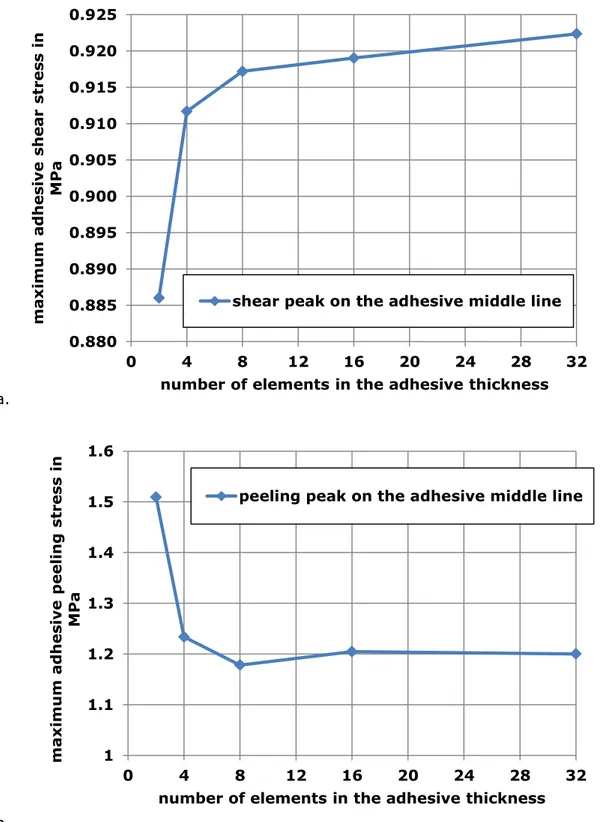
The maximum value of adhesive shear and peeling stresses depends on the mesh density. As the objective of this comparison of PS and 3D FE predictions is to assess the relevance of the 1D-beam model, the dependency of shear and peeling peaks on the mesh density has to be addressed. The study consists then in measuring the maximum values of the adhesive shear and peeling stresses as a function of the number of elements in the adhesive layer thickness. The number of elements in the adhesive layer varies, while keeping the aspect ratio of the smallest element in the adhesive layer (located at both overlap ends) equal to 1. It is shown that the shear (peeling) peak increases (decreases) with the increasing number of elements in the adhesive layer (see Fig. 13). However, this increasing or decreasing tendency significantly slows down with the increasing number of elements. Tab. 2 shows changes to the adhesive shear and peeling peaks for varying numbers of elements, relative to those for 32 elements. It can be observed that these relative differences are quite low, except for the peeling peak for the case with 2 elements. It could be thought that the hypothesis of an elastic perfectly plastic adhesive material behavior allows for the saturation of the adhesive peak stresses, contributing to low variations. In order to understand the elevated difference on the peak stress for the case with 2 elements, the shear and peeling peak adhesive stress
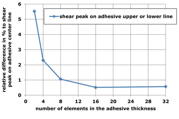
31 on the upper (or lower) external line of the adhesive layer is measured while the number of elements varies. These peaks on the adhesive upper (or lower) line are located at overlap ends, as for the adhesive middle line. As shown in Fig. 14, whereas the increase of the number of elements in the adhesive layer decreases the relative difference to the middle line on the shear peak, this relative difference increases significantly. The influence of the edge effect on the adhesive stress at the middle line seems thus to be reduced by refining the mesh in the adhesive thickness. Finally, it is considered that almost steady values for shear and adhesive peaks can be obtained, when the side height of the smallest element in the adhesive layer is inferior to 0.1 mm (i.e.: four elements in an adhesive thickness of 0.4 mm).
4.3. Comparison of results
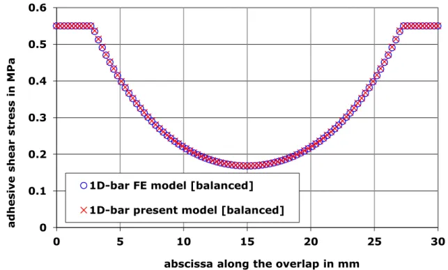
4.3.1. 1D-bar present model vs. 1D-bar FE model. Firstly, it is indicated (not presented here) that, when the adhesive is supposed linear elastic, the 1D-bar present model (without any shear in the adherends) and 1D-bar FE model provide exactly the same adhesive shear stress distribution along the overlap. Considering the elasto-plastic behavior of the adhesive, the 1D-bar present model (without any shear in the adherends) and 1D-bar FE model provide exactly the same adhesive shear stress distribution along the overlap, for the balanced and unbalanced configuration, as shown in Fig. 15 and Fig. 16, respectively.
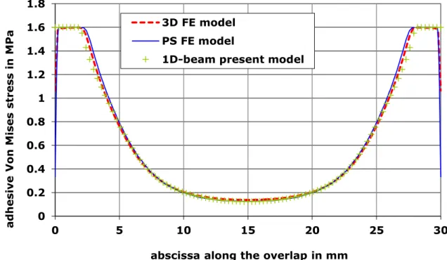
4.3.2. 1D-beam present model vs. PS and 3D FE models
. The 1D-beam present model
with a linear shear stress in the adherends is compared to the PS and 3D FE models, in case of a balanced configuration for example. The distribution of the adhesive shear, peeling and Von Mises stresses along the overlap are provided in Fig. 17, Fig. 18 and Fig. 19. Although the stress tensor component number is restricted to two in the 1D-beam present model, a good agreement is shown.32 4.3.3. Evolution of adhesive stress distribution with the applied load. In order to illustrate the effect of plasticity of the adhesive stress distribution, the adhesive shear, peeling and Von Mises stress distribution obtained with the 1D-beam present model are provided in Fig. 20, Fig. 21 and Fig. 22 respectively, at two intermediate applied loads (5 N.mm-1 and 7 N.mm-1). The structure chosen is the unbalanced configuration such that
e2=2e1=4.8 mm. The adhesive layer is meshed with four elements in its thickness
(leading to a side length of 0.1 mm for the smallest element). Furthermore, the stress distributions at an applied load of 10 N.mm-1 are compared to those predicted by the 3D
FE models, resulting in a good agreement. Moreover, it appears that the adhesive stress peak saturation is balanced by the increase of the minimal adhesive stress level reached along the overlap.
4.4. Assessment of the relevance of the model
In order to assess the relevance of the present 1D-beam model, unbalanced configurations such that e2=2e1=4.8 mm with isotropic adherends are under
consideration. The study described in this section consists of measuring the relative differences between the 3D FE model predictions and the 1D-beam model predictions, in terms of adhesive shear and peeling stresses, when: (i) the adherend stiffness varies, (ii) the adhesive thickness varies. Concerning the influence of the adherend stiffness, the variation of the adherend stiffness is achieved by fixing the Young’s modulus of the adherend 1 at its value in Tab. 1 (E1=72 GPa), while the Young’s modulus of the
adherend 2 is varying such E2=(0.5, 1, 2, 3)*E1. In the 3D FE model, the adhesive layer
is meshed with four elements in its thickness (leading to a side length of 0.1 mm for the smallest element). As shown in Tab. 3, the 1D-beam model provides adhesive shear and peeling peaks very closed to those predicted by the 3D FE model, with relative differences inferior to 10%. Moreover, in term of stress distribution along the overlap, a good correlation is obtained, as shown in Fig. 23 to Fig. 25 for the case E2/E1=3. In
particular, the overstress for abscissas close to zero, due to the unbalance of the joint, is correctly retrieved. Concerning the influence of the adhesive thickness, five adhesive