O
pen
A
rchive
T
OULOUSE
A
rchive
O
uverte (
OATAO
)
OATAO is an open access repository that collects the work of Toulouse researchers and makes it freely available over the web where possible.This is an author-deposited version published in : http://oatao.univ-toulouse.fr/ Eprints ID : 10251
To cite this version : Albagnac, Julie and Moulin, Frédéric and Eiff, Olivier and Lacaze,
Laurent and Brancher, Pierre. A three-dimensional experimental investigation of the structure of the
spanwise vortex formed by a shallow vortex dipole. (2012) In: 3rd International Symposium on
Shallow Flows - ISSF2012, 04 June 2012 - 06 June 2012 (Iowa city, United States).
Any correspondance concerning this service should be sent to the repository administrator: [email protected]
A three-dimensional experimental investigation of the structure of the
spanwise vortex formed by a shallow vortex dipole
Julie Albagnac1, Frederic Y. Moulin2, Olivier Eiff2, Laurent Lacaze2, Pierre Brancher2
1
School of Engineering, Brown University, RI, USA E-mail: [email protected]
2
Institut de Mecanique des Fluides de Toulouse, France E-mail: [email protected]
Abstract
The three-dimensional dynamics of shallow vortex dipoles is investigated by means of an innovative 3D-3C (three dimensions, three components) scanning PIV technique. In particular, the three-dimensional structure of a frontal spanwise vortex is characterized. The technique also allows the computation of the pressure field, which is not available using standard 2D PIV measurement. The influence of such complex vortex structures on the mass transport is discussed in light of the available pressure field.
1. Introduction
Most of the geophysical flows are classified into shallow flows (coastal zone) or deep stratified flows (ocean, atmosphere). A flow is qualified as shallow if the length scale of the horizontal structures is large compared to the depth of the fluid (Uijtewaal and Booij, 2000; Lin et al., 2003). In a first approximation, it is commonly assumed that the vertical confinement tends to inhibit vertical motions. Shallow flows are therefore commonly described as quasi-two-dimensional (Q2D), i.e. flows with mainly horizontal two-dimensional motions, but allowing strong vertical gradients (Jirka, 2001; Rockwell et al., 2003). This inhibition of vertical motions is also invoked to explain a self-organization into large coherent horizontal structures when an initially three-dimensional horizontal turbulent jet is generated in a shallow layer of fluid (Sous et al., 2005), evolving eventually into a large horizontal vortex dipole composed of two counter-rotating vortices in close interaction. Vortex dipoles are indeed ubiquitous coherent hydrodynamic structures in geophysical flows, motivating many studies in the past decades to investigate their dynamics, stability and transport properties.
In the context of their role as mass transport driver, Tew Kai et al. (2009) investigated the correlation between foraging trips of frigatebirds (large seabirds) over the Mozambique Channel and the Lagrangian coherent structures at the free surface. They noticed that the frigatebirds were following the contours of large vortex dipoles due to favorable fishing areas. According to Tew Kai et al. (2009), vortex dipoles, which self-propagate over large distances are associated to intense marine biological activity due to their ability to transport nutrients up to the free surface and along their trajectory. Such vertical-motion signatures of vortex dipoles in shallow flow have also been observed through the coloration of water by sediments detached from the seabed and transported to the free surface (Smith and Largier, 1995; Peregrine, 1998; Chen et al., 1999; Johnson and Pattiaratchi, 2006). These observations support the conjecture that vertical motions, thought presumably negligible due to the vertical
confinement in the framework of the Q2D approximation, could nevertheless be strong enough to play an important role in the mass transport induced by shallow water dipoles. Recently, several studies have addressed the question of this commonly assumed quasi-two-dimensionality of shallow water flows. Lin et al. (2003) and Sous et al. (2004 and 2005) observed the formation of a spanwise vortex at the front of shallow vortex dipoles resulting from decaying turbulence. Akkermans et al. (2008) performed stereoscopic PIV on electromagnetically forced shallow vortex dipoles and noticed the presence of a spanwise vortex at their front. Tentative explanations of the presence of a spanwise vortex in those two studies invoked a self-organization of the initial three-dimensional turbulence (Sous et al.) or of the vertically non-homogeneous flow field generated by electromagnetic forcing (Akkermans et al.). To identify without ambiguity the source of spanwise vortex generation, Lacaze et al. (2010) studied shallow vortex dipoles produced by a flap apparatus forcing the flow homogeneously along the whole water depth. They observed a spanwise vortex at the front, indicating that an initially two-dimensional laminar shallow dipole is also able to evolve into a three-dimensional structure. In order to investigate the conditions under which the spanwise vortex was generated, Duran-Matute et al. (2010) and Albagnac et al. (2011) realized numerical simulations and experiments, with the same experimental set-up as Lacaze et al. (2010), for a wide range of water depth and dipole propagation velocity. They showed that the existence of the spanwise vortex depends on a non-dimensional parameter taking into account both the aspect ratio (or equivalently, vertical confinement) of the flow α=h/D (where h is the water depth and D is the diameter of the dipole) and the Reynolds number associated to the horizontal propagation of the dipole Re=UD/ν (where U is the initial propagation velocity of the dipole and ν is the kinematic viscosity). When α2Re is large enough, whatever the way the shallow vortex dipole is generated, a spanwise vortex develops at the front of the vortex dipole. However, the knowledge of the complete three-dimensional structure of the vortex dipole, including the spanwise vortex, which requires access to the three components of the vorticity in a volume, has not yet been investigated, and is the objective of the present study.
The experimental set-up and the three-dimensional three components (3D-3C) Scanning Particle Image Velocimetry (SPIV) technique used for this study are described in section 2. The resulting complete three-dimensional visualization of the vortex dipole and its time evolution are shown in section 3. The time evolution of the pressure field and its derivatives in the volume, inferred from the experimental measurements obtained by the 3D-3C SPIV, are presented in section 4. Finally, a summary of the results and some perspectives of this study are given in section 5.
2. Experimental set-up
2.1 Vortex dipole generator
Vortex dipoles are generated by the closing of a pair of vertical flaps in a 2m long, 1m wide and 0.7m deep tank filled with a layer of water of depth h initially at rest (Figure 1). The flap apparatus is the same device as the one used by Billant and Chomaz (2000), Lacaze et al. (2010) and Albagnac et al. (2011), where a pair of vertical flaps, initially parallel to each
other, is put into rotation towards each other along a vertical axis. It generates two counter-rotating vortices, forming a vortex dipole, which propagates away from the flaps by mutual induction. This experimental set-up has been chosen in order to generate laminar, regular and reproducible vortex dipoles characterized by three independent experimental parameters, namely, their initial diameter D0, their initial propagating velocity U0 and the water depth h in
which they evolve. This leads to two non-dimensional numbers: the Reynolds number defined as Re=U0D0/ν (where ν is the kinematic viscosity of the water) and the aspect ratio of the
flow defined as α=h/D0. In the present study we will focus on a representative vortex dipole
with α=0.54 and Re=290 (α2Re=84.5).
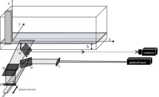
Figure 1: Experimental set-up. ”L” is a set of lenses that collimate and reduce the diameter of the laser beam and spread it into a laser sheet. ”M” indicates the mirrors. The sketch is not at scale.
In the following, x, y and z represent the streamwise, spanwise and vertical directions, respectively. The origins of the x, y and z axes are located at the initial flap trailing edge, in the vertical symmetry plane and at the tank bottom (see Figure 1). The initial time t=0s corresponds to the end of the flaps closing.
2.2 Measurement technique
In order to investigate the complete three-dimensional structure and time evolution of the vortex dipole and associated spanwise vortex, a three-dimensions, three-components scanning PIV (3D-3C SPIV) technique has been set-up. The 3D-3C SPIV technique is based on the work of Fincham (2003) and has been developed in conjunction with Boulanger at al. (2012). Briefly, the 3D-3C SPIV technique consists in reconstructing two quasi-instantaneously (i.e., regarding the flow evolution time) volumes of particles seeded in the flow and illuminated by a laser sheet (as in standard 2D PIV). On the basis of two such volumes, a three-dimensional volumetric image correlation is performed in order to obtain the three velocity components in three dimensions as well as all their spatial derivatives. The volumetric images are obtained by using a high-speed linear motor, which rapidly moves a horizontal laser sheet vertically throughout the desired depth of fluid (here the entire depth) while a high-speed camera acquires sequential and 2D-images of overlapping slices of the flow illuminated by the moving laser sheet (see Figure 1). The laser sheet is generated by a high frequency Darwin
Duo pulsed laser (Quantronix) and synchronized with the high-speed linear motor and HighSpeedStar camera (LaVision).
The first processing step is the construction of the volumetric images. The imaging of the particles in the horizontal plane is direct as the slices composing the volume are horizontal. In the vertical plane, the vertical image distribution is given by the varying intensity of the laser sheet’s Gaussian distribution and an imposed vertical overlap of the thickness of the successive illuminated slices. The Gaussian distribution of intensity in the laser sheet thickness leads to an intensity reflected by a particle depending on its vertical location in the laser sheet thickness (i.e. the more localized at the centre of the laser sheet thickness is the particle, the more intensity is reflected). Moreover, a vertical overlap in the thickness of the successive slices composing the volume yields an illumination of the same particle in successive images. A volume image of particles, or more exactly, a three-dimensional matrix of light intensity of the illuminated particles in space is obtained. A 3D correlation is then applied between the two successive volumes to obtain the three velocity components followed by a 3D spline applied to the velocity field to compute the nine components of the velocity gradient tensor. In the present study, a matrix of 60x64x32 velocity vectors is obtained to describe a physical volume of 20x20x3.5 cm3.
2.3 3D-3C SPIV: estimation of the errors and validation of the technique
Measuring a volume with a single camera induces a parallax error. To minimize this effect the camera has to be as far as possible from the field of view and the angle of aperture of the camera must be chosen as small as possible. Thus, in the present experiment the camera was located 5m away from the tank glass and the lens used is a double focus lens that has a 200 mm focal length (giving an equivalent of 400 mm focal length). In this configuration, the maximal parallax error on the whole water depth (i.e. 3.5 cm) is 60 µm.
The motion of the motor may be a source of vibration for the free surface. In order to measure the oscillations of the free surface generated by the motor motions, a Schlieren technique was employed in the two following situations: without motion of the motor and with a constant acceleration of the motor a=250 ms-2. The motion of the motor was not observed to generate measurable oscillations at the free surface.
A computer controls the motor position but there is always a discrepancy between the actual position of the laser sheet and the computer command. First, there is an absolute error: the deviation of the real position of the motor from the command position. Second, if the absolute error is not reproducible for all the scans, there is a relative error, which is the deviation of the real position of the motor for the scan of the second volume compared to the real position in the scan of the first volume of the burst. Those errors have been measured by scanning a solid transparent object containing particles and a volume of fluid at rest, and the sum of the absolute and relative error was estimated as being less than 100µm.
The error linked to the processing can be estimated through the dispersion of the displacement measured in the volume of fluid at rest. The standard deviation of the dispersion gives a processing error below 17µm for displacements.
Finally the errors associated to the 3D-3C SPIV are of the same order as the errors associated to the more classical 2D PIV (0.1 pixel) and are neglected here.
3. Time evolution of the 3D structure of a vortex dipole and its spanwise vortex
The criteria chosen here for the vortex identification is the λ2-criterion and is based on the fact
the pressure gradient is equal to zero and the second order derivatives of the pressure field must be positive in two orthogonal directions that define a plane identifying the vortex section. This condition can be examined by considering the symmetric (D) and anti-symmetric (Ω) part of the velocity gradient ▽u=D+ Ω through the symmetric tensor
G=D.DT-Ω.ΩTwith real eigenvalues
λ
1≥λ
2 ≥λ
3. The negative values of λ2 are associatedwith the presence of a vortex (Jeong and Hussain (1995)).
In the present study, the detection of the vortices is realized by operating the three following steps. First, the λ2-criterion is computed in the whole volume on a gross meshing and the n
meshes corresponding to a negative λ2 value are retained as n potential vortices. Second, the
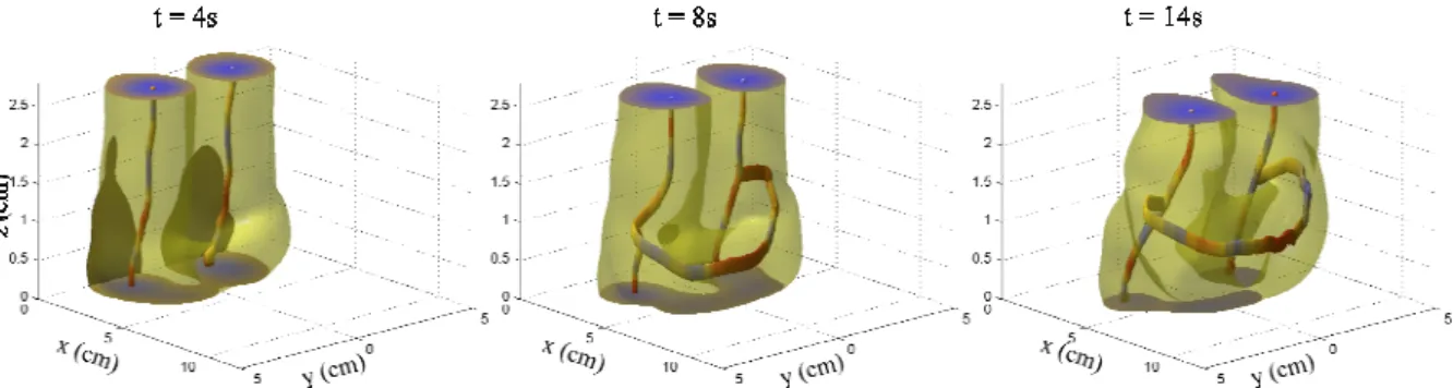
vorticity vector, which points the direction of the vortex, is considered at the n points and leads to the next mesh point belonging to the same vortex in the neighbourhood. After this step, a fair amount of the n points have been merged together into vorticity lines. Third, if two vorticity lines are close each to the other and have the same direction, then they are considered as belonging to the same vortex and are combined into a single vorticity line. In the present study, by the end of this process, two or three vortices (when the spanwise vortex is present at the front of the dipole) are generally identified: the two main vortex dipole cores and the spanwise vortex. Figure 2 displays a time evolution of the three-dimensional vorticity lines identified by this method along with iso-surfaces of the norm of vorticity.
Figure 2: Iso-surface of the norm of vorticity and vorticity lines (see text). The color along the vorticity lines indicates the local value of stretching along the line. The vortex dipole was generated with non-dimensional parameters (Re,α)=(290,0.54). Snapshots of the vortex dipole are presented at t=[4,8,14] s, respectively, from left to right.
In figure 2, only the two almost vertical coherent vortices composing the vortex dipole are present at t=4s. The vortex dipole propagating upon a solid surface develops a boundary layer due to the no-slip condition at the bottom. The vertical shear associated to the no-slip condition induces a bending of the vortices close to the bottom, as observed in figure 2.
At t=8s, the λ2-criterion detects a spanwise vortex at the front of the vortex dipole. The color
along the vorticity lines indicates that the stretching is maximal at the front of the dipole, close to the vertical plane of symmetry of the vortex dipole. This observation supports the explanation for the spanwise vortex generation proposed by Lacaze et al. (2010) who suggested that the stretching exerted by the dipole on the horizontal vorticity field of the developing boundary layer tends to focalize and amplify this vorticity, leading eventually to the formation of a coherent spanwise vortex. Between t=8s and t=14s, the spanwise vortex has moved up at the front of the primary vortex dipole. By t=8s, the spanwise vortex side branches are observed to have merged with the primary vortices composing the dipole up to the free surface. Note that the apparent orthogonal reconnection between the spanwise vortex and the primary vortices in figure 2 is not physical and is purely due to the processing.
4. Reconstructed pressure fields and its derivatives
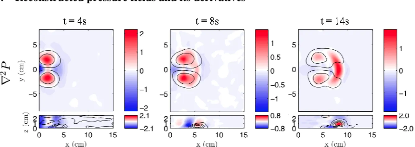
Figure 3: Slices are extracted from the 3D measurement and correspond to the horizontal plane at z=h/3 (top) and the vertical plane of symmetry of the dipole y=0 (bottom). The black contours in the horizontal slice are iso-contours of the vertical vorticity ωz (top) and iso-contours of the spanwise
vorticity ωy in the vertical plane (bottom). The color is associated to the Laplacian of the pressure. The
vortex dipole corresponds to the generation parameters (Re,α)=(290,0.54). From left to right, snapshots of the vortex dipole are presented at t=[4,8,14] s, respectively.
Figure 3 shows slices extracted from the 3D-3C SPIV measurements of a vortex dipole associated to (Re,α)=(290,0.54) at t=[4,8,14]s in the horizontal plane z=h/3 and the vertical plane of symmetry y=0. The black contours are iso-contours of the vorticity perpendicular to the plane considered (namely ωz in the horizontal plane and ωy in the vertical one). The color
is associated with the Laplacian of the pressure field. It should be recalled that a vortex can be identified by a sectional minimum of pressure, which is equivalent to a maximum of the Laplacian of the pressure.
In figures 3, according to the pressure criterion, only the primary vortices composing the vortex dipole are observed at t=4s. At t=8s, the boundary layer generated by the vortex dipole propagation upon the solid bottom has become slightly thicker. In the vertical symmetry plane, a positive Laplacian of pressure is observed in the upper part of the boundary layer and its altitude corresponds to the location of the spanwise vortex given by the λ2-criterion in
figure 2 at t=8s. At t=14s, in the vertical plane of symmetry, the black contours of the spanwise vorticity indicate a spanwise vortex detached from the boundary layer vorticity and the core of the spanwise vortex is clearly marked by a maximum of Laplacian of pressure. At this time the altitude of the spanwise vortex is approximately z=h/3. Indeed, the spanwise vortex is also detected in the horizontal plane z=h/3, at the front of the primary vortices through its signature by a local maximum of the pressure Laplacian.
The ability of the flow to put sediments into suspension can be studied through the strength of the vertical gradient of pressure. Snapshots of the time evolution of the vertical gradient of pressure are shown in figure 4.
At t=4s, in the horizontal plane, the vertical gradient of pressure is negative between the two primary vortices and positive at the front and at the rear of the vortex dipole. In the horizontal plane, along the streamwise direction, this quasi-symmetry rear-front of the vertical gradient of pressure (positive on each side) is an additional evidence of the initial quasi two-dimensionality of the vortex dipole. At t=8s, the positive vertical gradient of pressure becomes predominant at the front of the dipole. The negative vertical gradient of pressure is mainly located between the two primary vortices and slightly extends in the vertical plane of symmetry ahead of the primary vortices centroids. This feature is even more noticeable at t=14s. Moreover, the streamwise position of the negative vertical gradient of pressure is just
between the streamwise position of the primary vortices (black contours in the horizontal plane) and the streamwise position of the spanwise vortex (black contours in the vertical plane of symmetry). The likely upwelling associated to the negative vertical gradient of pressure would then take place ahead of the vortex dipole and at the rear of the spanwise vortex.
Figure 4: Slices are extracted from the 3D measurement and correspond to the horizontal plane at z=h/3 (top) and the vertical plane of symmetry of the dipole y=0 (bottom). The black contours in the horizontal slice are iso-contours of the vertical vorticity ωz (top) and iso-contours of the spanwise
vorticity ωy in the vertical plane (bottom). The color is associated to the vertical gradient of the
pressure. The vortex dipole corresponds to the generation parameters (Re,α)=(290,0.54). From left to right, snapshots of the vortex dipole are presented at t=[4,8,14] s, respectively.
The differences observed for the dipole in early quasi two-dimensional dipole state, at t=4s, and for the evolving fully three-dimensional dipole at t=14s highlights the possible role played by the spanwise vortex for particle resuspension, which has been observed for in-situ vortex dipoles as cited above. Indeed, at the front of the dipole, the spanwise vortex could swipe the sediments on the bottom back towards the primary vortices forming the dipole. Simultaneously, the dipole’s horizontal velocity field can be responsible for moving the sediments forward at the front. The combination of these two mechanisms could lead to an efficient bedload transport and suspension of bed sediment and nutrients.
5. Conclusion
In the present experimental study, a 3D-3C SPIV technique has been developed and set-up with the aim of obtaining a better understanding on the full three-dimensional structure of a shallow vortex dipole and its associated spanwise vortex. In particular, measurements in a volume of the three components of the velocity and its nine gradients, resolved in time, allows access to all the terms of the Navier Stokes equations, including the pressure field and its gradient.
The present study reveals that the stretching zone, which contributes to the generation of the spanwise vortex, reaches a maximum of intensity at the front of the dipole, in the vertical symmetry plane. This location corresponds to the zone where the spanwise vortex is observed in its premature stage (see figure 2). The side branches of the spanwise vortex starting from the vertical plane of symmetry at the front of the vortex dipole are tracked in 3D space with a vortex recognition algorithm based on the λ2-criterion and the vorticity vector. The spanwise
vortex branches are observed to incline upstream and upwards and to reconnect with the primary vortices composing the vortex dipole.
To help interpret previous in-situ observations of mass transport associated with shallow water dipoles, the pressure field and its derivatives were also computed. It is shown that the
vertical gradient of pressure is negative and exhibits a minimum at the front of the vortex dipole and at the rear of the spanwise vortex. The mass transport inferred in natural flows is therefore expected to originate from this region of the flow and to be controlled by the presence of the spanwise vortex.
Future work includes further experiments in the presence of a bed of particles at the bottom of the tank in order to qualify and quantify the effect of the vortex dipole with or without spanwise vortex (depending on the value of α2Re) on the transport of sediments.
The three dimensional experimental data will also be used as an initial condition into a numerical code to investigate the Lagrangian transport of particles.
References
Akkermans, R., Cieslik,A., Kamp, L., Clercx, H., and Van Heijst, G. (2008). The three dimensional structure of an electromagnetically generated dipolar vortex in a shallow fluid layer. Phys.Fluids, Vol. 554, 20:116601.
Albagnac, J., Lacaze, L., Brancher, P. and Eiff, O. (2011). On the existence and evolution of a spanwise vortex in laminar shallow water dipoles. Phys.Fluids, Vol. 23, 086601.
Boulanger, N., Eiff, O., Paci, A., Fincham, A. and Moulin, F.M. (2012). A novel scanning correlation imaging velocimetry (SCIV) technique applied to turbulent lee-wave breaking. To be submitted to Exp. Fluids.
Billant, P. and Chomaz, J.M. (2000). Experimental evidence for a new instability of a vertical columnar vortex pair in a strongly stratified fluid. J. Fluid Mech., Vol. 418, 167-188. Chen, Q., Dalrymple, R.A., Kirby, J.T., Kennedy, A.B. and Haller, M.C. (1999). Boussinesq
modeling of a rip current system. J. Geophys. Res., Vol. 104(C9), 20617-20637.
Duran-Matute, M., Albagnac, J., Kamp, L. and Van Heijst, G. (2010). Dynamics and structure of decaying shallow dipolar vortices. Phys.Fluids, Vol. 22, 116606.
Fincham, A. (2003). 3 component, volumetric, time-resolved scanning correlation imaging velocimetry. Proc. 5th Inter. Symp. On Particle Image Velocimetry, Busan, Korea, 2-16.
Jeong, J. and Hussain, F. (1995). On the identification of a vortex. J. Fluid Mech., Vol. 285, 69-94.
Jirka, G. (2001). Large scale flow structures and mixing processes in shallow flows. J.
Hydraulic Research, Vol. 39, 567-573.
Johnson, D. and Pattiaratchi, C. (2006). Boussinesq modeling of transient rip currents. Coast.
Eng., Vol. 53, 419-439.
Lacaze, L., Brancher, P. Eiff, O. and Labat, L. (2010). Experimental characterization of the 3D dynamics of a laminar shallow vortex dipole. Exp.Fluids, Vol. 48(2), 225-231. Lin, J., Ozgoren, M. and Rockwell, D. (2003). Space-time development of the onset of a
shallow-water vortex. J.Fluid.Mech., Vol. 485, 33-66.
Peregrine, D.H. (1998). Surf zone currents. Theoret. Comput. Fluid Dynamics, Vol. 10, 295-309.
Rockwell, D., Lin, J.C., Fu, H. and Orgozen, M. (2003). Vortex formation in shallow Flows.
Smith, J., and Largier, J. (1995). Observations of nearshore circulations: Rip currents.
J.Geophys.Res., Vol. 100, 10967-10975.
Sous, D., Bonneton, N. and Sommeria, J. (2004). Turbulent vortex dipoles in a shallow water layer. Phys.Fluids, Vol. 16(8), 2886-2898.
Sous, D., Bonneton, N. and Sommeria, J. (2005). Transition from deep to shallow water layer: formation of vortex dipoles. European Journal of Mechanics B/Fluids, Vol. 24, 19-32. Tew Kai, E., Rossi, V., Sudre, J., Weimerskirch, H., Lopez, C., Hernandez-Garcia, E.,
Marsac, F. and Garcon, V. (2009). Top marine predators track Lagrangian coherent structures. PNAS. Vol. 106(20), 8245-8250.
Uijtewaal, W,S,J., and Booij, R. (2000). Effects of shallowness on the development of free-surface mixing layers. Phys.Fluids, Vol. 12(2), 394-402.