Pépite | Développement numérique d’un macro-elément pour le calcul des pieux sous sollicitation axiales, transversales et groupe de pieux

Texte intégral

(1)Thèse de Insan Kamil, Université de Lille, 2019. Université de Lille Ecole Doctorale Science Pour l'ingénieur Laboratoire de Génie Civil et géo géo-Environnement Environnement (LCGgE). Pour l'obtention du grade de DOCTEUR DE UNIVERSITÉ DE LILLE Dicipline : Génie civil Par Insan KAMIL. Macro-Element Element Modeling For Single Pile And Pile Group (Développement Développement Numérique d’un Macro Macro-Elément Elément Pour Le Calcul des Pieux Sous Sollicitation Axiales, Transv Transversales et Groupe de Pieux) Soutenue le 10 Juillet 2019 Devant de jury composé de: Isam SHAHROUR. Professeur, Universit Université de Lille. Président. Ahmed ARAB. Professeur, Universit Université Hassiba Benbouali De Chlef. Rapporteurs. Daniel DIAS. Professeur, Universit Université Grenoble-Alpes. Rapporteurs. Sébastien BURLON Ingéénieur de Recherche, Terrasol-Setec. Examinateurs. Alia HATEM. Ingéénieur de Recherche, ARCADIS. Examinateurs. Hussein MROUEH. Professeur, Universit Université de Lille. Directeur. © 2019 Tous droits réservés.. lilliad.univ-lille.fr.

(2) Thèse de Insan Kamil, Université de Lille, 2019. ABSTRACT The proposed method presents a simple analysis of Soil-Structure Interaction (SSI) for deep foundation under static load that is applied for single pile and pile group. A model based on macro-element concept is developed to study the SSI taking into account the different nonlinearities. Its formulation is based on the theory of elastoplasticity and is inspired by European standards (Eurocodes 7 and 8). Wherein, the different parameters are defined from laboratory or in situ tests, or from numerical simulations under static conditions. This model reduces computational costs because the nonlinearities related to the SSI are concentrated in particular points of the computation model. The advantage of macroelement lies in its formulation in forces and displacements, which facilitates its use for the justification of the foundations (bearing capacity, sliding, detachment, settlements, translations, distortions and rotations). Furthermore, this macroelement is implemented in a Finite Element Method framework as a fish function in Flac3D. This tool is capable of simulating the SSI in the monotonic loaded pile. The proposed model has been validated with pile load test results, load transfer method (based on Frank and Zhao method) and computer programming (conventional Flac3D and Pilate). The approach succeeds with a good performance. Additionally, the efficiency and practical application of this method in the computation finite-element analysis are feasible for Single Pile and Pile Group . Keywords: Macro-element, Elastoplasticity, Single Pile, Pile Group, Monotonic Load, Flac3D. ii © 2019 Tous droits réservés.. lilliad.univ-lille.fr.

(3) Thèse de Insan Kamil, Université de Lille, 2019. Développement Numérique d’un Macro-Elément Pour Le Calcul des Pieux Sous Sollicitation Axiales, Transversales et Groupe de Pieux RÉSUMÉ La méthode proposée présente une analyse simple de l’interaction sol-structure (SSI) pour le calcul des pieux sous sollicitation axiales, transversales et groupe de pieux. Un modèle basé sur le concept de macroéléments est développé pour étudier la réponse du pieu en prenant en compte les différentes non-linéarités. Sa formulation est basée sur la théorie de l'élastoplasticité et s'inspire des normes européennes (Eurocodes 7 et 8). Les différents paramètres du modèle sont définis à partir d'essais en laboratoire ou in situ, ou à partir de simulations numériques dans des conditions statiques. Ce développement réduit les coûts de calcul car les non-linéarités liées à l'interaction Sol-Structure sont concentrées dans des points particuliers du modèle de calcul. L'avantage du macroélément réside dans sa formulation en forces et déplacements, ce qui facilite son utilisation pour la justification des fondations (capacité portante, glissement, détachement, tassement, translation, distorsions et rotation). De plus, ce macroélément est implémenté dans le cadre de la méthode des différences finis en tant que fish function dans Flac3D. Cet outil est capable de simuler le comportement d'un pieu sous charge monotone verticale et transversale. Le modèle proposé a été validé par les résultats des tests de chargement de pieu, des résultats numériques tels que la méthode des courbes de transfert (basée sur la méthode de Frank et Zhao) et les approches conventionnelles (Flac3D). De plus, l'efficacité et l'application pratique de cette méthode dans le calcul de groupe de pieux est aussi démontrée. mots clés: Macro-élément, élastoplasticité, pieu isolé, groupe de pieux, Charge monotone, Flac3D. iii © 2019 Tous droits réservés.. lilliad.univ-lille.fr.

(4) Thèse de Insan Kamil, Université de Lille, 2019. ACKNOWLEDGMENT I wish to deliver my special credit to my supervisor, Prof Hussein MROUEH, who gave me an opportunity working in Macro-element. My great appreciation also extends to DR Sébastien BURLON who first introduced me to the concept of macro-element and had been guiding me much in understanding and analyzing the numerical computational system. I feel lucky getting the opportunity of working under their supervision. I would like to extend my appreciation to the Director of Laboratoire de Génie Civil et géo-Environnement, Prof Isam SAHROUR, for the help and warm welcome to me. I also extend my appreciation to the reviewers, Prof. Ahmed ARAB and Prof. Daniel DIAS, for the review and suggestion in my defence. I am indebted to my late parent (may the peace upon them), my wife and my daughters who continuously support and encourage my study abroad. Also to The Ministry of Research, Technology and Higher Education of Indonesia as the founding of my research.. iv © 2019 Tous droits réservés.. lilliad.univ-lille.fr.

(5) Thèse de Insan Kamil, Université de Lille, 2019. TABLE OF CONTENT ABSTRACT. ........................................................................................................................ ii. RÉSUMÉ. ....................................................................................................................... iii. ACKNOWLEDGMENT ......................................................................................................... iv TABLE OF CONTENT ........................................................................................................... v TABLE OF FIGURE ............................................................................................................. vii LIST OF TABLE ..................................................................................................................... xi NOMENCLATURE .............................................................................................................. xiii GENERAL INTRODUCTION ............................................................................................... 1 CHAPTER I: STATE OF ART .............................................................................................. 5 I.1 REVIEW OF PILE DESIGN ........................................................................................... 6 I.2 BEHAVIOUR OF PILE UNDER MONOTONIC LOAD ................................................ 7 I.2.1 Experimental Observation of the Soil-Structure Interaction .................................... 7 I.2.2 Load Distribution On Pile Group............................................................................ 10 I.3 CONVENTIONAL PREDICTION METHODS ............................................................ 12 I.3.1 Parameters Influence............................................................................................... 12 I.3.1.1 Installation Effect ....................................................................................... 12 I.3.1.2 Time effect ................................................................................................. 13 I.3.1.3 Compressibility of Pile ............................................................................... 14 I.3.2 Loads Transfer T-z Method .................................................................................... 16 I.3.3 Loads Transfer P-y Method .................................................................................... 26 I.3.4 Hyperbolic Method ................................................................................................. 30 I.4 FINITE ELEMENT METHOD ...................................................................................... 34 I.5 MACRO-ELEMENT MODELING ................................................................................ 36 I.5.1 Macro-element Method for Shallow foundation .................................................... 37 I.5.2 Macro-element Method for deep foundation .......................................................... 41 I.6 RESULT ......................................................................................................................... 41 CHAPTER II: DEVELOPMENT OF MACRO-ELEMENT ............................................ 46 II.1 CONCEPT OF MACRO-ELEMENT ............................................................................ 48 II.2 THE ELASTOPLASTIC LOAD-DISPLACEMENT LAW ......................................... 49 v © 2019 Tous droits réservés.. lilliad.univ-lille.fr.

(6) Thèse de Insan Kamil, Université de Lille, 2019. II.2.1 Relative Displacements in Elastic Response ........................................................ 51 II.2.2 Relative Displacements in Elastic Perfectly-Plastic .............................................. 55 II.2.3 Elastoplasticity With Hardening Law ................................................................... 57 II.2.4 Relative Displacement in Plastic Potential and Flow Rule ................................... 58 II.3 SYNTHESIS OF ELASTOPLASIC MACRO-ELEMENT PARAMETERS ............... 59 II.3.1 Vertical load .......................................................................................................... 60 II.3.2 Transversal load..................................................................................................... 60 II.4 COMPARISON TO CONVENTIONAL LOAD TRANSFER METHOD ................... 61 II.4.1 Case Studies For Vertical Load Response ............................................................ 61 II.4.2 Case Studies For Transversal Load Response ....................................................... 67 II.5 RESULT ........................................................................................................................ 71 CHAPTER III: APPLICATION AND VALIDATION OF MACRO-ELEMENT ......... 72 III.1 SINGLE PILE ............................................................................................................... 73 III.1.1 Vertically Loaded Pile ......................................................................................... 73 III.1.2 Transversally Loaded Pile .................................................................................... 76 III.2 PILE GROUP ............................................................................................................... 78 CONCLUSION AND PERSPECTIVE ................................................................................ 86 BIBLIOGRAPHY................................................................................................................... 88. vi © 2019 Tous droits réservés.. lilliad.univ-lille.fr.

(7) Thèse de Insan Kamil, Université de Lille, 2019. TABLE OF FIGURE Figure I.1. Piles capacity mechanism (a) axial loads (b) lateral load ......................................... 7 Figure I.2. Bi-directional loading test ......................................................................................... 8 Figure I.3. Loads-Displacement curve, pile is loaded until Ultimate state ................................ 8 Figure I.4. Loads transfer curve (shaft and tip) .......................................................................... 9 Figure I.5. Lateral load test layout ............................................................................................ 10 Figure I.6. Lateral load test layout ............................................................................................ 10 Figure I.7. Load settlement response of the piles at different location of nine-pile group connected to rigid pile-cap (Zhang et al, 2013) ........................................... 11 Figure I.8. (a)Soil layer deformation on Displacement pile on driving pile (b) NonDisplacement on bore pile ............................................................................ 12 Figure I.9. Variation of pile-capacity with time (Fleming et al, 2009) .................................... 14 Figure I.10. The progressive failure of along pile .................................................................... 15 Figure I.11. Variation of reduction factor with pile stiffness ratio ........................................... 16 Figure I.12. The mechanism on axially monotonic load (a) transfer mechanism and (b) spring-mass model ....................................................................................... 16 Figure I.13. End bearing resistance considering (a) plugged condition and (b) unplugged condition ....................................................................................................... 17 Figure I.14. Free body diagram of pile segment....................................................................... 18 Figure I.15. Example of Pressure-meter Test result ................................................................. 19 Figure I.16. (a) Load-Transfer mechanism (b) the T-z curve (c) the q-z curve (after Frank and Zhao,1982) ............................................................................................ 20 Figure I.17. Model of the full pile (a) model of the base of pile (b) ........................................ 21 Figure I.18. Value of kp and Def/B............................................................................................ 22 Figure I.19. Friction curve fsoil(pl*) .......................................................................................... 23 Figure I.20. Area A and perimeter P to be used for open-end steel piles & sheet piles ........... 25 Figure I.21. Unit stress distribution in lateral load ................................................................... 26 Figure I.22. Behavior of P-y curve (Coduto,1994)................................................................... 26 Figure I.23. Pile segment discretization pile element and soil element. .................................. 27 Figure I.24. The P-y curve at pile segment adjusts with depth ................................................ 28 Figure I.25. Soil reaction against lateral displacement (after Frank, 1999) ............................ 30 Figure I.26. Hyperbolic representation of stress-strain, Kondner (1963) (a) real curve (b) transformed curve......................................................................................... 31 Figure I.27. Observed and theoretical relationship between shaft resistance and displacement (Zhang et al. 2013) ................................................................. 31 vii © 2019 Tous droits réservés.. lilliad.univ-lille.fr.

(8) Thèse de Insan Kamil, Université de Lille, 2019. Figure I.28. Observed and theoretical relationship between end-bearing resistance and displacement ( Zhang et al. 2013) ................................................................ 32 Figure I.29. Schematic shape of the P-Y curve (Bouafia A, 2013) .......................................... 32 Figure I.30. Pile segment discretization into pile element and soil element. ........................... 34 Figure I.31. The pattern of Plasticity Flow indicator on Flac3D.............................................. 36 Figure I.32. General structure of macro-element a. Structure of macro-element b. System analogy ......................................................................................................... 37 Figure I.33. Evolution of the charge surface within the rupture criterion of the Crémer model (Grange, 2008) .................................................................................. 38 Figure I.34. General structure of macro-element of Chatzigogos,2007. .................................. 38 Figure I.35. Ultimate and yield surface by Chatzigogos,2007. ............................................... 39 Figure I.36. Lay out of variable global studied a. efforts b. displacement (Grange, 2008) ..... 39 Figure I.37. Single Macro-element model (Abboud et all, 2017)............................................. 40 Figure I.38. Distributed Macro-element model (Abboud et all, 2017) ..................................... 40 Figure I.39. Hybrid Macro-element model (Abboud et al, 2017)............................................. 40 Figure I.40. (a) Macro-element on lateral load, (b) components of macro-element (Taciroglu, 2006) ......................................................................................... 42 Figure I.41. (a) Macro-element on multi axial load (b) basic element on multi axial model (Rha and Taciroglu, 2007) ........................................................................... 43 Figure I.42. Determining The initial stiffness parameter of the hypolplastic macro-element (Zheng li, 2015) ............................................................................................ 44 Figure I.43. Failure envelope in the H:M/D loading plane: fitting curve based on model tests data and numerical simulation (Zhuang Ji, 2019)............................... 45 Figure I.44. Failure surface in 3D H-M-V space (Zhuang Ji, 2019) ........................................ 45 Figure II.1. The concept of Macro-element that work on single macro element. ................... 48 Figure II.2. The concept of Macro-element that is attached on Flac3D for the single pile ...... 49 Figure II.3. The concept of Macro-element that is attached on Flac3D for the Group pile ..... 49 Figure II.4. Elastic and plastic zone in the stress-strain curve ............................................... 50 Figure II.5. Elastic and plastic zone in the stress-strain curve ............................................... 51 Figure II.6. Model of macro-element at a mass ....................................................................... 52 Figure II.7. (a) Sketch of mesh and boundary condition, (b) Model in Flac3D ....................... 54 Figure II.9. Elastic-perfectly plastic zone in the stress-strain curve...................................... 55 Figure II.10. The stress-displacement curve on Elastic-perfectly plastic state. ..................... 56 Figure II.11. Real Hyperbolic graphic ...................................................................................... 57 Figure II.12. Influence of coefficient b to the curve ................................................................. 58 viii © 2019 Tous droits réservés.. lilliad.univ-lille.fr.

(9) Thèse de Insan Kamil, Université de Lille, 2019. Figure II.13. The iterative development procedure of the mathematical tool plastichardening zone in the stress-strain curve .................................................... 58 Figure II.14. (a) The single Macro-element for single pile and (b) Macro-element on Flac3D for pile group on vertically load ...................................................... 61 Figure II.15. (a) Sketch of mesh and boundary condition on the single Macro-element for single pile and (b) Model for Macro-element on Flac3D ............................ 62 Figure II.16. The load-settlement curve at the pile head of single pile from soil type 1 from 10m depth ( D= 30 cm to D= 60cm) ............................................................ 64 Figure II.17. The load-settlement curve at the pile head of single pile from soil type 1 from 10m depth ( D= 70 cm to D= 100cm). ......................................................... 64 Figure II.18. The load-settlement curve at the pile head of single pile from soil type 2 from 20m depth ( D= 30 cm to D= 60cm). ........................................................... 65 Figure II.19. The load-settlement curve at the pile head of single pile from soil type 2 and 20m depth ( D= 70 cm to D= 100cm). ......................................................... 65 Figure II.20. The comparison curve between T-z method and the macro-element method due to the variation of slope coefficient on macro-element Cs (20m depth and diameter 70 cm ) .................................................................................... 66 Figure II.22. (a) Mesh and boundary condition (b) The plasticity flow on Flac3D in macroelement method (c) The plasticity flow on Conventional Flac3D. .............. 67 Figure II.23. (a) The single Macro-element for single pile and (b) Macro-element on Flac3D for pile group on Lateral load .......................................................... 67 Figure II.24. The load-settlement curve for at the pile head of single pile from Homogenous soil with 10m depth ( D= 30 cm to D= 100cm). .................... 69 Figure II.25. The load-settlement curve for at the pile head of single pile from bi-layered soil with 10m depth ( D= 30 cm to D= 100cm). .......................................... 70 Figure III.1. Sketch of Flac3D mesh and boundary condition, (a) Conventional method (b) Macro-element method ................................................................................ 74 Figure III.2. (a) Model of the pile on flac3D (b) Displacement magnitude (c) Plasticity flow of soil ................................................................................................... 74 Figure III.3. (a) The simple model of the pile on flac3D for macro-element (b) Displacement magnitude .............................................................................. 75 Figure III.4 Plasticity flow of soil on Flac3D for Macro-element method in MohrCoulomb criterion. ....................................................................................... 76 Figure III.5 Measured and calculated load-settlement curve at the pile head of single pile ... 76 Figure III.6. (a) Sketch of mesh and boundary condition on the single Macro-element for single pile and (b) Model for Macro-element on Flac3d ............................. 77 Figure III.7. Comparison of predicted and measured deflection .............................................. 78. ix © 2019 Tous droits réservés.. lilliad.univ-lille.fr.

(10) Thèse de Insan Kamil, Université de Lille, 2019. Figure III.8 Calculation Value of limiting unit skin friction of soil at each segment (Zhang et al. (2013)) and the assumtion value of Em (Menard modulus) ................ 79 Figure III.9. The configuration of Four-pile group ................................................................. 80 Figure III.10 Measured and calculated load-settlement curve at the pile head of Four- pile group ............................................................................................................ 80 Figure III.11 The configuration of nine-pile ........................................................................... 81 Figure III.12 Sketch of Flac3D mesh and boundary condition (a) with pile-cap and (b) without pile-cap ............................................................................................ 81 Figure III.13. (a) model (b) plasticity flow ............................................................................... 82 Figure III.14. Load-settlement response of pile at different location of Macro-element result and Zhang et al result. ........................................................................ 83 Figure III.15. Measured and calculated load-settlement curve at the rigid pile head of ninepile group ..................................................................................................... 84 Figure III.16. Load distribution vs -settlement response of pile group .................................... 84. x © 2019 Tous droits réservés.. lilliad.univ-lille.fr.

(11) Thèse de Insan Kamil, Université de Lille, 2019. LIST OF TABLE Table I.1. Theoretical and measured load distribution tests of Koizumi and Ito (1967) .......... 11 Table I.2. Spring values simulating pile under vertical loading (Comoros et al.,2009)........... 11 Table I.3. Classification of piles (AFNOR,2012) ..................................................................... 13 Table I.4. Value for the tip bearing resistance factor kp,max for Def  5 (Burlon et al, 2014) .... 22 Table I.5. Selecting the Qi line to obtain the limit unit skin friction value qs (Burlon et al,2014) ........................................................................................................ 23 Table I.6. Value of installation factor soil-pile (Burlon et al,2014 ) ......................................... 24 Table I.7. The maximum Value ultimate skin friction qs-max .................................................... 25 Table I.8. Value of the coefficient a,b,c,n and m for PMT (Bouafia A. 2013) ......................... 33 Table I.9. Value of the coefficient a,b,n and m for Cone penetration test (Bouafia A. 2017) .. 33 Table I.10. Parameter of Macro-element (Abboud, 2017) ........................................................ 41 Table II.1. The analytic calculation of internal forces on elastic state ..................................... 53 Table II.3. Calculation on Flac3D with embedded Macro-element on elastic state ................. 54 Table II.4. Parameters of elastoplastic macro-element model.................................................. 60 Table II.4. (a) Menard Pressure-meter test for type soil 1 (layered soil) and (b) type soil 2 (Homogeneous soil) ..................................................................................... 62 Table II.5. The ultimate capacity of the pile head in each dimension of the pile in 10 m depth and soil type 1.a. ................................................................................. 63 Table II.6. The ultimate capacity of the pile head in each dimension of the pile in 20 m depth and soil type 1.b. ................................................................................ 63 Table II.7. Calculation results of the macro-element parameters at each dimension of the pile in 10 m depth and soil type 1.a. ............................................................ 63 Table II.8. Calculation results of the macro-element parameters at each dimension of the pile in 10 m depth and soil type 1.b. ............................................................ 63 Table II.9. Menard Pressure-meter test for Homogenous soil .................................................. 68 Table II.10. Calculation results of the macro-element parameters for laterally load at each dimension of the pile in 10 m depth in homogeneous soil. .......................... 68 Table II.11. Menard Pressure-meter test for Bi-layered soil .................................................... 69 Table II.12. Calculation results of the macro-element parameters for laterally load at each dimension of the pile in 10 m depth in bi-layered soil. ................................ 70 Table III.1 Soil parameter value from Pressuremetter test. ...................................................... 73 Table III. 2 Material properties ................................................................................................ 74 Table. III. 3 Macro-element parameters ................................................................................... 75 xi © 2019 Tous droits réservés.. lilliad.univ-lille.fr.

(12) Thèse de Insan Kamil, Université de Lille, 2019. Table III.4. The macro-element parameters ............................................................................ 77 Table III.5 Macro-element Parameters ..................................................................................... 79 Table III.6 Predicted pile head load for four pile-group connected by rigid pile-cap. ............. 80 Table III.7. Predicted pile head load at different location connected by rigid pile-cap ........... 82 Table III.8. Predicted pile head load at different location connected by Rigid pile-cap (Zhang et al, 2013). ...................................................................................... 83 Table III.9. Predicted pile head load by Macro-element at different location connected by flexible pile-cap. ........................................................................................... 85. xii © 2019 Tous droits réservés.. lilliad.univ-lille.fr.

(13) Thèse de Insan Kamil, Université de Lille, 2019. NOMENCLATURE Pile Properties (m2) 𝐴 B (m) C (m) Ep (GPa) hi (GPa) K L (m) Pi (m) (kN) 𝑅𝑐 (kN) 𝑅𝑠 (kN) 𝑅𝑏 (kN) 𝑄 (m) 𝑤 uz (mm) Soil Properties Em (MPa) Plm (MPa) Ple* (MPa) Es (MPa) (o)  cu (kPa) (kPa)  (kPa) . . Cross-section area of pile Diameter of pile circumference of pile at depth z Modulus young of pile Length at segment i ratio of flexibility lengh of pile Perimeter of pile at segment i Pile capacity Shaft resistance Bearing capacity internal pile force at depth z Relative movement from peak to resedual Displacement of pile segment at depth z Menard Pressuremeter modulus Limit pressure in Pressuremeter Net Equivalent Menard Limit pressure Modulus young of soil Friction angle Cohesion Undrained Stress Shear stress Poisson's ratio. Interface properties Unit end-bearing resistance (kPa) 𝑞 Unit skin resistance at section i (kPa) 𝑞 Stress (MPa)  Strain %  u mm Displacement Involved parameters of pile (kPa/mm) functions of the pressuremeter modulus Em for skin resistance 𝑘 (kPa/mm) functions of the pressuremeter modulus Em for base resistance 𝑘 (kPa) bearing capacity qb (kPa) shaft resistances qs Macroelement Properties Empirical coefficient on macroelement a (kN) Empirical coefficient on macroelement b (mm) Effective depth on macro-element Dem (m) kv (kN/mm) Slope in elastic state on macro-element for vertically loaded kh (kN/mm) Slope in elastic state on macro-element for laterally loaded Yield fy (kN) du (mm) Relative displacemen on macro-element Multiplier  Coefficient of curvature on macro-element  Slope coefficient on macro-element Cs. xiii © 2019 Tous droits réservés.. lilliad.univ-lille.fr.

(14) Thèse de Insan Kamil, Université de Lille, 2019. GENERAL INTRODUCTION. GENERAL INTRODUCTION In recent decades, a growing number of civil engineering structures have emerged in increasingly complex configurations. The complexities arise either from (i) the geometrical configuration of the structure, or (ii) the nature of the soils in which they are built, or (iii) the types of external loading, or any combination therof. The analysis and the design of these structures is not an easy task, because it requires a good knowledge of the materials under consideration, of their reaction induced by complex loadings, but also and especially a good knowledge of the boundaries conditions of the structure, in particular, the interface between the place where these solicitations originate and the structure itself. This requires a specific study which is commonly called SoilStructures Analysis. Indeed, the term “interaction” has an important meaning, since it highlights the fact that not only does the nature of the soil have an influence on the behavior of the structure, but also the structure has an influence on the behavior of the soil. There are several theories used to analyse soil-structure interaction problems. Among them, the numerical modelling, using finite element method and load transfer method (hyperstatic reaction methods), is the most suitable method because of its capability to solve the problem by taking into account the above several complexities. In practical engineering, the load transfer method is commonly used in design purpose. There is much particular interpretation to define the parameter used in this method such as pile material, type of soil, installation method and compressibility of the pile where it is provided in many codes such as API (American Petroleum Institut), Eurocode 7 and 8, AFNOR, etc. The Finite Element Method is used in the soil-structure interaction (SSI) analysis where it is possible to define more complex interactions at the local level in detail for all elements (soil, foundation, structure, etc.). However, it requires high cost in. 1 © 2019 Tous droits réservés.. lilliad.univ-lille.fr.

(15) Thèse de Insan Kamil, Université de Lille, 2019. GENERAL INTRODUCTION calculation time, complexity in mesh construction and also difficulty in post-processing result due to the complexity of the soil-structure interaction (SSI) problems involved with. Although, many computation programmings have been introduced as an effort to minimise the calculation time such as Fast Lagrange Analysis of Continua (Flac3D). However, the conventional computer programming, in rendering process of plasticity flow indicator, takes extra time in every calculation step. The plasticity flow indicator indicates that the programme did analysis and calculation to all of the constructed models to define the result. In other words, the development of a new model which gives increased efficiency, accuracy and rapid prediction is still necessary. To fill these lacks, the development of a tool that allows producing a simplified method to find out the behaviour of deep foundation embedded in the semi-infinite soil mass. The operation law will be constructed in an intermediate scale between global and local. This tool has been known as Macro-element that was initialized by Nova and Montrasio, 1991 in geotechnical engineering. The concept of this method has been introduced in the context of the shallow foundation. The evolution of macro-element into several SSI problem solving was continued by Pelluci, 1997, Cremer, 2001, Chatzigogos et al. 2007, Grange et al., 2008, Abboud et al. 2017. Afterwards, the soulution for deep foundation has been presented by Tachiroglu 2006, Rha 2007, Li 2015 and Zheng Ji, 20019. However, the developed macro-element concepts for deep foundation have been proposed only for a single pile. This thesis presents the development of macro-element model for group pile. A model based on the macroelement concept is developed to study the soil-structure interaction (SSI) taking into account the different nonlinearities. Its formulation is based on the theory of elastoplasticity and is inspired by European standards (Eurocodes 7 and 8). The parameters are defined from laboratory or in situ tests, or from numerical simulations. 2 © 2019 Tous droits réservés.. lilliad.univ-lille.fr.

(16) Thèse de Insan Kamil, Université de Lille, 2019. GENERAL INTRODUCTION under static and dynamic conditions. The computational costs are reduced because the nonlinearities related to the soil-structure interaction are concentrated in particular points of the computation model. The advantage of the macroelement lies in its formulation in forces and displacements, which facilitates its use for the justification of the foundations (bearing capacity, sliding, detachment, settlements, translations, distortions and rotations). As a result, the efficiency of the calculation will effect to both the user and the machine. The advantages at the user side are simplifying of preparation time in mesh construction, data input, and analysis result where will effect to the machine in computation time. In order to achieve the objective of this research, this study is divided into two main part. The first part is about constructing a mathematical model. And the second part deal with the running program by embedded macro-element model on Flac3d. The comparison and validation result with other approaches and field tests will be investigated to verify the accuracy and efficiency of the proposed macroelement method. This report is composed into three chapters started with bibliography synthesis. The first chapter is dealing with the synthesis of bibliography to present state of the art relating to the behaviour of the pile under monotonic axial and transversal load. Also, the parameters which influence the soil structure interaction such as installation methods, materials of the pile, and type of soil in conventional prediction method. Furthermore, It presents the constitutive law on soil structure interaction from elastic model to plastic model addressing to develop the macro-element method. The calculation method dealing with the mobilisation law of Frank and Zhao method. The previous studies about macroelement, shallow and deep foundation, are also synthesized in this chapter. The second chapter is dealing with the development of macro-element. Base on the constitutive law of soil structure interaction the governing equation for the macro-element is constructed. It is started from the elastic model to plastic model. The first step is in the elastic model, where macro-element is developed in the elastic-perfectly plastic model to 3 © 2019 Tous droits réservés.. lilliad.univ-lille.fr.

(17) Thèse de Insan Kamil, Université de Lille, 2019. GENERAL INTRODUCTION the Mohr-Coulomb plastic model dealing with the calculation result of the macro-element model. Then, It is embedded to flac3d in the elastic model, elastic-perfectly plastic and the plasticity model on the axial and transversal monotonic load on macro-element. Also, the comparison and validation result with load transfer method base on Frank and Zhao method and also using the Pilate computer programme. The third chapter is the implementation and validation. It is implemented in framework of Finite Element Method (Flac3D). Then, the result is validated with load transfer method (base on Frank and Zhao method) and computer programming (conventional Flac3D and Pilate). Next, it is compared to the other methods results, and pile load test results. Group of pile. 4 © 2019 Tous droits réservés.. lilliad.univ-lille.fr.

(18) Thèse de Insan Kamil, Université de Lille, 2019. CHAPTER I: STATE OF ART. CHAPTER I: STATE OF ART This chapter presents the behaviour of pile under monotonic axial and transversal load followed by the parameters which influence the soil-structure interactions. Then, It continues to the concept of the load transfer method (dealing with the mobilisation law of Frank and Zhao) and Finite Element Method. The constitutive laws of soil structure interaction, from elastic to plastic model, are addressed to develop the macro-element method. Furthermore, the previous studies of macroelement method, used in the shallow and deep foundation, are synthesised.. 5 © 2019 Tous droits réservés.. lilliad.univ-lille.fr.

(19) Thèse de Insan Kamil, Université de Lille, 2019. CHAPTER I: STATE OF ART I.1 REVIEW OF PILE DESIGN Piles foundation has been used in construction since prehistoric as a method of overcoming the difficulties of founding the construction on soft soil, but the design was based on experience entirely until the last of the nineteenth century. From the experimental observation of foundation, the interaction between soil and structure or known as soil-structure interaction theory can be comprehended. Also, behaviour of pile foundation while the load acting on the pile can be predicted. Some calculation methods have been proposed due to these comprehensions to predict the load-displacement analysis. The loads that are transmitted from the upper structure determining the movement of the pile. Then the interaction between pile and soil, and also pile to another pile (in case of piles group) occurs. The embedded piles reinforce and increase load capacity of soil which is the same way as the steel reinforcement in concrete. For the vertical load, the failure of pile foundation occurs at the interface between sides of the pile and soil, and at the pile base. The total shear stress at the shaft-soil interface and the base of pile achieves a limit value which is varying with depth and soil type. For the horizontal failure is resulted from lateral load or moment, the normal stress at the interface achieves a limit value which is varying with depth. The possibility of understanding the behaviour of piles are several methods proposed to analyze the complexity that exist in soil-structure interaction of pile foundation under monotonic axial and lateral load. Nowadays, there are many kinds of literature have been proposed as an approach formula for the capacity of the pile. The result of field experiences and empirical data of the piles performance have been published. Numbers of theories used to analyse the interaction between pile and soil due to the balancing approach between empirical experiences and theory. It is common progress in foundation engineering. Among them, the numerical modelling, using finite element method and load transfer method (hyperstatic reaction methods), is the most suitable method because of its capability to solve the problem by taking into account the above several complexities. In practical engineering, the load transfer method is commonly used in design purpose. Initially, It proposed by Coyle and Reese, 1966. In the construction of load transfer method, there are many proposed mobilisation theory from frank and Zhao method, hyperbolic, etc. However, most methodologies are still not applicable to routine calculation. There is much particular interpretation to define the parameter used in this method such as pile material, type of soil, installation method and compressibility of the pile where it is provided in many codes. 6 © 2019 Tous droits réservés.. lilliad.univ-lille.fr.

(20) Thèse de Insan Kamil, Université de Lille, 2019. CHAPTER I: STATE OF ART such as API (American Petroleum Institut), Eurocode 7 and 8, AFNOR, etc. The loaddisplacement response is the result of this method. The Finite Element Method is used in SSI analysis where it is possible to define more complex interactions at the local level in detail for all elements (soil, foundation, structure, etc.). However, it requires high cost in calculation time, complexity in mesh construction and also difficulty in post-processing result due to the complexity of SSI problems involved with. I.2 BEHAVIOUR OF PILE UNDER MONOTONIC LOAD The prediction of displacement-stress or displacement-load on the pile is influenced by many parameters of soil and type of pile. From experimental observation, the pattern of soilstructure behaviour can be shown by a stress-displacement curve as a simple way to understand the performance of pile. The governing equation of settlement prediction in an elastic state or a plastic state in many models that proposed by many researchers is very important as the constitutive law of calculation method in the stress-displacement prediction. I.2.1 Experimental Observation of the Soil-Structure Interaction Many studies carried out on pile load testing, most of them focused on the relationship of soil reaction and axial/lateral pile displacement. The relationship knows as the T-z curve for axial loading and P-y curve for lateral loading. Figure I.1 describes the soil-structure reaction for axial loading (Figure I.1.a) and reaction for lateral loading (Figure I.1.b). Where shaft friction and end-bearing reaction work on axial loading mechanism. The lateral reaction of soil dealing with depth works on lateral loading mechanism.. (a). (b). Figure I.1. Piles capacity mechanism (a) axial loads (b) lateral load. 7 © 2019 Tous droits réservés.. lilliad.univ-lille.fr.

(21) Thèse de Insan Kamil, Université de Lille, 2019. CHAPTER I: STATE OF ART In the practical test, the pile can be instrumented to define normal stress along the pile and obtain the result for each depth. Bi-directional loading test, introduced by Osterberg in 1986s (Osterberg,1989), is one of loading test method (Figure I.2).. Figure I.2. Bi-directional loading test This test loads the pile in compression from the bottom of pile. As the cell in the bottom expands, the end bearing Q provides reaction for the side shear F bi-directional static loading tests calculating the pile head settlements by the side shear load-displacement curve. It is obtained from the upward movement of the top of the load cell. The downward movement of the bottom of the load cell obtains the end bearing load-displacement curve.. Figure I.3. Loads-Displacement curve, pile is loaded until Ultimate state In axial static load tests (Figure I.3) is an illustration while the load applied on pile effecting to the displacement of the pile until the pile-capacity reached (Rc) and the peak resistance for bearing capacity of pile assuming 10% Diameter of the pile (API,1993). Those relationship is described by equation I.1 to I.3. 8 © 2019 Tous droits réservés.. lilliad.univ-lille.fr.

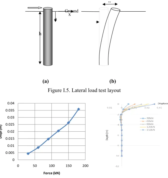
(22) Thèse de Insan Kamil, Université de Lille, 2019. CHAPTER I: STATE OF ART 𝑅𝑐 = 𝑅𝑠 + 𝑅𝑏. (I.1). 𝑅𝑠 = ∑ 𝑞 ℎ 𝑃. (I.2). 𝑅𝑏 = 𝑞 𝐴. (I.3). The experimental observation shows the contribution of shaft friction and end bearing of the pile to the force that is applied on pile. Figure I.4 illustrates the contribution of the pilecapacity between shaft resistance (Rs) and bearing capacity (Rb). The result of the T-z method is assumed as experimental test showing that the normal stress decreases with the depth. The reduction of normal stress along the pile due to the mobilised friction on the interface is very influenced to pile-capacity. When the applied load on pile reaches the top of pile-capacity (Rc), then the difference between Ultimate pile-capacity and bearing capacity is shaft friction (equation I.1). Bearing capacity (Rb) is calculated according to equation I.2, where Ab is cross-section area of the pile at base and qb is a unit end-bearing resistance. And shaft resistance (Rs) is calculated according to equation I.3, where Pi, qs and hi are the perimeter of the pile at i section, unit skin resistance and thickness of the section.. Figure I.4. Loads transfer curve (shaft and tip) The full-scale lateral load test performed to develop a load-displacement relationship. The horizontal movement occurs in field test cause of lateral load. Its relationship is recorded between lateral load dealing with depth z. During a load test, the lateral load act on the head of pile then displacement occur dealing with dept (Figure I.5.a). The displacement of the pile can be measured (Figure I.5.b). The slope of pile dealing with depth data is recorded. The load-displacement graphic that result of the field test is described in Figure I.6. Increasing of load will influence the increase of displacement. 9 © 2019 Tous droits réservés.. lilliad.univ-lille.fr.

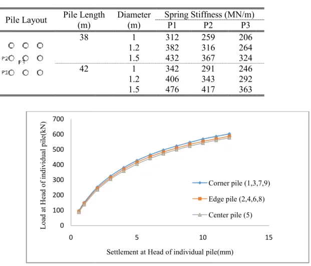
(23) Thèse de Insan Kamil, Université de Lille, 2019. CHAPTER I: STATE OF ART u Ground. z. x. h. (a). (b). Figure I.5. Lateral load test layout 0.04 0.035. Displ (m). 0.03 0.025 0.02 0.015 0.01 0.005 0 0. 50. 100. 150. 200. Force (kN). Figure I.6. Lateral load test layout I.2.2 Load Distribution On Pile Group It has been known that the load, for the stiff pile-caps, is highest at the corners then edges. But for the flexible pile-caps, the load is distributed more evenly but often at the cost of higher settlements at the centre caused by a dishing effect of the pile-cap (Rose, 2012). Whitaker (1957) reported that at the large of loading, the corner piles take the largest and the centre of the pile takes the smallest proportion. Cook (1974) also demonstrated the interaction between pile in a group. In 25-piles square group at the corner found carrying five times as much as the centre pile load. Poulos (1980) reported the load distribution test between theoretical and test result which is tested by Koizumi and Ito (1967) in 3x3 pile group (Table I.1). Comoros et al (2009) gave the summarise result of simulation by 3D non-linear analysis providing the precise response of characteristic of the pile in a group (Table. I.2). Zhang et al ( 2013) also reported the load distribution on 3x3 pile group at the center, edges and mid-edges 10 © 2019 Tous droits réservés.. lilliad.univ-lille.fr.

(24) Thèse de Insan Kamil, Université de Lille, 2019. CHAPTER TER I: STATE OF ART (Figure.I.7) where the largest is at corner , the second largest at edge and the smallest at the center. The stiff pile-cap would transfer the loads from the central piles and redistribu redistribute them to the outer piles, piles at the edge take up a higher fraction of the total loads and are subject to higher axial and bending loads loads. For large pile groups, the axial loads on piles with a flexible raft are relatively uniform distributed; however, with a rigid raft, the corner piles carry loads significantly higher than the centre piles (Chow H and Poulos HG, 2015). 2015) Table I.1.. Theoretical and measured load distribution tests of Koizumi and Ito (1967) Pile Location Center Mid-side Corner. Pile Load/Average Pile Load Theoretical Measured 0.35 0.46 0.82 0.86 1.35 1.2. Table I.2. Spring values lues simulating pile under vertical loading ((Comoros Comoros et al.,2009) al.,2009 Pile Layout. Pile Length (m) 38. Load at Head of individual pile(kN). 42. Diameter (m) 1 1.2 1.5 1 1.2 1.5. Spring Stiffness (MN/m) P1 P2 P3 312 259 206 382 316 264 432 367 324 342 291 246 406 343 292 476 417 363. 700 600 500 400 300. Corner pile (1,3,7,9). 200. Edge pile (2,4,6,8). 100. Center pile (5). 0 0. 5. 10. 15. Settlement at Head of individual pile(mm). Figure I.7.. Load settlement response of the piles at different location of nine nine-pile group connected to rigid pile pile-cap (Zhang et al, 2013). 11 © 2019 Tous droits réservés.. lilliad.univ-lille.fr.

(25) Thèse de Insan Kamil, Université de Lille, 2019. CHAPTER I: STATE OF ART I.3 CONVENTIONAL PREDICTION METHODS The popular prediction methods to account the soil-structure interaction for the pile foundation are the T-z method for vertical displacement, the P-y method for lateral displacement, the hyperbolic method as a more simple calculation until Finite Element method as the latest method that bases of the computer programming calculation. I.3.1 Parameters Influence In addition to soil properties, the behaviour of pile foundation essentially also depends on the installation method, the pile material and the compressibility. I.3.1.1 Installations Effect Three installations technique of piles are mentioned due to the displacement of soil during installation. The first technique of installation, relatively effecting big displacement on soil, is the large displacement pile such as wooden pile, spun pile, and driven steel closed end pile etc. The second technique, relatively effecting less displacement on soil than, is the small displacement such as micropile (Figure I.8.a). Then non-displacement pile is the third installation technique by boring such as bore pile etc (Figure I.8.b).. Q Pile Initial layers Sheared soil layer layers. Bored Hole. Qtip (b). (a). Figure I.8. (a)Soil layer deformation on Displacement pile on driving pile (b) NonDisplacement on bore pile But, The standard NF P 94-262 (AFNOR, 2012) proposes two installation technique of piles as displacement pile and non-displacement pile followed by 20 type number of the pile which is divided into 8 group code (table I.3).. 12 © 2019 Tous droits réservés.. lilliad.univ-lille.fr.

(26) Thèse de Insan Kamil, Université de Lille, 2019. CHAPTER I: STATE OF ART Table I.3. Classification of piles (AFNOR,2012) Group code. 1. Pile no. 1 2 3 4 5. 2 3. 4 5 6 7 1 8. 6 7 8 9 10 11 12 13 14 15 16 17 18 19 20. Pile description Pile or barrette bored in dry Pile or barrette bored with slurry Bored and cased pile (permanent casing) Bored and cased pile (recoverable casing) Dry bored pile /or slurry bored piles with grooved socket /or pier (3 types) Bored pile with a single or a double rotation CFA (2 types) Screwed case in place Screwed piles with cashing Pre-cast or pre-stressed concrete driven pile (2 types) Coated Driven Pile (concrete, mortar, grout) Driven Cast-in-Place Pile Driven Steel Pile, Closed End Driven Steel Pile, Open End Driven H Pile Driven Grouted H Pile Driven Sheet Pile Micropile Type I Micropile Type II SGP Micropile (Type III) / or SGP Pile MRP Micropile (Type IV) / or MRP Pile. Category Non Displacement pile Non Displacement pile Non Displacement pile Non Displacement pile Non Displacement pile Non Displacement pile Displacement pile Displacement pile Displacement pile Displacement pile Displacement pile Displacement pile Displacement pile Displacement pile Displacement pile Displacement pile Non Displacement pile Non Displacement pile Non Displacement pile Non Displacement pile. I.3.1.2 Time effect The soil disturbance occurs during the installation. The reformation of soil strength around the pile depends on the time, especially on clay as an effect of the consolidation process. The increasing of soil capacity decreases after the installation of the pile that is instaled on clay, sand or fine sand. This phenomenon knows as "soil setup" effect. But sometimes, the pile which is installed on the saturated sand and compacted silt, the soil capacity decreases shortly after installation. This phenomenon is known as "relaxation". The pore water pressure increases while the pile is driven into the saturated cohesive soil. The increment of the diameter of pile effects to the increase of pore water pressure. It is a part of the effect of the shear and the deflection, and another part is affected by the radial compression that occurs while driving the pile. Increasing water pressure reduces the effective pressure of soil, and also decreasing the shear strength of soil. It effects to the decreasing of the pile-capacity during installation and a short time after. After installation, the pore water pressure decreases through radial flow around the pile (the soil compacted because of the pore water flows away). It knows as consolidation process that effects to increase the shear strength. The increasing of the shear strength and the soil capacity are known as "soil setup". The variation of pile-capacity with time depends on type soil, type of pile and the dimension of the pile.. 13 © 2019 Tous droits réservés.. lilliad.univ-lille.fr.

(27) Thèse de Insan Kamil, Université de Lille, 2019. CHAPTER TER I: STATE OF ART Figure I.9 shows the variation of pile-capacity acity with time that compiled by Fleming et al., 2008. There are three piless driven into the soft clay. That Figure describes where the pilecapacity acity increases dealing with time. The opposite to above phenomenon, the pile-capacity acity also can decrease with time after installation. It calls "relaxation". This phenomenon occurs when the pile is installed to the saturated stiff fine granular soil such as dense silt and fine cohesionless soil. The relaxation occurs because of the densification of granular around the pile that is effected by driving pile. At the beginning of installation, the increasing of negative pore water pressure effects effect to the increase of shear strength of soil at the moment. After the installation, the negative pore water pressure decreases gradually to the positive pore water pressure, and the effective pressure of soil also decreases. These also effect on decreasing of the pile-capacity. Because of the decreasing of pile-capacity acity after installation due to relaxation effect, it is very important to assess the capacity of the pile after the equilibrium occurs in the soil. Federal Highway Administration (FHWA, FHWA, 2006 2006) proposes a static loading test for the saturated silt and stiff fine sand that will be started at 5 to 7 days after installation.. Figure I.9. Variation of pile-capacity with time (Fleming Fleming et al, 2009) 200 I.3.1.3 .1.3 Compressibility of P Pile The load-deformation deformation response of pile has been examined in any calculation method such as numerical method, finite element method or boundary element method (frank, 1974 and Randolph, 1977).. The development methods show that the settlement of pile depends on various us parameters such as pile geometry and stiffness, and soil stiffness. 14 © 2019 Tous droits réservés.. lilliad.univ-lille.fr.

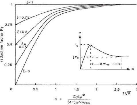
(28) Thèse de Insan Kamil, Université de Lille, 2019. CHAPTER I: STATE OF ART The shaft compression occurs during loading, and the deflection of pile can be estimated (Fleming, 2008). The movement due to slip occurs 0.5 to 2% of the pile diameter in clay and 0.2% in the sand where It starts at Pslip of pile load. The ratio between Pslip and ultimate shaft capacity Qs usually is taken between 0.5 to 0.6 (Fleming,2008). It shows that the failure around the pile can occur at the load level which is lower than maximum axial friction. This phenomenon is related to the compressibility of the pile and rigidity (Murff, 1980). In the flexible pile, a failure is achieved gradually through the pile. The failure may occur at the top of soil surrounding the pile while at the lower layer of soil has not reached the failure yet. But for the rigid pile, the friction peaks are mobilised along the pile surrounding the pile at the same time. The behaviour of this mobilisation is shown in Figure I.10. Where the value of Rf is affected by the value of the flexibility ratio K.. Figure I.10. The progressive failure of along pile Randolph (1983) introduced the equation for the ratio of flexibility as equation I.4. 𝐾=(. Where,  w. (I.4). ) . is the relative movement from peak to resedual, d is diameter of pile, L is. lengh of pile and (EA)p is the parameter of modulus young and area of pile. In order to allow the progressive failure of the pile, the value of reduction factor should be applied to shaft pilecapacity base on peak value of shaft friction that is shown in Figure I.11.. 15 © 2019 Tous droits réservés.. lilliad.univ-lille.fr.

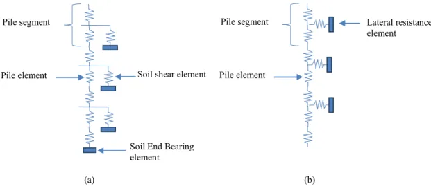
(29) Thèse de Insan Kamil, Université de Lille, 2019. CHAPTER I: STATE OF ART. Figure I.11. Variation of reduction factor with pile stiffness ratio I.3.2 Loads Transfer T-z Method The load-displacement relationship for axial load piles can be described through two loading mechanism, soil skin friction along the shaft and end-bearing of soil. The pile-capacity (Rc) is the ability of pile supporting the load which is a combination between shaft resistances (Rs) and bearing capacity (Rb) of the pile for axial load pile (Figure I.12.a and equation I.1). t Pile axial stiffness. z t. z Soil skin friction. Soil skin frictin (Rs). z t z. Soil end bearing (Rb). Q. Soil end bearing. z (b). (a). Figure I.12. The mechanism on axially monotonic load (a) transfer mechanism and (b) spring-mass model. 16 © 2019 Tous droits réservés.. lilliad.univ-lille.fr.

(30) Thèse de Insan Kamil, Université de Lille, 2019. CHAPTER I: STATE OF ART The shaft resistances (Rs) is total resistance along the pile calculated from equation I.3 where 𝑞 is unit load transfer in skin friction at segment i (normally varies with depth),ℎ is length at segment i and 𝑃𝑖 is perimeter of pile at segment i. the bearing resistance (Rb) is calculated from equation I.2 where 𝑞 is unit end-bearing resistance and 𝐴 is cross section area of pile. For an open tube pile, there are two condition of pile in bearing capacity mechanism which are plugged and unplugged condition (Figure I.13). The plugged condition (Figure I.13.a) happen when the open tube on tip of pile is compacted with the soil then the load transfer mechanism using full cross section area (Aplugged). And for unplugged condition (Figure I.13.b) consist of soil against the pile cross section area and internal skin friction (𝑞. ). ,. from the soil movement inside the shaft of pile. The equation I.5 is used for plugged condition (Rb,plugged), and the equation I.6 is used for unplugged condition (Rb,plugged).. (b). (a). Figure I.13. End bearing resistance considering (a) plugged condition and (b) unplugged condition. Where, 𝐴. ,. 𝑅. ,. 𝑅. ,. =𝑞 𝐴. (I.5). ,. =𝑞 𝐴. ,. + 𝑞. ,. 𝐴. (I.6). ,. is unplugged cross section area at the pile toe and 𝐴. ,. is surface. area of the pile segment inside the shaft interior in contact with soil in shear. On T-z curve method, the stress-strain relationship can be described through three loading mechanisms (Figure I.14) that are an axial deformation of the pile, soil skin friction and soil end-bearing. Springs present the interaction between pile and soil, the mobilisation of shaft friction described by non-linear springs distributed along the shaft and single spring at the base. The pile is divided into several segments due to the axial stiffness. The equation for the load transfer of external force on pile taken from the reaction at skin friction and pile deformation, the equilibrium of force can be seen at free body diagram of pile segment at depth z in Figure I.14. 17 © 2019 Tous droits réservés.. lilliad.univ-lille.fr.

(31) Thèse de Insan Kamil, Université de Lille, 2019. CHAPTER I: STATE OF ART. Qz uz z. dz. . Qz+dQz Figure I.14. Free body diagram of pile segment While the load applied on the segment, the reaction from shaft friction and internal pile force balance the load and then deformation occurs (uz). These situation expressed by the following equation: 𝑄 = 𝑄 + 𝑑𝑄 + .C.dz −. (I.7). = . C. (I.8). And the following equation for axially loaded beam describes the development of internal force in pile due to deformation, (I.9). 𝑄 = −𝐸𝐴 where, 𝑄 = internal pile force at depth z = soil unit friction at depth z C = circumference of pile at depth z E = Modulus elasticity of pile at depth z A = Cross section area of pile at depth z uz = Displacement of pile segment at depth z. Substitution the equation I.8 which is differentiated by z into equation I.9 yields to be the governing equation for the pile and soil as the following equation, 𝐸𝐴. = . C. . C − 𝐸𝐴. (I.10) (I.11). =0. In this method, the force which is produced by the unit weight of pile is negligible.. 18 © 2019 Tous droits réservés.. lilliad.univ-lille.fr.

(32) Thèse de Insan Kamil, Université de Lille, 2019. CHAPTER I: STATE OF ART Predicting Pile Axial Behaviour by Frank & Zhao method (Pressure Meter Test) The Pressure-meter test, which is different with other in situ test such as SPT (standard penetration test) or CPT (cone penetrometer test), is an in-situ testing method used to achieve a quick measure of the in-situ stress-strain relationship of the soil. In principle, the Pressuremeter test is performed by applying pressure to the sidewalls of a borehole and observing the corresponding deformation. There are two main parameters characterize the soil at each tested layer, in ASTM-1987 present a Pressure-meter modulus (Em) and limit pressure (Plm). The value of Em and Plm are described in a graph according to depth of soil followed by the description of soil type (Figure I.15).. Figure I.15. Example of Pressure-meter Test result Frank and Zhao (1982) uses the pressure meter approach in load to express the transfer method (T-z and P-y). The settlement p in pile tip is given by; 𝑧 =. . (I.12). 𝑞. Where, B is the diameter of the pile, qp is the pile tip pressure (with qp<qL). The skin friction qsi is mobilised during the settlement at each pile element (Figure I.16).. 19 © 2019 Tous droits réservés.. lilliad.univ-lille.fr.

(33) Thèse de Insan Kamil, Université de Lille, 2019. CHAPTER I: STATE OF ART 𝑧 =. (I.13). 𝑞. . And the sloop is controlled by ks for the T-z curve and kb for the P-y curve. Both ks and kb are the functions of the Pressure-meter modulus Em, which is governed by equation I.14 and I.15 For fine soils. 𝑘 = 2.0. For granular soil 𝑘 = 0.8. (I.14). 𝑎𝑛𝑑 𝑘 = 11. (I.15). 𝑎𝑛𝑑 𝑘 = 4.8.  . qs. q. ks/5. qs/ . . 0. q . . ks 6. . . (b).  Q. q . Kb/5. Qb/. . 0. q. Kb. . 6. . . (c). (a). Figure I.16. (a) Load-Transfer mechanism (b) the T-z curve (c) the q-z curve (after Frank and Zhao,1982) Since 1993, The calculating rules of pile-capacity from Pressure-meter test adopted from the new code of practice for foundations (MELT, 1993) known as the Fascicule 62-V. Bustamante et Gianeselli (2006) proposed the possibility of installation technique that made the possibility of re-adjusting the parameter of calculation of the axial limit coefficient. They proposed from 17 categories of the pile in Fascicule 62-V into 20 categories which have been grouped into eight classes. Burlon et al. (2014) revised the previous calculation that presented by Bustamante et Gianeselli (2006). The revision proposed for compliance in France standard with the requirements of Eurocode 7. The standard is relating to the dimensioning of the deep foundation NF P 94-262 (AFNOR,2012). Generally, the bearing capacity of the pile is expressed by equation I.16. But to express the value of Rb (tip bearing capacity) and Rs (shaft resistance) with PMT result are; 20 © 2019 Tous droits réservés.. lilliad.univ-lille.fr.

(34) Thèse de Insan Kamil, Université de Lille, 2019. CHAPTER I: STATE OF ART. (I.16). 𝑅𝑏 = 𝐴 𝑘𝑝 𝑃𝑙𝑒 ∗ Where A kp. = the pile tip area, where for steel driven piles are illustrated on Figure I.17. = the tip bearing factor. Ple*= the net equivalent Menard limit pressure under and around the pile tip 1 𝑏 + 3𝑎 𝐵 𝑎 = 𝑚𝑎𝑥 ; 0,5 2 𝑃𝑙𝑒 ∗ =. (I.17). 𝑃𝑙 ∗ (𝑧)𝑑𝑧. 𝑏 = 𝑚𝑖𝑛{𝑎; ℎ} Where h = the thickness of soil that is contained the carrier formation (resisting layer). a = the limit above the pile tip b = the limit below the pile tip B = Diameter of pile D = Depth of pile Pl. Pile. D h. b. 10 B B. 3a B. z. Resisting layer. (a). (b). Figure I.17. Model of the full pile (a) model of the base of pile (b) 1 𝑃𝑙 ∗ (𝑧)𝑑𝑧 𝑃𝑙𝑒 ∗ Where, Def = effective depth of pile 𝐷. (I.18). =. When the value of Def/B is bigger then 5 and kp is equal to kpmax where the value is depend on soil type and pile class (table II.1). If the value of Def/B is less then 5, use equation I.19 for the value kp, as described at Figure I.18.. 21 © 2019 Tous droits réservés.. lilliad.univ-lille.fr.

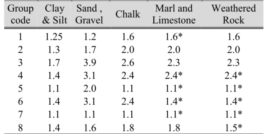
(35) Thèse de Insan Kamil, Université de Lille, 2019. CHAPTER I: STATE OF ART − 1.0) 𝐷 (I.19) 5 𝐵 At least, the embedded pile is equal to 3 times of diameter or 1,5 meters depth for the pile 𝑘 = 1.0 +. (𝑘. with the diameter greater than 0,5 meter. Kp Kp,max. 1 Def/B. 5. Figure I.18. Value of kp and Def/B Table I.4. Value for the tip bearing resistance factor kp,max for Def  5 (Burlon et al, 2014) Group Clay Sand , Marl and Weathered Chalk code & Silt Gravel Limestone Rock 1 2 3 4 5 6 7 8. 1.25 1.3 1.7 1.4 1.1 1.4 1.1 1.4. 1.2 1.7 3.9 3.1 2.0 3.1 1.1 1.6. 1.6 2.0 2.6 2.4 1.1 2.4 1.1 1.8. 1.6* 2.0 2.3 2.4* 1.1* 1.4* 1.1* 1.8. 1.6 2.0 2.3 2.4* 1.1* 1.4* 1.1* 1.5*. * A higher kp value can be used but must be proven by a load test. The ultimate skin friction is expressed by equation I.20. 𝑅𝑠 = 𝐴. (I.20). 𝐴 𝑞. (I.21). = 𝑃 .ℎ. Where, Asi is the side surface area at segment i, Pi is the perimeter of pile and the developed perimeter for calculation is illustrated on Figure I.19, and hi is thickness of segment at segment i,.. 22 © 2019 Tous droits réservés.. lilliad.univ-lille.fr.

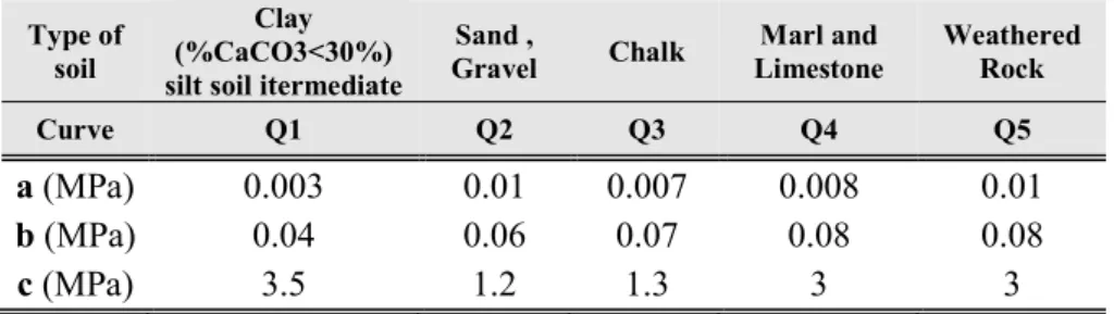
(36) Thèse de Insan Kamil, Université de Lille, 2019. CHAPTER I: STATE OF ART And, qsi is the ultimate unit skin friction at segment i where the value gives empirically considering the category of the pile, type of soil and pressure limit pl*. The expression for unit skin friction at equation I.23. where the minimum value from both calculations are taken. 𝑞 = 𝑀𝑖𝑛 {( 𝑓. 𝑓. (𝑝 ∗), (𝑞. (𝑝 ∗) = (𝑎 + 𝑏 . 𝑝 ∗)(1 − 𝑒. (I.22). )}. (I.23). . ∗. The parameter of fsoil are defined by three parameters ai, bi and ci where the value depends on the soil type (presented on table I.5 and Figure I.19). These parameters and the installation factor soil-pile (table I.6) are adjusted to optimize functions of the ratio of the calculated values to the measured values for the three quantities of Rb, Rs and Rc. The maximum Value ultimate skin friction qs-max for each soil type and installation methods are presented in table I.7. Table I.5. Selecting the Qi line to obtain the limit unit skin friction value qs (Burlon et al,2014) Type of soil. Clay (%CaCO3<30%) silt soil itermediate. Sand , Gravel. Chalk. Marl and Limestone. Weathered Rock. Curve. Q1. Q2. Q3. Q4. Q5. a (MPa) b (MPa) c (MPa). 0.003 0.04 3.5. 0.01 0.06 1.2. 0.007 0.07 1.3. 0.008 0.08 3. 0.01 0.08 3. 160. Q1 Q2 Q3 Q4 Q5. 140. sol(kPa). 120 100 80 60 40 20 0 0. 1. 2. 3. Pl (MPa). 4. 5. 6. 7. Figure I.19. Friction curve fsoil(pl*) 23 © 2019 Tous droits réservés.. lilliad.univ-lille.fr.

(37) Thèse de Insan Kamil, Université de Lille, 2019. CHAPTER I: STATE OF ART. Table I.6. Value of installation factor soil-pile (Burlon et al,2014 ) No. Installation methods. Clay (%CaCO3<30%) silt soil itermediate. Sand , Chalk Gravel. Marl and Weathered Limestone Rock. 1. Pile or barrette bored in dry. 1.1. 1. 1.8. 1.5. 1.6. 2. Pile or barrette bored with slurry. 1.25. 1.4. 1.8. 1.5. 1.6. 3. Bored and cased pile (permanent casing). 0.7. 0.6. 0.5. 0.9. 0.9. 4. Bored and cased pile (recoverable casing). 1.25. 1.4. 1.7. 1.4. 1.6. 5. Dry bored pile /or slurry bored piles with grooved socket /or pier (3 types). 1.3. 1.4. 1.8. 1.5. 1.6. 6. Bored pile with a single or a double rotation CFA (2 types). 1.5. 1.8. 2.1. 1.6. 1.6. 7. Screwed case in place. 1.9. 2.1. 1.7. 1.7. 1.7. 8. Screwed piles with cashing. 0.6. 0.6. 1. 0.7. 0.7. 9. Pre-cast or pre-stressed concrete driven pile (2 types). 1.1. 1.4. 1. 0.9. 0.9. 10. Coated Driven Pile (concrete, mortar, grout). 2. 2.1. 1.9. 1.6. 1.6. 11. Driven Cast-in-Place Pile. 1.2. 1.4. 2.1. 1. 1. 12. Driven Steel Pile, Closed End. 0.8. 1.2. 0.4. 0.9. 0.9. 13. Driven Steel Pile, Open End. 1.2. 0.7. 0.5. 1. 1. 14. Driven H Pile. 1.1. 1. 0.4. 1. 0.9. 15. Driven Grouted H Pile. 2.7. 2.9. 2.4. 2.4. 2.4. 16. Driven Sheet Pile. 0.9. 0.8. 0.4. 1.2. 1.2. 17. Micropile Type I. 1.25. 1.4. 1.8. 1.5. 1.6. 18. Micropile Type II. 1.25. 1.4. 1.8. 1.5. 1.6. 19. SGP Micropile (Type III) / or SGP Pile. 2.7. 2.9. 2.4. 2.4. 2.4. MRP Micropile (Type IV) / or MRP Pile. 3.4. 3.8. 3.1. 3.1. 3.1. 20. Note. For the categories 9 to 16, the above value are multiplied by 0.75 when the piles are vibro-driven instead of being driven.. 24 © 2019 Tous droits réservés.. lilliad.univ-lille.fr.

(38) Thèse de Insan Kamil, Université de Lille, 2019. CHAPTER I: STATE OF ART. Figure I.20. Area A and perimeter P to be used for open-end steel piles & sheet piles Table I.7. The maximum Value ultimate skin friction qs-max Value in kPa No. Instalation methods. Silt and clay, percentage Sand , Marl and Weathered Calcium carbonate Chalk Gravel Limestone Rock (CaCO3) < 30%. 1 Pile or barrette bored in dry. 90. 90. 200. 170. 200. 2 Pile or barrette bored with slurry 3 Bored and cased pile (permanent casing) 4 Bored and cased pile (recoverable casing) 5 Dry bored pile /or slurry bored piles with grooved socket /or pier (3 types) 6 Bored pile with a single or a double rotation CFA (2 types) 7 Screwed case in place. 90. 90. 200. 170. 200. 50. 50. 50. 90. ---. 90. 90. 170. 170. ---. 90. ---. ---. ---. ---. 90. 170. 200. 200. 200. 130. 200. 170. 170. ---. 8 Screwed piles with cashing. 50. 90. 90. 90. ---. 9 Pre-cast or pre-stressed concrete driven pile (2 types) 10 Coated Driven Pile (concrete, mortar, grout) 11 Driven Cast-in-Place Pile. 130. 130. 90. 90. ---. 170. 260. 200. 200. ---. 90. 130. 260. 200. ---. 12 Driven Steel Pile, Closed End 13 Driven Steel Pile, Open End. 90. 90. 50. 90. ---. 90. 50. 50. 90. 90. 14 Driven H Pile. 90. 130. 50. 90. 90. 15 Driven Grouted H Pile. 200. 380. 320. 320. 320. 16 Driven Sheet Pile. 90. 50. 50. 90. 90. 25 © 2019 Tous droits réservés.. lilliad.univ-lille.fr.

(39) Thèse de Insan Kamil, Université de Lille, 2019. CHAPTER I: STATE OF ART I.3.3 Loads Transfer P-y Method The most application used for lateral deflection analysis of pile is the P-y method. This method has been widely used because represents the calibration of actual conditions obtained from the full-scale test. Figure I.21.a, the cylindrical pile under lateral load, shows that the distribution of unit normal stress around the pile is uniform before displacement occurs (Figure I.21.b). When the deflection occurs at the distance y1 and the depth z1, the distribution of stress looks like Figure I.21.c. By resisting force (P1) at the opposite direction of the load which the stress decreases on the backside of the pile and increases on the front and also at the left and right side of the pile which has both normal and shearing stress as the displaced soil tries to move around the pile. Px M. H z. y1. z1 P1. y1 (b). (a). (c). Figure I.21. Unit stress distribution in lateral load The P-y method defines the relationship between lateral load and deflection which occurs between soil and pile described in a curve. p, unit lateral load. cohesive soil. cohesioless soil. y, deflection. Figure I.22. Behavior of P-y curve (Coduto,1994). 26 © 2019 Tous droits réservés.. lilliad.univ-lille.fr.

(40) Thèse de Insan Kamil, Université de Lille, 2019. CHAPTER I: STATE OF ART The axis-p is unit lateral load, and the axis-y is a lateral deflection of the pile. The behaviour of P-y curve showed in Figure I.22 which is describing the relationship on the P-y curve for cohesive soil and cohesionless soil. The influence parameter on the P-y curve is the type of soil, type of load (short/long term, monotonic or dynamic), the diameter of the pile, shaft friction, depth of pile, installation method and interaction pile to pile in a group of the pile. The analysis in the P-y method is done by considering the behaviour of P-y curve throughout the pile (Figure I.23). It can be solved by Finite difference analysis which divides the pile into n segments. For the analysis, the boundary condition is needed. There is two boundary condition at the tip of the pile, shear stress and zero moments. Boundary condition on top of pile depends on the type of connection of piles head with pile-cap (unrestrained/free-head pile and restrained/fix-head pile), as follows: - Unrestrained/free-head pile, horizontal shear strength (V) and moment (M) are determined. On piles head, there is rotation and deflection (St≠0 and yt≠0) - Restrained/fix-head pile, horizontal shear strength (V) and slope (St) are defined. For the first assumption, St is null, but it can have value.. p Lateral component moving soil. of y-ysoil p. Pile Bending stiffness (EI). y-ysoil. Soil Lateral resistance. p y-ysoil. Sliding Surface p. y-ysoil. Figure I.23. Pile segment discretization pile element and soil element. The differential equation for a beam column is described by equation I.24 solving the implementation of the P-y method. E 𝐼 where, y. +P. +E. 𝑦−𝑊 =0. (I.24). = displacement of pile. E 𝐼 = bending stiffness of pile 27 © 2019 Tous droits réservés.. lilliad.univ-lille.fr.