Ordre stochastique des produits scalaires avec application

يملعلا ثحبلاو لياعلا ميلعتلا ةرازو

راـتمخ يـجبا ةـعماج

ةـباـنع

Université Badji Mokhtar

Annaba

Badji Mokhtar University –

Annaba

Faculté des Sciences

Département de Mathématiques

Laboratoire LaPS

THESE

Présentée en vue de l’obtention du diplôme de

Doctorat en Mathématiques

Option : Probabilités et Statistique

Ordre stochastique des produits scalaires avec application

Par:

BOUHADJAR Meriem

DIRECTEUR DE THESE :

ZEGHDOUDI Halim M.C.A U.B.M.Annaba

CO-DIRECTEUR DE THESE:

REMITA Mohamed Riad Prof. U.B.M.Annaba

Devant le jury

PRESIDENT : BOUTABIA Hacène

Prof.

U.B.M.Annaba

EXAMINATEUR : HADJI Mohamed Lakhdar

M.C.A

U.B.M. Annaba

EXAMINATEUR :

BRAHIMI Brahim

M.C.A

U. Biskra

.اهتاقيبطتو راطخلأل ةيئاوشعلا تابيترتلا نع ةماع ةحمل حرتقن ةحورطلأا هذه يف

مب

ىلإ ةفاضإ ،نيمأتلا ةظفحمل دئاوفلا ةميق ميظعت ةلكشم ىلإ قرطتنس قدأ ىنع

ضعبب اهتقلاعو نيمأتلا ةصيلوب تاعاطتقاو دودحل لثملأا عيزوتلا لوح تاقيبطت

ةيراوتكلإا عيضاوملا

ىرخلأا

:اهنم

ةنراقم

copulas

جذامن ،

نع

رطاخملا

،نيمأتلا ةداعإ دوقعو ةيعامجلاو ةيدرفلا

إ

.خل

لا تاملكلا

ةيسيئر

:

Comonotonicité

بيترتلا ،

بدحملا

تاعاطتقاو دودح ،

.نيمأتلا ةصيلوب

Contents

List of Figures 3

1 Introduction 8

2 Preliminaries and Notations 12

2.1 Utility function . . . 13 2.2 Majorization Order . . . 15 2.3 Arrangement Increasing . . . 17 2.4 Value-at-Risk . . . 19 2.4.1 Tail Value-at-Risk . . . 20 2.5 Sotachastic orders . . . 21 2.5.1 Stochastic Dominance . . . 21 2.5.2 Sotachastic order . . . 23

2.5.3 Convex ordering random variables . . . 24

2.5.4 Lorenz Order . . . 28

2.6 Inverse distribution functions . . . 30

3 Comonotonicity 35 3.1 Comonotonic sets and random vectors . . . 35

3.2 Examples . . . 42

3.3 Sums of comonotonic random variables . . . 44

3.4 The New Results . . . 52

3.4.1 Convex bounds and the comonotonic upper bound for SN . . . 52

4 Policy Limits and Deductibles 56 4.1 Policy limits with unknown dependent structures . . . 57

4.2 Policy deductibles with unknown dependent structures . . . 59

4.3 Some examples and Application . . . 61

4.3.1 Lower Bound Approximations of the Distribution Sum of Ran-dom Variables with Convex Ordering . . . 62

4.3.2 Individual and collective risk model . . . 65

4.3.3 Reinsurance contracts . . . 65

4.3.4 Dependent portfolios increase risk . . . 66

4.3.5 Applications of the theory of comonotonicity . . . 66

4.3.6 Comparison of two families of copulas . . . 68

5 Appendix 73

List of Figures

5.1 Graphical de…nition of F_X1; F_X1+ and F_X1( ): . . . 75 5.2 A continuous example with n = 3: . . . 75 5.3 A discrete example. . . 76

BIBLIOGRAPHIE PERSONNELLE

Articles publiés

1. Bouhadjar, M. Zeghdoudi, H. Remita, M.R, Ordering of the Optimal Allocation of Policy Limits in general model. European Journal of Scienti…c Research, ISSN 3 Volume 134, 317-324 (2015).

2. Bouhadjar, M. Zeghdoudi, H. Remita, M.R, Stochastic Order Relationship and Its Applications in Actuarial Science. Global Journal of Pure and Applied Mathematics, ISSN 0973-1768 Volume 11, Number 6, pp. 4395-4403 (2015).

3. Bouhadjar, M. Zeghdoudi, H. Remita, M.R, On Stochastic Orders and Applica-tions : Policy Limits and Deductibles. Applied Mathematics & Information Sciences, Volume 10, Number 4, pp. 1-8 Published online: (1 Jul 2016).

Introduction générale en français

La science actuarielle moderne et la théorie de risque jouent un rôle important dans l’économie et la …nance. Un des principaux objectifs de la profession actuarielle est la comparaison de variables aléatoires (risques). Habituellement, le critère

probab-iliste « moyenne - variance» ne su¢ t pas toujours à comparer des variables aléatoires. Cependant, il arrive souvent qu’on possède des informations plus détaillées en utilisant les fonctions de répartition des variables aléatoires pour les comparés. Pour cela, il est

préférable de faire une comparaison basée sur les distributions que celle basée unique-ment sur deux statistiques. La méthode utilisée pour comparer deux distributions est nommée « ordre stochastique» . Tout d’abord, nous donnons un aperçu historique

de ce terme. Depuis les années 70, le concept de dominance stochastique, introduit par Rothschild-Stieglitz, permet de comparer des distributions de probabilité. Plus récemment, les ordres stochastiques qui généralisent la dominance stochastique sont

utilisés de façon accélérée dans plusieurs domaines, notamment la …nance, science actuarielle et l’économie. En faite, des ordres stochastiques particuliers aient déjà été étudiés par Karamata en 1932, par Lehmann en 1955, et par Littlewood et Polya

en 1967. En…n, les premières études presque complètes des ordres stochastiques ont été données par Stoyan dans les années 1977 et 1983, et par Mosler en 1982. En …n-ance et en économie, une des raisons principales pour comparer des variables aléatoires

(risques) en utilisant des ordres stochastiques est le fait que ces derniers utilisent toute l’information sur la fonction de répartition a…n d’établir une comparaison adéquate

entre deux variables aléatoires.

Notre travail est structuré de la manière suivante :

Le chapitre 2 présente et examine de façon systématique les ordres stochastiques

univariés les plus utilisés dans la littérature. Par ailleurs, des dé…nitions, notations et propriétés sont établies. Par exemple, la fonction d’utilité, ordre de majorisation, valeur at risque, et la fonction de distribution inverse.

De ce fait, le chapitre 3 traite la comonotonicté, à savoir les ensembles comono-tones, les vecteurs aléatoires comonocomono-tones, la somme comonotone des variables aléatoires et les bornes convexes pour la somme des variables aléatoires.

En…n, le dernier chapitre présente la contribution originale de notre travail dont nous introduisons un nouveau modéle de l’allocation optimale des limites de police et des déductibles. Il s’agit d’une extension et complémemt du résultat de Cheung

[6], Hua and Cheung [29] and Zhuang et al.[58]. Des applications sur l’allocation optimale des limites de police et des déductibles sont obtenus, et quelques relations avec d’autres sujets actuariels principaux (comparaison des copules, les modèles de

risque individuels et collectifs, des contrats de réassurance, etc.) sont également étudiés.

Cette contribution est couronnée par (03) publications scienti…ques dans des

re-vues de renommées internationales à savoir:

Bouhadjar, M. Zeghdoudi, H. Remita, M.R, Ordering of the Optimal Allocation

ISSN 3 Volume 134, 317-324 (2015).

Bouhadjar, M. Zeghdoudi, H. Remita, M.R, Stochastic Order Relationship and Its Applications in Actuarial Science. Global Journal of Pure and Applied

Math-ematics, ISSN 0973-1768 Volume 11, Number 6, pp. 4395-4403 (2015).

Bouhadjar, M. Zeghdoudi, H. Remita, M.R, On Stochastic Orders and Applic-ations : Policy Limits and Deductibles. Applied Mathematics & Information Sciences, Volume 10, Number 4, pp. 1-8 Published online: (1 Jul 2016).

Chapter 1

Introduction

Modern actuarial science and risk theory play a crucial role in the economy and …nance. One of the principal objectives of the actuarial profession is the comparison of random variables (risks). Usually, the probabilistic criterion « mean - variance»

is not always enough to compare random variables. However, it often happens that we have more detailed information by using the distribution functions of the random variables for compared.

This work is innovative in many respects. It integrates the theory of stochastic or-ders, one of the methodological cornerstones of risk theory and the theory of stochastic dependence, which has become increasingly important as new types of risks emerge.

More precisely, risk measures will be used to generate stochastic orderings, by identi-fying pairs of risks about which a class of risk measures agree. Stochastic orderings are then used to de…ne positive dependence relationships.

In several works, orderings of optimal allocations of policy limits and deductibles were established by maximizing the expected utility of wealth of the policyholder. In this work, we study the problems of optimal allocation of policy limits and deductibles

for general model,by using some characterizations of stochastic ordering relations, we reconsider the new general model and obtain some new results on orderings of optimal allocations of policy limits and deductibles. To this end, we obtain the ordering of

the optimal allocation of policy limits, deductibles for this model and we extend the above results in Cheung (2007; 2008).

We consider for the following model :

SN = X1f (Y1) + X2f (Y2) + ::: + Xnf (Yn) (M1)

where :Yi = iTi, SN is total discounted loss, Xi are loss due to the i-th risk, Ti are

time of occurrence of i-th insured risk and i are discount rate capture the impact of

…nancial environment (Xi; Ti are independent non-negative random variables and i

are non-random numbers). Also, we will make the following assumptions 1. f (Yi) 0;8Yi and lim f (Yi)

Yi!1

= 0:

2. f (Yi) is decreasing and convex function.

3. Y1; Y2; :::; Yn are mutually independent.

4. A policyholder exposed to risks X1; X2; :::; Xn is granted a total of l dollars (l > 0)

as the policy limit with which (s)he can allocate arbitrarily among the n risks.

scales of the losses while f (Yi) characterize the chances of the losses.

In this situation, if some risk occurs, the insurer will make the payment right

after the event of the loss and the insurance coverage for this risk will terminate. However the insurance coverage for the other risks is still in e¤ect. If (l1; :::; ln) are

the allocated policy we have 8i : li 0 and n

X

i=1

li = l. When l is n-tuple admissible

and An(l) denote the class of all such n-tuples. If l = (l1; :::; ln) 2 An(l) is chosen,

then the discounted value of bene…ts obtained from the insurer would be

n

X

i=1

(Xi^ li) f (Yi) (1.1)

If we take expected utility of wealth as the criterion for the optimal allocation, then the problem of the optimal allocation of policy limits is

Problem L : max l2An(l)E " u w n X i=1 [Xi (Xi^ li)] f (Yi)) !# : (1.2)

where u is the utility function of the policyholder and w is the wealth (after premium). Similarly, instead of policy limits, the policyholder may be granted a total of d dollars

(d > 0) as the policy deductible with which (s)he can allocate arbitrarily among the n risks. If d = (d1; :::; dn) 2 An(d) are the allocated deductibles, then 8i : di

0;

n

P

i=1

di = d, and the discounted value of bene…ts obtained from the insurer would be

n

X

i=1

Chapter 2

Preliminaries and Notations

In this chapter, we will present some de…nitions like: Utility function, Majorization Order, Arrangement Increasing. . . etc.

Throughout this work, we de…ne In = f(a1; :::; an) 2 Rn : a1 ::: ang and

Dn = f(a1; :::; an) 2 Rn : a1 ::: ang. In addition, we noted that x[i] and x(i)

are the i-th largest and the i-th smallest element of x respectively. The notation x " will be used to indicate the increasing rearrangement (x(1); :::; x(n))2 In and x # will

be used to indicate the decreasing rearrangement (x[1]; :::; x[n]) 2 Dn for any vector

x = (x₁; :::; xn)2 Rn. We represent a permutation of the set f1; 2; :::; ng by , then

2.1

Utility function

In economics, utility is a measure of preferences over some set of goods and ser-vices. A utility function, u(x), can be described as a function which measures the value, or utility, that an individual (or institution) attaches to the monetary amount

x. Throughout this work we assume that a utility function satis…es the conditions

u0(x) > 0 and u00(x) < 0: (2.1)

Mathematically, the …rst condition says that u is an increasing function, while the

second says that u is a concave function. Simply put, the …rst states that an individual whose utility function is u prefers amount y to amount z provided that y > z, that is the individual prefers more money to less! The second states that as the individual’s

wealth increases, the individual places less value on a …xed increase in wealth. An individual whose utility function satis…es the conditions in (2:1) is said to be risk averse, and risk aversion can be quanti…ed through the coe¢ cient of risk aversion

de…ned by

r(x) = u

00_(x)

u0_(x) (2.2)

The expected utility criterion

Decision making using a utility function is based on the expected utility criterion.

This criterion says that a decision maker should calculate the expected utility of resulting wealth under each course of action, then select the course of action that gives the greatest value for expected utility of resulting wealth. If two courses of

action yield the same expected utility of resulting wealth, then the decision maker has no preference between these two courses of action. To illustrate this concept, let us consider an investor with utility function u who is choosing between two investments

which will lead to random net gains of X1 and X2 respectively. Suppose that the

investor has current wealth W , so that the result of investing in Investment i is W + Xi f or i = 1 and 2. Then, under the expected utility criterion, the investor

would choose Investment 1 over Investment 2 if and only if

E[u(W + X1)] > E[u(W + X2)]

Further, the investor would be indi¤erent between the two investments if

E[u(W + X1)] = E[u(W + X2)]

Types of utility function

It is possible to construct a utility function by assigning di¤erent values to di¤erent levels of wealth. In the following table we consider some mathematical functions which

may be regarded as having suitable forms to be utility functions.

T ypes F orm U se

Exponential u(x)= expf xg; where >0 Decisions do not depend on the individual0s wealth

Quadratic u(x)= log x; f or x>0 and >0 Restricted by the constraint x<₂1; which is required u0_(x)>0

Logarithmic u(x)= log x; f or x>0 and >0 F or positive values of x

2.2

Majorization Order

De…nition 2.1 ([6]) Given any two vectors a; b_{2 R}n;

1. b is said to be majorized by a (denoted by b a),if 8 > > < > > : Pn i=1b[i] = Pn i=1a[i] Pm i=1b[i] Pm i=1a[i] m = 1; :::; n 1: (2.3)

2. b is said to be weakly majorized by a (denoted by b a); if

m X i=1 b[i] m X i=1 a[i]; m = 1; :::; n: (2.4)

If b a, then b is also said to be smaller than a in the majorization order. In literature, there are two di¤erent versions of weak majorization. The de…nition given

above is commonly known as weak submajorization. We refer to Marshall and Olkin (1979) and Tong (1980) as standard references for the theory of majorization.

The following is the de…nition of a T-transform, which is a very useful tool in the

study of the majorization order. After the de…nition, we will collect some useful properties of a T-transform.

De…nition 2.2 (_{[6]) A T-transform is a kind of linear transformation (from R}n to Rn_{) whose transformation matrix has the form}

T = I + (1 )Q (2.5)

where 0 1, I is the identity matrix and Q is a permutation matrix that interchanges two coordinates.

Lemma 2.3 ([6]) If b a, then b can be derived from a by successive applications of a …nite number of T-transforms, and any T-transform can preserve the majorization order. i.e., b T (a) a; where T is a T-transform.

For a proof of this result, we refer to Marshall and Olkin (1979) and Hardy et al.(1934; 1952). Since each T-transform will only modify two coordinates in a vector,

Lemma (2:3) shows that it is often su¢ cient to check the case n = 2 in proving results concerning majorization order. The next lemma provides a re…nement when both a and b are in In:

Lemma 2.4 ([6]) Suppose that a and b are vectors in _In. If b a, then b can be

derived from a by successive applications of a …nite number of T-transforms of the

form

T (a) = (a1; :::; ai 1; ai+(1 )aj; ai+1; ::::; ::::; aj 1; aj+(1 )ai; aj+1; :::; an); (2.6)

where 1

2 1; so that T (a)2 In and b T (a) a:

Proof. _{If we change each I}n in the above result to Dn and keep the rest

un-changed, then it is a fact given in [40]. Since

a; b _{2 D}n; b a) a; b 2 In;and (2.7)

the result follows.

An interesting property of the above T-transform is that it not only preserves the majorization order but also preserves the ordering of the vector’s components.

Lemma 2.5 ([6]) If b a _{and a 2 I}n, then n X i=1 aix[i] n X i=1 bix[i] n X i=1 aix[n i+1] (2.8)

Lemma 2.6 ([6]) b a if and only if there exists a c such that c a and b c (i:e:; bi cif or each i)

Lemma (2:5) can be derived from the well-known rearrangement inequality; a proof is given in [41]. Lemma (2:6) characterizes the weak majorization order in

terms of the majorization order, its proof can be found in Marshall and Olkin (1979, page 123).

2.3

Arrangement Increasing

De…nition 2.7 (_{[6]) A function f : R}n

! R is said to be arrangement increasing [decreasing], if for all i and j such that 1 i < j n,

(xi xj)ff(x1; :::; xi; :::; xj; :::; xn) f (x1; :::; xj; :::; xi; :::; xn)g [ ]0: (2.9)

One major example is given by the joint density function of mutually independent random variables that are ordered by the likelihood ratio order.

Lemma 2.8 ([6]) If X1; :::; Xn are mutually independent and X1 lr ::: lr Xn;then

the joint density function of (X1; :::; Xn) is arrangement increasing.

De…nition 2.9 (_{[6]) A function g(x; ) : R}n _Rn_{! R is said to be an arrangement} increasing (AI ) function if

1. g is permutation invariant, i.e., g(x; ) = g(x ; ) for any permutation , and

2. g exhibits permutation order, i.e., g(x #; ") g(x_#; ) g(x_{#; #) for} any permutation .

The following lemmas give us two examples of AI functions. Proofs can be found in [6].

Lemma 2.10 (_{[29]) The function g : R}n

Rn ! R de…ned by g(x; ) = n X i=1 (xi i)+and g(x; ) = n X i=1 (xi^ i) (2.10) are an AI function.

Proofs of the following lemmas can be found in [29].

Lemma 2.11 ([29]) Suppose that the function _{(x; ) : R}2

! R is increasing both in x and . If the function

g(x; ) =

n

X

i=1

from Rn Rn to R is an AI function, then

^(x #; ") ^ (x #; ) ^ (x #; #) (2.11) for any permutation :

Lemma 2.12 (_{[29]) Suppose that the function (x; ) : R}2

! R is increasing in one variable and decreasing in the other. If the function

g(x; ) =

n

X

i=1

(xi; i)

from Rn Rn to R is an AI function, then

^(x #; #) ^ (x #; ) ^ (x #; ") (2.12) for any permutation :

2.4

Value-at-Risk

These last years, several experts saw importance of the quantiles of the probability distributions Since quantiles especially have an easy interpretation in practice of risk

management in the form of the concept of value-at-risk (VaR). This concept was introduced to answer the following question: how much can we expect to lose in one

day, week, year, with a given probability? The VaR is given in Jorion (2000). In the following de…nition we de…ned VaR .

De…nition 2.13 ([21]) Given a risk X and a probability level p_{2 (0; 1), the} corres-ponding V aR, denoted by V aR [X; p], is de…ned as

V aR [X; p] = F_X1(p) : (2.13)

Note that the VaR risk measure reduces to the percentile principle of Goovaerts,

De Vijlderand Hazendonck (1984).

2.4.1

Tail Value-at-Risk

A single VaR at a predetermined level p does not give any information about the thickness of the upper tail of the distribution function. This is a considerable shortcoming since in practice a regulator is not only concerned with the frequency

of default, but also with the severity of default. Also shareholders and management should be concerned with the question ‘how bad is bad?’ when they want to evaluate the risks at hand in a consistent way. Therefore, one often uses another risk measure,

which is called the tail value-at-risk (T V aR) and de…ned next.

De…nition 2.14 ([21]) Given a risk X and a probability level p, the corresponding

TVaR, denoted by T V aR [X; p] , is de…ned as

T V aR [X; p] = 1 1 p 1 Z p V aR [X; ] d ; 0 < p < 1: (2.14)

We thus see that T V aR [X; p] can be viewed as the ‘arithmetic average’ of the

2.5

Sotachastic orders

2.5.1

Stochastic Dominance

Stochastic dominance and risk measures

Stochastic dominance and VaRs In order to compare a pair of risks X and Y, it seems natural to resort to the concept of V aR, and to consider X as less

dangerous than Y if V aR [X; 0] V aR [Y ; 0]for some prescribed probability level

0. However, it is sometimes di¢ cult to select such an 0, and it is conceivable that

V aR [X; 0] < V aR [Y ; 0] and V aR [X; 1] > V aR [Y ; 1] simultaneously for two

probability levels 0 and 1. In this case, what can we conclude? It seems reasonable

to adopt the following criterion: we place X before Y if the V aRs for X are smaller than the corresponding V aRs for Y , for any probability level.

De…nition 2.15 Let X and Y be two rvs. Then X is said to be smaller than Y in stochastic dominance, denoted as X ST Y, if the inequality V aR [X; p] V aR [Y ; p]

is satis…ed for all p 2 [0; 1].

Standard references for ST are the books of Lehmann (1959), Marshall and Olkin

(1979), Ross (1983) and Stoyan (1983).

Stochastic dominance can also be characterized by the relative inverse distribution

function, de…ned as

It is nothing more than the V aR of X at probability level p = FY (x) :

Stochastic dominance and monotonicity An important characterization of

ST is given in the next result. It essentially states that if X ST Y holds then there

exist rvs ~X and ~Y, distributed as X and Y for which PrhX~ Y~i= 1. In such a case, ~

Y is larger than ~X according to Kaas et al.(2001, De…nition 10.2.1). This proposition shows that ST is closely related to pointwise comparison of rvs.

Proposition 2.16 Two rvs X and Y satisfy X ST Y if, and only if, there exist two

rvs ~X and ~Y such that X =dX, Y =~ dY~ and Pr

h ~

X Y~i = 1. For a proof, see Kaas

et al.(2001, Theorem 10.2.3). The construction of ~X and ~Y involved in Proposition (2:16) is known as a coupling technique (see Lindvall 1992). Proposition (2:16) can be rewritten as follows.

Proposition 2.17 Two rvs X and Y satisfy X ST Y if, and only if, there exists

a comonotonic random couple (Xc; Yc) such that Pr [Xc Yc] = 1, X =d Xc and

Y =dYc:

Stochastic dominance and stop-loss premiums The following result relates

ST to stop-loss transforms. (The function X (t) = E (X t)+ is called the

stop-loss transform of X (See Kaas 1993)).

Proposition 2.18 Given two rvs X and Y , X ST Y if, and only if, Y X is

Proof. Clearly, if X ST Y, FY FX is non-negative so that the result follows

from X(t) =

R+1

t FX( ) d : Now assume the non-increasingness of the di¤erence Y X: Di¤erentiating this expression with respect to t yields FX(t) FY (t) 0,

whence X ST Y follows.

It is interesting to give an actuarial interpretation for Proposition (2:18). It basically states that when X ST Y holds, the di¤erence between their respective stop-loss

premiums decreases with the level t of retention. Since

lim

t!+1 E (Y t)+ E (X t)+ = 0

we thus have that the largest di¤erence occurs for t = 0 (and equals E (Y ) E (X)) and that this di¤erence decreases with the level of retention. The pricing of

stop-loss treaties will thus lead to very di¤erent premiums for small retentions, but this di¤erence will decrease as the retention increases.

2.5.2

Sotachastic order

There are several references for stochastic orders include Denuit et al.(2002; 2005),

Kaas et al.(1994; 2001), Müller and Stoyan (2002), Shaked and Shanthikumar (1994; 2007). We assume all random variables are de…ned on a common probability space ( ; F; P) and all expectations mentioned exist.

De…nition 2.19 Let X and Y be two random variables,

convex order, decreasing convex order, convex order), denoted by X st Y (resp:

X icx Y; X dcx Y; X cx Y ), if

E[ (X)] E [ (Y )] (2.16)

for all increasing (resp. increasing convex, decreasing convex, convex) function :

2. X is said to be smaller than Y in the likelihood ratio order, denoted by X lr Y,

if

fX(x)gY(y) fX(y)gY(x) for all x y (2.17)

where fX and gY are the density functions of X and Y , respectively.

2.5.3

Convex ordering random variables

In this subsection we give the de…nition of the Stop-loss premium by E[(X d)+] = 1

Z

d

(1 FX(x))dx; 1 < d < +1: Hence, we use the notation S for the sum of the

random vector (X1; X2; :::; Xn) : S = X1 + X2 + ::: + Xn: Moreover, we will present

the convex order and his characterization using Stop-loss premium . We start by de…ne the Stop-loss order between random variables

De…nition 2.20 ([9]) (Stop-loss order). Consider two random variables X and Y . then X is said to precede Y in the stop-loss order sense, notation X st Y if and

only if X has lower stop-loss premiums than Y :

with (X d)+= max(X d; 0):

De…nition 2.21 ([9]) (convex order). Consider two random variables X and Y such

that E [ (X)] E [ (Y )] ; for all convex functions ;provided expectation exit. Then X is said to be smaller than Y in the convex order denoted as X cx Y.

De…nition 2.22 ([9]) (Convex order characterization using stop-loss premium). Con-sider two random variables X and Y . Then X is said to precede Y in convex order sense if and only if

E [X] = E [Y ] (2.19)

E[(X d)+] E[(Y d)+]; 1 < d < +1

Where

(X d)+ = max(X d; 0)

An equivalent de…nition can be derived from the following relation

E[(X d)+] E[(d X)+] = E(X) d

For the random variable Y the same relation is given by

E[(Y d)+] E[(d Y )+] = E(Y ) d

E [X] = E [Y ]

and

E[(X d)+] E[(Y d)+]; 1 < d < +1

hence

E[(d X)+] E[(d Y )+]

Therefore, a de…nition equivalent to the de…nition here is

E [X] = E [Y ]

E[(d X)+] E[(d Y )+]; 1 < d < +1

Properties of Convex Ordering of Random Variables

1. If X precedes Y in convex order sense i.e if X cx Y, then E [X] = E [Y ] and

V[X] V[Y ] ;where V [X] is variance of X: [9]

2. If X cx Y and Z is independent of X and Y then X + Z cxY + Z: [9]

3. Let X and Y be two random variables, then X cx Y ) X cx Y: [15]

4. Let X and Y be two random variables such that E [X] = E [Y ] : Then X cxY

5. The convex order is closed under mixtures: Let X; Y and Z be random variables such that [X j Z = z] cx [Y j Z = z] 8z in the support of Z. Then X cx Y:

[33]

6. The convex order is closed under Convolution: Let X1; X2; :::; Xm be a set of

independent random variables and Y1; Y2; :::; Ym be another set of independent

random variables. If Xj cx Yj;for i = 1; :::; m, then

Pm

j=1Xj cx

Pm

j=1Yj: [9]

7. Let X be a random variable with …nite mean. Then X + E [X] cx 2X: (It

su¢ ces to use the De…nition (2:22))

8. Let X1; X2; ::Xn and Y be (n + 1) random variables. If Xi cx Y; i = 1; :::; n;

thenPn_i=1aiXi cxY, whenever ai 0; i = 1; :::; nand

Pn

i=1ai = 1:(It su¢ ces

to use the property 6)

9. Let X and Y be two random variables. Then X cxY if and only if E [ (X; Y )]

E [ (Y; X)],8 2 cx where

cx= : R2 ! R : (X; Y ) (Y; X) is convex for all x 2 y : (2.20)

(It su¢ ces to use the De…nition (2:22))

10. Let X1 and X2 be a pair of independent random variables and let Y1 and Y2

be another pair of independent random variables. If Xi cx Yi, i = 1; 2 then

X1X2 cx Y1Y2. [9]

12. Let X; Y and Z be random variables such that X cx Y and Y cx Z; then

X cxZ: (It su¢ ces to use the De…nition (2:22))

13. If X lr Y and is any decreasing function, then (X) lr (Y ). [50]

14. Let X 2 Rn

+ and X1 lr ::: lr Xn are mutually independent. If b is weakly

majorized by a (denoted by b a) _{and a 2 I}n, then n P i=1 biXi icx n P i=1 aiXi. [29]

2.5.4

Lorenz Order

The Lorenz order is de…ned by means of pointwise comparison of the Lorenz

curves. These are used in economics to measure the inequality of incomes. More precisely, let X be a non-negative rv with df FX. The Lorenz curve LCX associated

with X is then de…ned by

LCX = 1 E (X) Z p =0 V aR [X; ] d , p_{2 [0; 1] :} (2.21)

In an economics framework, when X models the income of the individuals in some population, LCX maps p 2 [0; 1] to the proportion of the total income of the

popu-lation which accrues to the poorest 100p % of the popupopu-lation. An interpretation of LCX in insurance business is the following: LCX(p) can be thought of as being the

claim size. Lorenz order

Now, we de…ne the lorenz order

De…nition 2.23 ([9]) Consider two risks X and Y . Then, X is said to be smaller

than Y in the Lorenz order, henceforth denoted by X Lorenz Y, when LCX(p)

LCY (p) for all p2 [0; 1].

A standard reference on Lorenz is Arnold (1987). We mention that <3 in

Heil-mann (1985) is in fact Lorenz. We also mention that the Lorenz order is the k-order

introduced by Heilmann (1986) (see also Heilmann and Schröter 1991, Remark 5) Lorenz and Convex orders

There is a closely relation between the convex and Lorenz orders.

Property Given two risks X and Y ,

X Lorenz Y ,

X E [X] cx

Y

E [Y ]: (2.22)

Obviously, when E [X] = E [Y ], we have

X Lorenz Y , X cxY (2.23)

since the convex order is scale-invariant. It is worth mentioning that other approaches

to comparing rvs with unequal means via cxhave been proposed. The dilation order,

2.6

Inverse distribution functions

The cdf FX(x) = P[X x] of a random variable X is a right-continuous (further

abbreviated as r.c.) non-decreasing function with

FX( 1) = lim

x! 1FX(x) = 0; FX(+1) = limx!+1FX(x) = 1:

The usual de…nition of the inverse of a distribution function is the non-decreasing and left-continuous (l.c.) function F_X1(p) de…ned by

F_X1(p) = inf_{fx 2 R j F}X(x) pg ; p2 [0; 1] (2.24)

with inf ; = +1(sup ; = 1) by convention. For all x 2 R and p 2 [0; 1]; we have

F_X1(p) x_{, p} FX(x): (2.25)

In this work, we will use a more sophisticated de…nition for inverses of distribution functions. For any real p 2 [0; 1], a possible choice for the inverse of FX in p is any

point in the closed interval

[inf_{fx 2 R j F}X(x) pg ; sup fx 2 R j FX(x) pg] ;

where, as before, inf ; = +1, and also sup ; = 1: Taking the left hand border of this interval to be the value of the inverse cdf at p, we get F_X1(p).

F_X1+(p) = sup_{fx 2 R j F}X(x) pg ; p2 [0; 1] (2.26)

which is a non-decreasing and r.c. function. Note that F_X1(0) = _{1; FX}1+(1) = +₁ and that all the probability mass of X is contained in the interval F_X1+(0); F_X1(1) :

Also note that F_X1+(p) _{are …nite for all p 2 (0; 1). In the sequel, we will always use} p as a variable ranging over the open interval (0; 1), unless stated otherwise.

For any _{2 [0; 1] ; we de…ne the -mixed inverse function of F}X as follows:

F_X1( )(p) = F_X1(p) + (1 )F_X1+(p); p_{2 (0; 1) ;} (2.27)

which is a non-decreasing function. In particular, we …nd F_X1(0)(p) = F_X1+(p) and F_X1(1)(p) = F_X1(p). One immediately …nds that for all _{2 [0; 1] ;}

F_X1(p) F_X1( )(p) F_X1+(p); p_{2 (0; 1) :} (2.28)

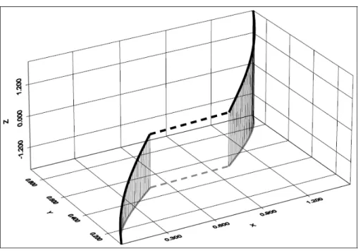
Note that only values of p corresponding to a horizontal segment of FX lead to

di¤er-ent values of F_X1(p); F_X1+(p) and F_X1( )(p): This phenomenon illustrated in …gure 5:1.

Now led d be such that 0 < FX(d) < 1: Then FX1(FX(d)) and FX1+(FX(d)) are

…nite, and F_X1(FX(d)) d FX1+(FX(d)). So for some value d 2 [0; 1] ; d can

be expressed as d = dF_X1(FX(d)) + (1 d)F_X1+(FX(d)) = F 1( d)

X (FX(d)) : This

implies that for any random variable X and any d with 0 < FX(d) < 1; there exists

an d2 [0; 1] such that F 1( d)

In the following theorem, we state the relation between the inverse didtribution func-tions of the random variables X and g (X) For a monotone function g:

Theorem 2.24 Let X and g (X) be real-valued random variables, and let 0 < p < 1:

(a) If g is non-decreasing and l.c., then

F_g(X)1 (p) = g F_X1(p) : (2.29)

(b) If g is non-decreasing and r.c., then

F_g(X)1+(p) = g F_X1+(p) : (2.30)

(c) If g is non-increasing and l.c., then

F_g(X)1+(p) = g F_X1(1 p) : (2.31)

(d) If g is non-increasing and r.c., then

F_g(X)1 (p) = g F_X1+(1 p) : (2.32)

Proof. We will prove (a). Then other results can be proven similarly. Let 0 < p < 1and consider a non-decreasing and left-continuous function g: For any real x we …nd from (2:25) that

F_g(X)1 (p) x_{, p} Fg(X)(x):

As g is l.c., we have that

holds for all real z and x: Hence,

p Fg(X)(x), p FX[supfy j g(y) xg]

If sup fy j g(y) x_{g is …nite then we …nd from (2:25) and the equivalence above}

p FX[supfy j g(y) xg] , FX1(p) supfy j g(y) xg :

In case sup fy j g(y) x_{g is +1 or 1, we cannot use (2:25), but one can verify} that the equivalence above also holds in this case. Indeed, if the supreum equals _1, then the equivalence becomes p 1_{, FX}1(p) _1:

Because g is non-decreasing and l.c., we get that

F_X1(p) sup_{fy j g(y)} x_{g , g FX}1(p) x

Compining the equivalences, we …nally …nd that

F_g(X)1 (p) x_{, g FX}1(p) x

holds for all values of x, which means that (a) must hold.

For the special cases that X and g (X) are continuous and strictly increasing on F_X1+(0); F_X1(1) ; a simple proof is possible. Indeed, in this case we have that

Fg(X)(x) = (FX g 1) (x) ; which is a continuous and strictly increasing function of

x. The results (a) and (b) then follow by inversion of this relation. A similar proof holds for (c) and (d) if g and FX are both continuous, while g is strictly decreasing

Hereafter, we will reserve the notation U for a uniform (0; 1) random variable, i.e. Fu(p) = p and Fu1(p) = p for all 0 < p < 1: We can prove that for all 2 [0; 1] ;

X = Fd _X1(U ) = Fd _X1+(U )= Fd _X1( )(U ): (2.33)

The …rst distributional equality is known as the quantile transform theorem and

follows immediately from (2:25). It states that a sample of random numbers from a general distribution function FX can be generated from a sample of uniform random

numbers. Note that FX has at most a countable number of horizontal segments,

implying that the last three random variables in (2:33) only di¤er in a null-set of values of U . This implies that these random variables are equal with probability one.

Chapter 3

Comonotonicity

In this chapter we will discuss the comonotonicity notion for sums of dependent random variables whose marginal distributions are known, but with an unknown or complicated joint distribution. Considering comonotonic random vectors essentially

reduces the multidimensional problem to a univariate one since then all components depend on the same variable. Also, we give a result to present a new theorem with proposition of convex bounds and the comonotonic upper bound for SN.

3.1

Comonotonic sets and random vectors

In this section we give a total S =Pn_i=1Xi where the terms Xi are not mutually

independent, and also we have the multivariate distribution function of the random vector X= (X1; X2; :::; Xn). We will …nd the dependence structure for the random

Now, we de…ne the comonotonicity of a set of n vectors in Rn. Let n vector (x1; x2; ::; xn) be denoted by x. For two n vectors x and y, the notation x y is

used for the componentwise order which is de…ned by xi yi for all i = 1; 2; :::; n.

De…nition 3.1 (Comonotonic set). The set A _Rn_{is comonotonic if for any x and}

y in A, either x y or y x holds.

So, a set A _Rn _{is comonotonic if for any x and y in A, if x}

i < yi for some i,then

x ymust hold. Hence, a comonotonic set is simultaneously non-decreasing in each

component. Notice that a comonotonic set is a ’thin’set: it cannot contain any subset of dimension larger than 1. Any subset of a comonotonic set is also comonotonic. we will denote the (i; j)-projection of a set A in Rn _{by A}

i;j:It is de…ned by

Ai;j =f(xi; xj)j x 2 Ag (3.1)

Lemma 3.2 A _Rn is comonotonic if and only if Ai;j is comonotonic for all i 6= j

in f1; 2; :::; ng :

The proof of lemma (3:2) is straightforward.

For a general set A, comonotonicity of the (i; i+1)-projection Ai;i+1,(i = 1; 2; :::; n 1) ;

will not nessarily imply that A is comonotonic. As an example, consider the set

A =_f(x1; 1; x3)j 0 < x1; x3 < 1g :

This set is not comonotonic, although A1;2 and A2;3 are comonotonic. Next, we will

Any subset A _Rn will be called a support of X if Pr [X A] = 1 holds true. In general we will be interested in support of wich are “as small as possibe”. Informally, the smallest support of a random vector X is the subset of Rn _{that is obtained by}

subtracting of Rn all points which have a zero-probability neighborhood (with respect to X). This support can be interpreted as the set of all possible outcomes X. Next, we will de…ne comonotonicity of random vectors.

De…nition 3.3 (Comonotonic random vector). A random vector X = (X1; :::; Xn)

is comonotonic if it has a comonotonic support.

From the de…nition, we can conclude that comonotonicity is a very strong positive dependency structure. Indeed, if x and y are elements of the (comonotonic) support

of X, i.e. x and y are possible outcomes of X, then they must be ordered compon-entwise. This explains why the term comonotonic (common monotonic) is used.

Comonotonicity of a random vector X implies that the higher the value of one com-ponent Xj, the higher the value of any other component Xk. This means that

comonotonicity entails that no Xj is in any way a “hedge”, perfect or imperfect, for

another component Xk.

In the following theorem, some equivalent characterizations are given for comonoton-icity of a random vector.

Theorem 3.4 (Equivalent conditions for comonotonicity)

A random vector X = (X1; X2; :::; Xn) is comonotonic if and only if one of the

1. X has a comonotonic support;

2. X has a comonotonic copula, i.e. for all x = (x1; x2; :::; xn), we have

FX(x) = minfFX1(x1); FX1(x1); :::; FXn(xn)g ; (3.2)

3. For U s Uniform(0; 1), we have

X= Fd _X1 1(U ); F 1 X2(U ); :::; F 1 Xn(U ) ; (3.3)

4. A random variable Z and non-decreasing functions fi(i = 1; :::; n) exist such

that

X = (fd 1(Z) ; f2(Z) ; :::; fn(Z)) : (3.4)

Proof_{. (1) ) (2) : Assum that X has comonotonic support B. Let x 2 R}n _and

let Aj be de…ned by

Aj = y2 B j yj xj ; j = 1; 2; :::; n:

Because of the comonotonicity of B; there exists an i such that Ai =\nj=1Aj

Hence, we …nd

FX(x) = Pr X 2 \nj=1Aj = Pr(X 2 Ai) = FXi(xi)

= min_fFX1(x1); FX1(x1); :::; FXn(xn)g :

The last equality follows from Ai Aj so that FXi(xi) FXj(xj)holds for all values

(2) _{) (3) : Now assume that F}X(x) = minfFX1(x1); FX1(x1); :::; FXn(xn)g for all x = (x1; x2; :::; xn): Then we …nd by (2:25) Pr F_X1 1(U ) x1; :::; F n Xn(U ) xn = Pr [U FX1(x1); :::; U FXn(xn)] = Pr U min j=1;:::;n FXj(xj) = min j=1;:::;n FXj(xj) (3)_{) (4) : straightforward.}

(4) _{) (1) : Assume that there exists a random variable Z with support B, and} non-decreasing functions fi, (i = 1; 2; :::; n), such that

X = (fd 1(Z) ; f2(Z) ; :::; fn(Z)) :

The set of possible outcomes of X is ff1(z) ; f2(z) ; :::; f2(z)j z 2 Bg which is

obvi-ously comonotonic, which implies that X is indeed comonotonic.

From (3:2) we see that, in order to …nd the probability of all the outcomes of n co-monotonic risks Xi being less than xi (i = 1; :::; n)one simply takes the probability of

the least likely of these n events. It is obvious that for any random vector (X1; :::; Xn),

not necessarily comonotonic, the following inequality holds:

Pr[X1 x1; :::; Xn xn] minfFX1(x1); :::; FXn(xn)g; (3.5)

min_fFX1(x1); :::; FXn(xn)g is indeed the multivariate cdf of a random vector, i.c. F_X1 1(U ); F 1 X2(U ); :::; F 1

Xn(U ) , which has the same marginal distributions as (X1; :::; Xn).

Inequality (3:5) states that in the class of all random vectors (X1; :::; Xn) with the

same marginal distributions, the probability that all Xi simultaneously realize ’small’

values is maximized if the vector is comonotonic, suggesting that comonotonicity is indeed a very strong positive dependency structure.

From (3:3) we …nd that in the special case that all marginal distribution functions FXi

are identical, comonotonicity of X is equivalent to saying that X1 = X2 = ::: = Xn

holds almost surely.

A standard way of modelling situations where individual random variables X1; :::; Xn

are subject to the same external mechanism is to use a secondary mixing distribu-tion. The uncertainty about the external mechanism is then described by a structure

variable z, which is a realization of a random variable Z and acts as a (random) parameter of the distribution of X. The aggregate claims can then be seen as a two-stage process: …rst, the external parameter Z = z is drawn from the distribution

function FZ of z. The claim amount of each individual risk Xi is then obtained as a

realization from the conditional distribution function of Xi given Z = z. A special

type of such a mixing model is the case where given Z = z, the claim amounts Xi

are degenerate on xi, where the xi = xi(z) are non-decreasing in z. This means

that (X1; :::; Xn) d

= (f1(Z) ; :::; fn(Z)) where all functions fi are non-decreasing.

of a mixing model, as in this case the external parameter Z = z completely determ-ines the aggregate claims. As the random vectors F_X11(U ); F_X1

2(U ); :::; F 1 Xn(U ) and F 1( 1) X1 (U ); F 1( 2) X2 (U ); :::; F 1( n)

Xn (U ) are equal with probability one, we …nd that

comonotonicity of X can be charcterized by

X = Fd 1( 1) X1 (U ); F 1( 2) X2 (U ); :::; F 1( n) Xn (U ) (3.6)

For U U nif orm(0; 1) and given real numbers i 2 [0; 1] :

If U U nif orm(0; 1), then also 1 U U nif orm(0; 1). This implies that

comono-tonicity of X can also be characterized by

X = Fd _X1 1(1 U ); F 1 X2(1 U ); :::; F 1 Xn(1 U ) (3.7)

0ne can prove that X is comonotonic if and only if there exist a random variable Z

and non-increasing functions fi, (i = 1; 2; :::; n), such that

X = (fd 1(Z) ; f2(Z) ; :::; fn(Z)) :

The proof is similar to the proof of the characterization (4) in theorem (3:4).

In the sequel, for any random vector (X1; :::; Xn), the notation (X1c; :::; Xnc)or X~1; :::; ~Xn

will be used to indicate a comonotonic random vector with the marginals as (X1; :::; Xn) :

From (3:3), we …nd that for any random vector X the outcome of its comonotonic counterpart Xc = (Xc

1; :::; Xnc) is with probability 1 in the following set

This support of Xc is not necessarily a connected curve. Indeed, all horizontal seg-ments of the cdf of Xi lead to “missing pieces” in this curve. This support can be

seen to be a series of ordered connected curves. Now by connecting the endpoints of

consecutive curves by straigh lines, we obtain a comonotonic connected curve in Rn: Hence, it may be traversed in a direction which is upwards for all components simul-taneously. we will call this set the connected support of Xc. It might be parmeterized

as follows: n F_X1( ) 1 (U ); F 1( ) X2 (U ); :::; F 1( ) Xn (U ) j 0 < p < 1; 0 < < 1 o : (3.9)

Observe that this parameterization is not necessarily unique: there may be elements

in the connected support which can be characterized by di¤erent values of :

Theorem 3.5 (Pairwise comonotonicity)

A random vector X is comonotonic if and only if the couples (Xi; Xj) are

comono-tonic for all i and j in f1; 2; :::; ng.

3.2

Examples

Continuous Distributions [15]. Let X vUniform on the set 0;1_{2 [ 0;}3₂ ; Y vBeta (2; 2) ; hence FY (y) = 3y2 2y3 on (0; 1) ; and Z vNormal (0; 1) : If

(x; y; z)_{j x 2 0;}1

2 [ 0; 3

2 ; y 2 (0; 1) ; z 2 R : The support of the comonotonic random vector (Xc_{; Y}c_{; Z}c_{) is given by}

F_X1(p); F_Y1(p); F_Z1(p) _{j 0 < p < 1 ;}

See Figure 5:2. Actually, not all of this support is depicted. The part left out corresponds to p =_{2 ( ( 2) ; (2)) and extends along the vertical asymptotes (0; 0; z)} and 3

2; 1; z . The thick continuous line is the support of X

c_{, while the dotted line is}

the straight line needed to transform this support into the connected support. Note that FX has a horizontal segment between 1₂ and 1: The projection of the connected

curve along the z axis can also be seen to constitute an in increasing curve, as

projections along the other axes.

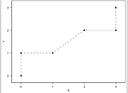
Discrete Distributions[15]. We take X vUniformf0; 1; 2; 3g and Y vBinomial 3;1₂ : It is easy to verify that

F_X1(p); F_Y1(p) = (0; 0) for 0 < p < 1 8; = (0; 1) for 1 8 < p < 2 8; = (1; 1) for 2 8 < p < 4 8; = (2; 2) for 4 8 < p < 6 8; = (3; 2) for 6 8 < p < 7 8; = (3; 3) for 7 8 < p < 1 8;

The support of (Xc_{; Y}c_{)is just these six points, and the connected support arises by}

simply connecting them consecutively with straight lines, the dotted lines in Figure 5:3. The straight line connecting (1; 1) and (2; 2) is not along, one of the axes. This happens because at level p = 1₂; both FX(y) and FY (y) have horizontal segments.

Note that any non-decreasing curve connecting (1; 1) and (2; 2) would have led to a feasible connected curve. These two points have probability 2₃; the other points 1₈:

3.3

Sums of comonotonic random variables

Notice that Sc is the sum of the components of the comonotonic counterpart (Xc

1; X2c; :::; Xnc)of a random vector (X1; X2; :::; Xn):

In this section, we will prove the fowllowing theorems which we give the approximation of the distribution function of S = X1 + X2+ ::: + Xn by the distribution function

of the comonotonic sum Sc _{is a prudent strategy in the sense that S}

cx Sc and

determining the marginal distribution functions of the terms in the sum.

In the next theorem we prove that the inverse disrtibution function of a sum of comonotonic random variables is simply the sum of the inverse distribution functions

of the marginal distributions.

Theorem 3.6 The inverse distribution F_Sc1( ) of a sum Sc of comonotonic

ran-dom variables (X1c; X2c; :::; Xnc) is given by

F_Sc1( )(p) = n X i=1 F_X1( ) i (p); 0 < p < 1; 0 1: (3.11)

Proof. Consider the random vector (X1; X2; :::; Xn) and its comonotonic

coun-terpart (Xc

1; X2c; :::; Xnc). Then Sc = X1c + X2c+ ::: + Xnc d

= g (U ) ; with U uniformly distributed on (0; 1) and with the function g de…ned by

g (u) = n X i=1 F_X1 i(u); 0 < u < 1:

It is clear that g is non-decreasing and left-continuous. Application of Theorem 2.24(a) leads to

F_Sc1(p) = F_{g(U )}1 (p) = g F_U1(p) = g(p); 0 < p < 1;

F_Sc1(p) = n X i=1 F_X1 i(p); 0 < p < 1:

Similarly, from Theorem 2.24(b), we …nd that

F_Sc1+(p) = n X i=1 F_X1+ i (p); 0 < p < 1:

Multiplying the last two equalities by and 1 respectively, and adding up, we …nd the desired result.

Note that Sc d= n X i=1 F_X1( ) i (U ): (3.12)

By the theorem above, we …nd that the connected support of Sc _{is given by}

n F_Sc1( )(p)j 0 < p < 1; 0 1 o ( _n X i=1 F_X1( ) i (p) j 0 < p < 1; 0 1 ) : This implies F_Sc1+(0) = n X i=1 F_X1+ i (0); (3.13) F_Sc1(1) = n X i=1 F_X1 i(1): (3.14)

Hence, The minimal value of the comonotonic sum equals the sum of the minimal values of each term. Similarly, the maximal value of the comonotonic sum equals the

sum of the maximal values of each term. The numberPn_i=1F_X1+

i (0), which is either

…nite or _{1 (if any the terms in the sum is 1), is the minimum possible value of} Sc_{, and} Pn

i=1F 1

Xi(1) is the maximum.

Also note that

F_Sc1+(1) = n X i=1 F_X1+ i (1) = +1; F_Sc1(0) = n X i=1 F_X1+ i (0) = 1:

For any (X1; X2; :::; Xn), we have that S = X1+ X2+ ::: + Xn Pn_i=1FXi1+(0) must

hold with probability 1. This implies

n X i=1 F_X1+ i (0) F 1+ S (0): (3.15) Similarly, we …nd F_S1(1) n X i=1 F_X1 i(1): (3.16)

This means that the sum S of the components of any random vector (X1; X2; :::; Xn)

has a support that is contained in the interval Pn_i=1F_X1+

i (0);

Pn i=1F

1

Xi(1) : The

minimal value of S is larger than or equal to the one of Sc, since by comonotonicity all terms of the latter are small simultaneously.

Given the inverse functions F_X1, the cdf of Sc _{= X}c

1+ X2c+ ::: + Xnc can be determined

FSc(x) = supfp 2 (0; 1) j F_Sc(x) pg (3.17) = sup p_{2 (0; 1) j FS}c1(p) x = sup ( p_{2 (0; 1) j} n X i=1 F_X1 i (p) x ) :

In the sequel, for any random variables X, the expression “FX increasing” should

always be interpreted as “FX is strictly increasing on FXi1+(0); F

1 Xi(1) ”.

Observe that for any random variable X, the following equivalences hold:

FX is strictly increasing , FX1is continuous on (0; 1) ; (3.18)

and also

FX is continuous , FX1 is strictly increasing on (0; 1) : (3.19)

Now assume that the marginal distribution functions FXi,i = 1; :::; n of the

comono-tonic random vector (Xc

1; X2c; :::; Xnc) are strictly increasing and continuous. Then

each inverse distribution function F_Xi1 is continuous on (0; 1), wich implies that F_Sc1

is continuous on (0; 1) because F_Sc1(p) =

Pn i=1F

1

Xi(p) holds for 0 < p < 1. This

in turn implies that FSc is strictly increasing on F_Sc1+(0); F_Sc1(1) . Further, by a

similar reasoning we …nd that FSc is continuous.

Hence, in case of strictly increasing and continuous marginals, for any F_Sc1+(0) <

equivalently,

n

X

i=1

F_Sc1(FSc(x)) = x; F_Sc1+(0) < x < F_Sc1(1): (3.20)

It su¢ ces thus to solve the latter equation to get FSc(x).

In the following theorem, we prove that also the stop-loss premiums of a sum of

comonotonic random variables can be obtained from the stop-loss premimiums of the terms.

Theorem 3.7 The stop-loss premiums of the sum Sc of the components of the co-monotonic random vector (Xc

1; X2c; :::; Xnc) are given by E (Sc d)₊ = n X i=1 E (Xi di)₊ ; FSc1+(0) < d < F_Sc1(1) ; (3.21)

with the di given by

di = F 1( d) Xi (FSc(d)); (i = 1; :::; n) (3.22) and d2 [0; 1] determined by F 1( d) Sc (FSc(d)) = d: (3.23)

Proof. _{Let d 2 FS}c1+(0); F_Sc1(1) , hence 0 < FSc(d) < 1:

As the connected support of Xc as de…ned in (3:9) is comonotonic, it can have at most one point of intersection with the hyperplane fx j x1+ ::: + xn= dg : This is

because the hyperplane contains no di¤erent points x and y such that x yor x y

Now we will prove that the vector d = (d1; d2; :::; dn) as de…ned above is the unique

point of this intersection. As 0 < FSc(d) < 1 must hold, we know from Section (2:6)

that there exists an d2 [0:1] that ful…ls condition (3:23). Also note that by Theorem

(3:6), we have that Pn_i=1di = d: Hence, the vector d with the di de…ned in (3:22)

and (3:23) is an element of both the connected support of Xc and the hyperplane fx j x1+ ::: + xn= dg :

We can conclude that d is the unique element of the intersection of the connected support and the hyperplane. Let x be an element of the connected support of Xc. Then the following equality holds:

(x1+ x2+ ::: + xn d)₊ (x1 d1)₊+ (x2 d2)₊+ ::: + (xn dn)₊:

This is because x and d are both elements of the connected support of Xc, and hence,

if there exists any j such that xj > dj holds, then we also have xk dk for all k, and

the left hand side equals the right hand side becausePn_i=1di = d:On the other hand,

when all xj dj, obviously the left hand side is 0 as well.

Now replacing constants by the corresponding random variables in the equality above and taking expectations, we …nd (3:21).

Note that we also …nd that

E (Sc d)₊ = n X i=1 E [Xi] d; if d FSc1+(0) (3.24) and E (Sc d)₊ = 0; if d F_Sc1(1): (3.25)

So from (3:13), (3:14), (3:24), (3:25) and Theorem (3:7) we can conclude that for any real d, there exist diwith

Pn

i=1di = d, such that E (Sc d)+ =

Pn

i=1E (Xi di)+

holds.

The expression for the stop-loss premiums of a comonotonic sum Sc can also be written in terms of the usual inverse distribution functions. Indeed, for any retention d_{2 FS}c1+(0); F_Sc1(1) , we have E Xi F 1( d) Xi (FSc(d)) ₊ = Eh Xi FXi1(FSc(d)) + i F 1( d) Xi (FSc(d)) F 1 Xi (FSc(d)) (1 FSc(d))

Summing over i, and taking into account the de…nition of d, we …nd the

expres-sion derived in Dhaene, Wang, Young & Goovaerts (2000), where the random vari-ables were assumed to be non-negative. This expression holds for any retention d_{2 FS}c1+(0); F_Sc1(1) : E (Sc d)₊ = n X i=1 Eh Xi FXi1(FSc(d)) + i (3.26) d F_Sc1(FSc(d)) (1 F_Sc(d)) :

In case the marginal cdf’s FXi are strictly increasing, (3:26) reduces to

E (Sc d)₊ = n X i=1 Eh Xi FXi1(FSc(d)) + i ; d_{2 FS}c1+(0); F_Sc1(1) : (3.27)

From Theorem (3:7), we can conclude that ant stop-loss premium of a sum of co-monotonic random variables can be written as the sum of stop-loss premiums for

the individual random variables involved. The theorem provided an algorithm for directly computing stop-loss premiums of sums of comonotonic random variables,

without having to compute the stop-loss premium with retention d, we only need to know FSc(d), which can be computed directly from (3:17).

Application of the relation E (X d)_{+ = E (d} X)_{+ + E [X]} d for Sc _{and the}

Xi in relation (3:21) leads to the following expression for the lower tails of a sum of

comonotonic random variables:

E (d Sc)₊ =

n

X

i=1

E [(di Xi)] ; FSc1+(0) < d < F_Sc1(1); (3.28)

with the di as de…ned in (3:22) and (3:23).

The comonotonic upper bound for Pn_i=1Xi

Theorem 3.8 ([15]) For any vector (X1; X2; :::; Xn) we have

X1+ X2+ ::: + Xn cx X1c+ X c

2 + ::: + X c

n: (3.29)

3.4

The New Results

The main results of this work are the following theorem, and proposition.

3.4.1

Convex bounds and the comonotonic upper bound for

S

In risk theory and …nance, one is often interested in distribution of the sums

individual risks of a portfolio X: In this subsection we give a short overview of these stochastic ordering results. For proofs and more details on the presented results, we refer to the overview paper of Dhaene et al.[9] and Zeghdoudi and Remita [56].

Theorem 3.9 (M.Bouhadjar et al.) We note that:

~

SN = ~X1f (Y1) + ~X2f (Y2) + ::: + ~Xnf (Yn) (3.30)

For any random vector X = (X1; :::; Xn) and f (Yi); i = 1; :::; n we have

SN cxS~N: (3.31)

Proof_{. It is su¢ ces to prove stop-loss order because E (S}N) = E ~SN : Hence,

we have to prove that

E[(SN d)+] E[( ~SN d)+]

The following holds for all (X1f (Y1); X2f (Y2); :::; Xnf (Yn))when d1+ d2+ ::: + dn= d

(X1f (Y1) + X2f (Y2) + ::: + Xnf (Yn) d)₊

= (X1f (Y1) d1+ X2f (Y2) d2+ ::: + Xnf (Yn) dn)+

(X1f (Y1) d1)++ (X2f (Y2) d2)++ ::: + (Xnf (Yn) dn)_{+ +}

= (X1f (Y1) d1)₊+ (X2f (Y2) d2)₊+ ::: + (Xnf (Yn) dn)₊

Now taking expectations, we get that

E (X1f (Y1) + X2f (Y2) + ::: + Xnf (Yn) d)₊ n

X

i=1

According to [15] we have E[( ~SN d)+] = n X i=1 E (Xif (Yi) di)+ Then, SN cxS~N:

Proposition 3.10 For any random vector X = (X1; :::; Xn), any random variable

and for U v Uniform(0; 1), which is assumed to be a function of X and for f (Yi) 1; i = 1; :::; n, we have, (a) S cxSN (3.32) (b) ~ S cxS~N (3.33) (c) n X j=1 E [Xi j ] cxSN (3.34) (d) n X j=1 EhX~i j i cxS~N (3.35) Proof.

(a) We have f (Yi) 1; i = 1; :::; n and we used property 10 and 6, we obtain

thus

S cx SN:

(b) We will omit the proof here because the idea is very similar to the proof in (a). (c) According to Dhaene et al.[9] we have,

n

P

j=1E [X

i j ] cx S and (a), we deduce

that

n

X

j=1

E [Xi j ] cxSN:

(d) According to Zeghdoudi and Remita [56] we have

n P j=1E h ~ Xi j i cx S, using~

property 12 and (b), we obtain

n X j=1 EhX~i j i cxS~N:

In addition, if f (Yi) 1; i = 1; :::; n;we can check easily that

Chapter 4

Policy Limits and Deductibles

If the sum of policy limits(deductible) is …xed, then Xi st Xj ) li lj and

d_i d_j when ( X1; X2; :::; Xn) is comonotonic, where li : optimal policy limit and

d_i : optimal deductible allocated to i-th risk.

In this chapter we present the problem of the optimal allocation of policy limits and deductibles. For make the new general model analytically tractable, we will make the following assumptions :

1. the policyholder is risk-averse, and therefore the utility function is increasing and concave;

2. the random vector X = (X1; :::; Xn), which represents the loss severities, and

random vector Y = (Y1; :::; Yn), which represents the time of occurrence of losses, are

independent; moreover, Y1; :::; Yn are mutually independent;

4.1

Policy limits with unknown dependent

struc-tures

The …rst problem to be considered is to maximize the expected utility of wealth:

max min I2An(l)X2RE " u w n X i=1 Xi (Xi^ li)₊ f (Yi) !# (4.1)

where u and w are the utility function (increasing and concave), the wealth (after premium) respectively and ~u is an increasing convex function. The problem is

equi-valent to min max l2An(l)X2RE " ~ u n X i=1 (Xi li)₊f (Yi) !# (4.2)

Lemma 4.1 (B) If ( ~X1; :::; ~Xn)2 R comonotonic, then

E " ~ u n X i=1 (Xi li)+f (Yi) !# E " ~ u n X i=1 ~ Xi li +f (Yi) !# (4.3)

for any (l1; :::; ln)2 An(l) and (X1; :::; Xn)2 R independent of Y.

Proof. Let ~X = ( ~X1; :::; ~Xn) 2 R be comonotonic and independent of Y. For

any …xed constants y1; :::; yn, Theorem (3:4) implies that

~ X1 l1 +f (y1); :::; ~ Xn ln +f (yn)

is still comonotonic. Therefore, by Theorem (3:8) and Theorem (3:9), we have

n X i=1 (Xi li)₊f (yi) cx n X i=1 ~ Xi li +f (yi)

because ~u is increasing and convex. Then by the independence of X and Y, E " ~ u n X i=1 (Xi li)+f (Yi) !# = E " E ( ~ u n X i=1 (Xi li)+f (Yi) ! j Y1; :::; Yn )# E " E ( ~ u n X i=1 ~ Xi li +f (Yi) ! j Y1; :::; Yn )# = E " ~ u n X i=1 ~ Xi li +f (Yi) !# : and hence E " ~ u n X i=1 (Xi li)₊f (yi) !# E " ~ u n X i=1 ~ Xi li + f (yi) !#

Now, the initial problem becomes Problem L0 _{: min}

l2An(l)E ~u

Pn

i=1(Xi li)+f (Yi)

Proposition 4.2 Let l = (l1; :::; ln) be the solution to Problem L0, then

Yi lr Yj; Xi st Xj ) li lj: (4.4)

Proof. Assume that li lj. Since x ! f(Yi)is decreasing , by property 13

Yi lr Yj ) f(Yi) lr f (Yj)

Since (Xi; Xj)is comonotonic and Xi st Xj , Xi(!) Xj(!) for any ! 2 . By the

independence of X and Y, we can hereafter …x an outcome of (X1; :::; Xi; :::; Xj; :::; Xn)

as (x1; :::; xi; :::; xj; :::; xn)with xi xj. As g(x; I) =

Pn

i=1(xi li)+ is an AI

decreasing in x, then by Lemma (2:12)

((xi li)+; (xj lj)+) ((xi lj)+; (xj li)+)

Since wehave (xi lj)+ (xj li)+, then by property 14 we have

(xi li)+f (Yi) + (xj lj)+f (Yj) icx(xi lj)+f (Yi) + (xj li)+f (Yj):

Morever, for the increasing convex function ~u,

E " ~ u( xi li)+f (Yi) + (xj lj)+f (Yj) + X k6=i;j (xk lk)+f (Yk) !# E " ~ u (xi lj)+f (Yi) + (xj li)+f (Yj) + X k6=i;j (xk lk)+f (Yk) !#

By taking expectations conditional on X, we obtain

E " ~ u (Xi li)+f (Yi) + (Xj lj)+f (Yj) + X k6=i;j (Xk lk)+f (Yk) !# E " ~ u (Xi lj)+f (Yi) + (Xj li)+f (Yj) + X k6=i;j (Xk lk)+f (Yk) !#

The result follows.

4.2

Policy deductibles with unknown dependent

structures

The same thing is made that the of policy limits, we consider the problem of the optimal allocation of deductibles :

max min d2An(d)X2RE " u w n X i=1 Xi (Xi di)+ f (Yi) !# (4.5) which we have min max d2An(d)X2RE " ~ u n X i=1 (Xi^ di)+f (Yi) !# (4.6)

Lemma 4.3 If ( ~X1; :::; ~Xn)2 R is comonotonic and independent of Y, then

E " ~ u n X i=1 (Xi^ di)+f (Yi) !# E " ~ u n X i=1 ~ Xi^ di +f (Yi) !# (4.7)

for any (d1; :::; dn)2 An(d) and (X1; :::; Xn)2 R independent of Y.

The proof is similar to the proof of Lemma B. From the above lemma, our problem becomes Problem D0 _{: min}

d2An(d)E ~u

Pn

i=1(Xi^ di)+f (Yi)

Proposition 4.4 Let d = (d₁; :::; d_n) be the solution to Problem D0_{, then}

Yi lr Yj; Xi st Xj ) di dj: (4.8)

Proof. Assume that di dj:As in the proof of Proposition (4:2), we have

Yi lr Yj ) f(Yi) lrf (Yj);

And we can …x an outcome of (X1; :::; Xi; :::; Xj; :::; Xn) as (x1; :::; xi; :::; xj; :::; xn)

with xi xj. As g(x; d) =

Pn

function (x; d) ! x ^ d is increasing both in x and d, then by Lemma (2:11),

((xi^ di); (xj^ dj)) ((xi^ dj); (xj ^ di)):

Since we also have (xi^ dj) (xj ^ di), then by property 14 we have

(xi^ di)f (Yi) + (xj ^ dj)f (Yj) icx (xi^ dj)f (Yi) + (xj ^ di)f (Yj)

By independence convolution, we have

(xi^ di)f (Yi) + (xj^ dj)f (Yj) + X k6=i;j (xk^ dk)+f (Yk) icx(xi^ dj)f (Yi) + (xj ^ di)f (Yj) + X k6=i;j (xk^ dk)+f (Yk)

Morever, for the increasing convex function ~u,

E " ~ u (xi^ di)f (Yi) + (xj ^ dj)f (Yj) + X k6=i;j (xk^ dk)+f (Yk) !# E " ~ u (xi^ dj)f (Yi) + (xj^ di)f (Yj) + X k6=i;j (xk^ dk)+f (Yk) !#

With a same manner we …nd the result on X.

4.3

Some examples and Application

In this section we will describe several examples that show how distribution func-tion of the sum of random variables can be approximated by convex order of random

variable (see Rüschendorf [48]) for lower convex order of random variables and com-parison of two families of copulas.

4.3.1

Lower Bound Approximations of the Distribution Sum

of Random Variables with Convex Ordering

Example 4.5 (Approximation of distribution sum of two independent standard

nor-mal random variables)[22]

Suppose X and Y be independent N (0; 1) random variables. We want to derive

lower bounds for S = X + Y . In this case we know the exact distribution of S, i.e S v N(0; 2). Let us see how lower bound approximation works in this case. Let Z = X + aY for some real a. Then Z v N(0; 1 + a2_{). Therefore, for some choices of}

a, we get the following distribution for the lower bound for S :

a = 0gives N (0; 1) cxS = X + Y v N(0; 2)

a = 1gives N (0; 2) cxS = X + Y v N(0; 2)

a = 1 gives N (0; 2) cxS = X + Y v N(0; 2)

Thus in this case best lower bound is obtained for a = 1 which is the exact distribution. The variance of the lower bound can be seen to have a maximum at a = 1 and a minimum at a = 1.

Example 4.6 [15]

As a theoretical example, consider an insurance portfolio consisting of n risks. The payments to be made by the insurer are described by a random vector (X1 +

X2+ ::: + Xn), where Xi is the claim amount of policy i during the insurance period.

We assume that all payments have to be done at the end of the insurance period [0; 1]. In a deterministic …nancialsetting, the present value at time 0 of the aggregate

claims X1+ X2+ ::: + Xn to be paid by the insurer at time 1 is determined by

S = (X1+ X2+ ::: + Xn)

where = (1 + r) 1 _{is the deterministic discount factor and r is the technical interest}

rate. This will be chosen in a conservative way (i.e.su¢ ciently low), if the insurer doesn’t want to underestimate his future obligations. To demonstrate the e¤ect of introducing random interest on insurance business, we look at the following special

case. Assume all risks Xi to be non-negative, independent and identically

distrib-uted,and let X = Xd i, where the symbol d

=is used to indicate equality in distribution. The average payment S

n has mean and variance

E S_n = E(X); V S_n =

2

n V(X)

The stability necessary for both insureds and insurer is maintained by the Law of Large Numbers, provided that n is indeed ‘large’and that the risks are mutually

independent and rather well-behaved, not describing for instance risks of catastrophic nature for which the variance might be very large or even in…nite.