HAL Id: hal-01758912
https://hal.archives-ouvertes.fr/hal-01758912v2
Submitted on 7 Apr 2018
HAL is a multi-disciplinary open access archive for the deposit and dissemination of sci-entific research documents, whether they are pub-lished or not. The documents may come from teaching and research institutions in France or
L’archive ouverte pluridisciplinaire HAL, est destinée au dépôt et à la diffusion de documents scientifiques de niveau recherche, publiés ou non, émanant des établissements d’enseignement et de recherche français ou étrangers, des laboratoires
Dynamic Load Balancing with Tokens
Céline Comte
To cite this version:
Céline Comte. Dynamic Load Balancing with Tokens. IFIP Networking, May 2018, Zurich, Switzer-land. �10.23919/IFIPNetworking.2018.8697018�. �hal-01758912v2�
Dynamic Load Balancing with Tokens
∗
C´
eline Comte
Nokia Bell Labs and T´
el´
ecom ParisTech, University Paris-Saclay, France
[email protected]
April 7, 2018
Efficiently exploiting the resources of data centers is a complex task that requires efficient and reliable load balancing and resource allocation algorithms. The former are in charge of assigning jobs to servers upon their arrival in the system, while the latter are responsible for sharing server resources between their assigned jobs. These algorithms should take account of various constraints, such as data locality, that re-strict the feasible job assignments. In this paper, we propose a token-based mecha-nism that efficiently balances load between servers without requiring any knowledge on job arrival rates and server capacities. Assuming a balanced fair sharing of the server resources, we show that the resulting dynamic load balancing is insensitive to the job size distribution. Its performance is compared to that obtained under the best static load balancing and in an ideal system that would constantly optimize the resource utilization.
1 Introduction
The success of cloud services encourages operators to scale out their data centers and opti-mize the resource utilization. The current trend consists in virtualizing applications instead of running them on dedicated physical resources [2]. Each server may then process several applications in parallel and each application may be distributed among several servers. Better understanding the dynamics of such server pools is a prerequisite for developing load balancing and resource allocation policies that fully exploit this new degree of flexibility.
Some recent works have tackled this problem from the point of view of queueing theory [1, 15, 9, 4]. Their common feature is the adoption of a bipartite graph that translates practical constraints such as data locality into compatibility relations between jobs and servers. These models apply in various systems such as computer clusters, where the shared resource is the CPU [9, 4], and content delivery networks, where the shared resource is the server upload band-width [15]. However, these pool models do not consider simultaneously the impact of complex load balancing and resource allocation policies. The model of [1] lays emphasis on dynamic load balancing, assuming neither server multitasking nor job parallelism. The bipartite graph describes the initial compatibilities of incoming jobs, each of them being eventually assigned to a
∗
c
IFIP, 2018. This is the author’s version of the work. It is posted here by permission of IFIP for your personal use. Not for redistribution. The definitive version will be published in IFIP NETWORKING 2018 proceedings.
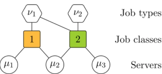
µ1 µ2 µ3 1 2 ν1 ν2 Servers Job classes Job types
Figure 1: A compatibility graph between types, classes and servers. Two consecutive servers can be pooled to process jobs in parallel. Thus there are two classes, one for servers 1 and 2 and another for servers 2 and 3. Type-1 jobs can be assigned to any class, while type-2 jobs can only be assigned to the latter. This restriction may result from data locality constraints for instance.
single server. On the other hand, [9, 15, 4] focus on the problem of resource allocation, assuming a static load balancing that assigns incoming jobs to classes at random, independently of the system state. The class of a job in the system identifies the set of servers that can be pooled to process it in parallel. The corresponding bipartite graph, connecting classes to servers, restricts the set of feasible resource allocations.
In this paper, we introduce a tripartite graph that explicitly differentiates the compatibilities of an incoming job from its actual assignment by the load balancer. This new model allows us to study the joint effect of load balancing and resource allocation. A toy example is shown in Figure 1. Each incoming job has a type that defines its compatibilities; these may reflect its parallelization degree or locality constraints, for instance. Depending on the system state, the load balancer matches the job with a compatible class that subsequently determines its assigned servers. The upper part of our graph, which puts constraints on load balancing, corresponds to the bipartite graph of [1]; the lower part, which restricts the resource allocation, corresponds to the bipartite graph of [9, 15, 4].
We use this new framework to study load balancing and resource allocation policies that are insensitive, in the sense that they make the system performance independent of fine-grained traffic characteristics. This property is highly desirable as it allows service providers to di-mension their infrastructure based on average traffic predictions only. It has been extensively studied in the queueing literature [6, 7, 5, 15]. In particular, insensitive load balancing policies were introduced in [5] in a generic queueing model, assuming an arbitrary insensitive allocation of the resources. These load balancing policies were defined as a generalization of the static load balancing described above, where the assignment probabilities of jobs to classes depend on both the job type and the system state, and are chosen to preserve insensitivity.
Our main contribution is an algorithm based on tokens that enforces such an insensitive load balancing without performing randomized assignments. More precisely, this is a deterministic implementation of an insensitive load balancing that adapts dynamically to the system state, under an arbitrary compatibility graph. The principle is as follows. The assignments are regulated through a bucket containing a fixed number of tokens of each class. An incoming job seizes the longest available token among those that identify a compatible class, and is blocked if it does not find any. The rationale behind this algorithm is to use the release order of tokens as an information on the relative load of their servers: a token that has been available for a long time without being seized is likely to identify a server set that is less loaded than others. As we will see, our algorithm mirrors the first-come, first-served (FCFS) service discipline proposed in [4] to implement balanced fairness, which was defined in [7] as the most efficient insensitive resource allocation.
The closest existing algorithm we know is assign longest idle server (ALIS), introduced in reference [1] cited above. This work focuses on server pools without job parallel processing nor server multitasking. Hence, ALIS can be seen as a special case of our algorithm where each class identifies a server with a single token. The algorithm we propose is also related to the blocking version of Join-Idle-Queue [13] studied in [16]. More precisely, we could easily generalize our algorithm to server pools with several load balancers, each with their own bucket. The corresponding queueing model, still tractable using known results on networks of quasi-reversible queues [11], extends that of [16].
Organization of the paper Section 2 recalls known facts about resource allocation in server pools. We describe a standard pool model based on a bipartite compatibility graph and explain how to apply balanced fairness in this model. Section 3 contains our main contributions. We describe our pool model based on a tripartite graph and introduce a new token-based insensitive load balancing mechanism. Numerical results are presented in Section 4.
2 Resource allocation
We first recall the model considered in [9, 15, 4] to study the problem of resource allocation in server pools. This model will be extended in Section 3 to integrate dynamic load balancing.
2.1 Model
We consider a pool of S servers. There are N job classes and we let I = {1, . . . , N } denote the set of class indices. For now, each incoming job is assigned to a compatible class at random, independently of the system state. For each i ∈ I, the resulting arrival process of jobs assigned to class i is assumed to be Poisson with a rate λi> 0 that may depend on the job arrival rates,
compatibilities and assignment probabilities. The number of jobs of class i in the system is limited by `i, for each i ∈ I, so that a new job is blocked if its assigned class is already full.
Job sizes are independent and exponentially distributed with unit mean. Each job leaves the system immediately after service completion.
The class of a job defines the set of servers that can be pooled to process it. Specifically, for each i ∈ I, a job of class i can be served in parallel by any subset of servers within the non-empty set Si ⊂ {1, . . . , S}. This defines a bipartite compatibility graph between classes
and servers, where there is an edge between a class and a server if the jobs of this class can be processed by this server. Figure 2 shows a toy example.
µ1 µ2 µ3
λ1 λ2
Servers Job classes
Figure 2: A compatibility graph between classes and servers. Servers 1 and 3 are dedicated, while server 2 can serve both classes. The server sets associated with classes 1 and 2 are S1 = {1, 2} and S2 = {2, 3}, respectively.
When a job is in service on several servers, its service rate is the sum of the rates allocated by each server to this job. For each s = 1, . . . , S, the capacity of server s is denoted by µs> 0.
We can then define a function µ on the power set of I as follows: for each A ⊂ I,
µ(A) = X
s∈S
i∈ASi
µs
denotes the aggregate capacity of the servers that can process at least one class in A, i.e., the maximum rate at which jobs of these classes can be served. µ is a submodular, non-decreasing set function [8]. It is said to be normalized because µ(∅) = 0.
2.2 Balanced fairness
We first recall the definition of balanced fairness [7], which was initially applied to server pools in [15]. Like processor sharing (PS) policy, balanced fairness assumes that the capacity of each server can be divided continuously between its jobs. It is further assumed that the resource allocation only depends on the number of jobs of each class in the system; in particular, all jobs of the same class receive service at the same rate.
The system state is described by the vector x = (xi : i ∈ I) of numbers of jobs of each class
in the system. The state space is X = {x ∈ NN : x ≤ `}, where ` = (`i : i ∈ I) is the vector
of per-class constraints and the comparison ≤ is taken componentwise. For each i ∈ I, we let φi(x) denote the total service rate allocated to class-i jobs in state x. It is assumed to be
nonzero if and only if xi> 0, in which case each job of class i receives service at rate φi(x)/xi.
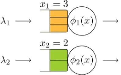
Queueing model Since all jobs of the same class receive service at the same rate, we can describe the evolution of the system with a network of N PS queues with state-dependent service capacities. For each i ∈ I, queue i contains jobs of class i; the arrival rate at this queue is λi and its service capacity is φi(x) when the network state is x. An example is shown in
Figure 3 for the configuration of Figure 2.
φ1(x) x1= 3 λ1 φ2(x) x2= 2 λ2
Figure 3: An open Whittle network of N = 2 queues associated with the server pool of Figure 2.
Capacity set The compatibilities between classes and servers restrict the set of feasible resource allocations. Specifically, the vector (φi(x) : i ∈ I) of per-class service rates belongs to the
following capacity set in any state x ∈ X :
Σ = ( φ ∈ RN+ : X i∈A φi≤ µ(A), ∀A ⊂ I ) .
Balance function It was shown in [6] that the resource allocation is insensitive if and only if there is a balance function Φ defined on X such that Φ(0) = 1 and
φi(x) =
Φ(x − ei)
Φ(x) , ∀x ∈ X , ∀i ∈ I(x), (1)
where ei is the N -dimensional vector with 1 in component i and 0 elsewhere and I(x) = {i ∈
I : xi > 0} is the set of active classes in state x. Under this condition, the network of PS queues defined above is a Whittle network [14]. The insensitive resource allocations that respect the capacity constraints of the system are characterized by a balance function Φ such that, for all x ∈ X \ {0}, Φ(x) ≥ 1 µ(A) X i∈A Φ(x − ei), ∀A ⊂ I(x), A 6= ∅.
Recursively maximizing the overall service rate in the system is then equivalent to minimizing Φ by choosing Φ(x) = max A⊂I(x), A6=∅ 1 µ(A) X i∈A Φ(x − ei) ! , ∀x ∈ X \ {0}.
The resource allocation defined by this balance function is called balanced fairness.
It was shown in [15] that balanced fairness is Pareto-efficient in polymatroid capacity sets, meaning that the total service rate P
i∈I(x)φi(x) is always equal to the aggregate capacity
µ(I(x)) of the servers that can process at least one active class. By (1), this is equivalent to
Φ(x) = 1
µ(I(x)) X
i∈I(x)
Φ(x − ei), ∀x ∈ X \ {0}. (2)
Stationary distribution The Markov process defined by the system state x is reversible, with stationary distribution
π(x) = π(0)Φ(x)Y
i∈I
λixi, ∀x ∈ X . (3)
By insensitivity, the system state has the same stationary distribution if the jobs sizes within each class are only i.i.d., as long as the traffic intensity of class i (defined as the average quantity of work brought by jobs of this class per unit of time) is λi, for each i ∈ I. A proof of this result
is given in [6] for Cox distributions, which form a dense subset within the set of distributions of nonnegative random variables.
2.3 Job scheduling
We now describe the sequential implementation of balanced fairness that was proposed in [4]. This will lay the foundations for the results of Section 3.
We still assume that a job can be distributed among several servers, but we relax the as-sumption that servers can process several jobs at the same time. Instead, each server processes its jobs sequentially in FCFS order. When a job arrives, it enters in service on every idle server within its assignment, if any, so that its service rate is the sum of the capacities of these servers. When the service of a job is complete, it leaves the system immediately and its servers are re-allocated to the first job they can serve in the queue. Note that this sequential implementation also makes sense in a model where jobs are replicated over several servers instead of being pro-cessed in parallel. For more details, we refer the reader to [9] where the model with redundant requests was introduced.
Since the arrival order of jobs impacts the rate allocation, we need to detail the system state. We consider the sequence c = (c1, . . . , cn) ∈ I∗, where n is the number of jobs in the system
and cp is the class of the p-th oldest job, for each p = 1, . . . , n. ∅ denotes the empty state, with
n = 0. The vector of numbers of jobs of each class in the system, corresponding to the state introduced in §2.2, is denoted by |c| = (|c|i : i ∈ I) ∈ X . It does not define a Markov process in
general. We let I(c) = I(|c|) denote the set of active classes in state c. The state space of this detailed system state is C = {c ∈ I∗ : |c| ≤ `}.
Queueing model Each job is in service on all the servers that were assigned this job but not those that arrived earlier. For each p = 1, . . . , n, the service rate of the job in position p is thus given by
X
s∈Scp\Sp−1q=1Scq
µs= µ(I(c1, . . . , cp)) − µ(I(c1, . . . , cp−1)),
with the convention that (c1, . . . , cp−1) = ∅ if p = 1. The service rate of a job is independent of
the jobs arrived later in the system. Additionally, the total service rate µ(I(c)) is independent of the arrival order of jobs. The corresponding queueing model is an order-independent (OI) queue [3, 12]. An example is shown in Figure 4 for the configuration of Figure 2.
2 1 2 1 1 c = (1, 1, 2, 1, 2)
µ(I(c)) λ1
λ2
Figure 4: An OI queue with N = 2 job classes associated with the server pool of Figure 2. The job of class 1 at the head of the queue is in service on servers 1 and 2. The third job, of class 2, is in service on server 3. Aggregating the state c yields the state x of the Whittle network of Figure 3.
Stationary distribution The Markov process defined by the system state c is irreducible. The results of [12] show that this process is quasi-reversible, with stationary distribution
π(c) = π(∅)Φ(c)Y
i∈I
λi|c|i, ∀c ∈ C, (4)
where Φ is defined recursively on C by Φ(∅) = 1 and
Φ(c) = 1
µ(I(c))Φ(c1, . . . , cn−1), ∀c ∈ C \ {∅}. (5)
We now go back to the aggregate state x giving the number of jobs of each class in the system. With a slight abuse of notation, we let
π(x) = X
c:|c|=x
π(c) and Φ(x) = X
c:|c|=x
Φ(c), ∀x ∈ X .
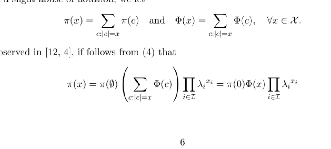
As observed in [12, 4], if follows from (4) that
π(x) = π(∅) X c:|c|=x Φ(c) Y i∈I λixi = π(0)Φ(x) Y i∈I λixi
in any state x. Using (5), we can show that Φ satisfies (2) with the initial condition Φ(0) = Φ(∅) = 1. Hence, the stationary distribution of the aggregate system state x is exactly that obtained in §2.2 under balanced fairness.
It was also shown in [4] that the average per-class resource allocation resulting from FCFS service discipline is balanced fairness. In other words, we have
φi(x) =
X
c:|c|=x
π(c)
π(x)µi(c), ∀x ∈ X , ∀i ∈ I(x),
where φi(x) is the total service rate allocated to class-i jobs in state x under balanced fairness,
given by (1), and µi(c) denotes the service rate received by the first job of class i in state c
under FCFS service discipline: µi(c) = n X p=1 cp=i (µ(I(c1, . . . , cp)) − µ(I(c1, . . . , cp−1))).
Observe that, by (3) and (4), the rate equality simplifies to φi(x) =
X
c:|c|=x
Φ(c)
Φ(x)µi(c), ∀x ∈ X , ∀i ∈ I(x). (6)
We will use this last equality later.
As it is, the FCFS service discipline is very sensitive to the job size distribution. [4] mitigates this sensitivity by frequently interrupting jobs and moving them to the end of the queue, in the same way as round-robin scheduling algorithm in the single-server case. In the queueing model, these interruptions and resumptions are represented approximately by random routing, which leaves the stationary distribution unchanged by quasi-reversibility [11, 14]. If the inter-ruptions are frequent enough, then all jobs of a class tend to receive the same service rate on average, which is that obtained under balanced fairness. In particular, performance becomes approximately insensitive to the job size distribution within each class.
3 Load balancing
The previous section has considered the problem of resource sharing. We now focus on dynamic load balancing, using the fact that each job may be a priori compatible with several classes and assigned to one of them upon arrival. We first extend the model of §2.1 to add this new degree of flexibility.
3.1 Model
We again consider a pool of S servers. There are N job classes and we let I = {1, . . . , N } denote the set of class indices. The compatibilities between job classes and servers are described by a bipartite graph, as explained in §2.1. Additionally, we assume that the arrivals are divided into K types, so that the jobs of each type enter the system according to an independent Poisson process. Job sizes are independent and exponentially distributed with unit mean. Each job leaves the system immediately after service completion.
The type of a job defines the set of classes it can be assigned to. This assignment is performed instantaneously upon the job arrival, according to some decision rule that will be detailed later.
For each i ∈ I, we let Ki ⊂ {1, . . . , K} denote the non-empty set of job types that can be
assigned to class i. This defines a bipartite compatibility graph between types and classes, where there is an edge between a type and a class if the jobs of this type can be assigned to this class. Overall, the compatibilities are described by a tripartite graph between types, classes, and servers. Figure 1 shows a toy example.
For each k = 1, . . . , K, the arrival rate of type-k jobs in the system is denoted by νk> 0. We
can then define a function ν on the power set of I as follows: for each A ⊂ I,
ν(A) = X
k∈S
i∈AKi
νk
denotes the aggregate arrival rate of the types that can be assigned to at least one class in A. ν satisfies the submodularity, monotonicity and normalization properties satisfied by the function µ of §2.1.
3.2 Randomized load balancing
We now express the insensitive load balancing of [5] in our new server pool model. This extends the static load balancing considered earlier. Incoming jobs are assigned to classes at random, and the assignment probabilities depend not only on the job type but also on the system state. As in §2.2, we assume that the capacity of each server can be divided continuously between its jobs. The resources are allocated by applying balanced fairness in the capacity set defined by the bipartite compatibility graph between job classes and servers.
Open queueing model We first recall the queueing model considered in [5] to describe the randomized load balancing. As in §2.2, jobs are gathered by class in PS queues with state-dependent service capacities given by (1). Hence, the type of a job is forgotten once it is assigned to a class.
Similarly, we record the job arrivals depending on the class they are assigned to, regardless of their type before the assignment. The Poisson arrival assumption ensures that, given the system state, the time before the next arrival at each class is exponentially distributed and independent of the arrivals at other classes. The rates of these arrivals result from the load balancing. We write them as functions of the vector y = ` − x of numbers of available positions at each class. Specifically, λi(y) denotes the arrival rate of jobs assigned to class i when there
are yj available positions in class j, for each j ∈ I.
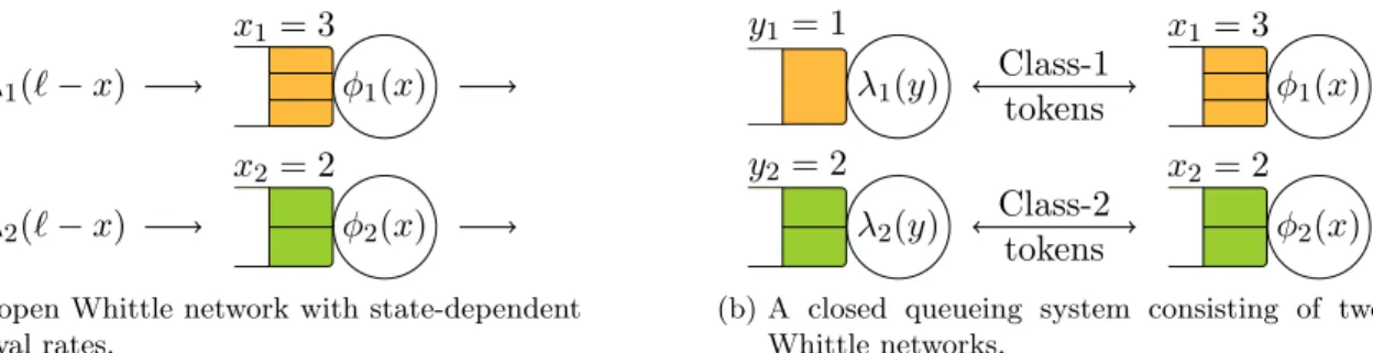
φ1(x) x1 = 3 φ2(x) x2 = 2 λ1(` − x) λ2(` − x)
(a) An open Whittle network with state-dependent arrival rates. λ1(y) y1 = 1 λ2(y) y2 = 2 φ1(x) x1 = 3 φ2(x) x2 = 2 Class-1 tokens Class-2 tokens
(b) A closed queueing system consisting of two Whittle networks.
Figure 5: Alternative representations of a Whittle network associated with the server pool of Figure 1. At most `1 = `2= 4 jobs can be assigned to each class.
The system can thus be modeled by a network of N PS queues with state-dependent arrival rates, as shown in Figure 5a.
Closed queueing model We introduce a second queueing model that describes the system dynamics differently. It will later simplify the study of the insensitive load balancing by drawing a parallel with the resource allocation of §2.2.
Our alternative model stems from the following observation: since we impose limits on the number of jobs of each class, we can indifferently assume that the arrivals are limited by the intermediary of buckets containing tokens. Specifically, for each i ∈ I, the assignments to class i are controlled through a bucket filled with `i tokens. A job that is assigned to class i removes
a token from this bucket and holds it until its service is complete. The assignments to a class are suspended when the bucket of this class is empty, and they are resumed when a token of this class is released.
Each token is either held by a job in service or waiting to be seized by an incoming job. We consider a closed queueing model that reflects this alternation: a first network of N queues contains tokens held by jobs in service, as before, and a second network of N queues contains available tokens. For each i ∈ I, a token of class i alternates between the queues indexed by i in the two networks. This is illustrated in Figure 5b.
The state of the network containing tokens held by jobs in service is x. The queues in this network apply PS service discipline and their service capacities are given by (1). The state of the network containing available tokens is y = ` − x. For each i ∈ I, the service of a token at queue i in this network is triggered by the arrival of a job assigned to class i. The service capacity of this queue is thus equal to λi(y) in state y. Since all tokens of the same class are
exchangeable, we can assume indifferently that we pick one of them at random, so that the service discipline of the queue is PS.
Capacity set The compatibilities between job types and classes restrict the set of feasible load balancings. Specifically, the vector (λi(y) : i ∈ I) of per-class arrival rates belongs to the
following capacity set in any state y ∈ X :
Γ = ( λ ∈ RN+ : X i∈A λi ≤ ν(A), ∀A ⊂ I ) .
The properties satisfied by ν guarantee that Γ is a polymatroid.
Balance function Our token-based reformulation allows us to interpret dynamic load balancing as a problem of resource allocation in the network of queues containing available tokens. This will allow us to apply the results of §2.2.
It was shown in [5] that the load balancing is insensitive if and only if there is a balance function Λ defined on X such that Λ(0) = 1, and
λi(y) =
Λ(y − ei)
Λ(y) , ∀y ∈ X , ∀i ∈ I(y). (7)
Under this condition, the network of PS queues containing available tokens is a Whittle network. The Pareto-efficiency of balanced fairness in polymatroid capacity sets can be understood as follows in terms of load balancing. We consider the balance function Λ defined recursively on
X by Λ(0) = 1 and Λ(y) = 1 ν(I(y)) X i∈I(y) Λ(y − ei), ∀y ∈ X \ {0}. (8)
Then Λ defines a load balancing that belongs to the capacity set Γ in each state y. By (7), this load balancing satisfies
X
i∈I(y)
λi(y) = ν(I(y)), ∀y ∈ X ,
meaning that an incoming job is accepted whenever it is compatible with at least one available token.
Stationary distribution The Markov process defined by the system state x is reversible, with stationary distribution
π(x) = 1
GΦ(x)Λ(` − x), ∀x ∈ X , (9)
where G is a normalization constant. Note that we could symmetrically give the stationary distribution of the Markov process defined by the vector y = ` − x of numbers of available tokens. As mentioned earlier, the insensitivity of balanced fairness is preserved by the load balancing.
3.3 Deterministic token mechanism
Our closed queueing model reveals that the randomized load balancing is dual to the balanced fair resource allocation. This allows us to propose a new deterministic load balancing algorithm that mirrors the FCFS service discipline of §2.3. This algorithm can be combined indifferently with balanced fairness or with the sequential FCFS scheduling; in both cases, we show that it implements the load balancing defined by (7).
All available tokens are now sorted in order of release in a single bucket. The longest available tokens are in front. An incoming job scans the bucket from beginning to end and seizes the first compatible token; it is blocked if it does not find any. For now, we assume that the server resources are allocated to the accepted jobs by applying the FCFS service discipline of §2.3. When the service of a job is complete, its token is released and added to the end of the bucket. We describe the system state with a couple (c, t) retaining both the arrival order of jobs and the release order of tokens. Specifically, c = (c1, . . . , cn) ∈ C is the sequence of classes of (tokens
held by) jobs in service, as before, and t = (t1, . . . , tm) ∈ C is the sequence of classes of available
tokens, ordered by release, so that t1 is the class of the longest available token. Given the total
number of tokens of each class in the system, any feasible state satisfies |c| + |t| = `.
Queueing model Depending on its position in the bucket, each available token is seized by any incoming job whose type is compatible with this token but not with the tokens released earlier. For each p = 1, . . . , m, the token in position p is thus seized at rate
X
k∈Ktp\Sp−1q=1Ktq
νk= ν(I(t1, . . . , tp)) − ν(I(t1, . . . , tp−1)).
The seizing rate of a token is independent of the tokens released later. Additionally, the total rate at which available tokens are seized is ν(I(y)), independently of their release order. The
bucket can thus be modeled by an OI queue, where the service of a token is triggered by the arrival of a job that seizes this token.
The evolution of the sequence of tokens held by jobs in service also defines an OI queue, with the same dynamics as in §2.3. Overall, the system can be modeled by a closed tandem network of two OI queues, as shown in Figure 6.
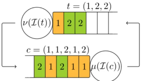
2 1 2 1 1 c = (1, 1, 2, 1, 2) µ(I(c)) 1 2 2 t = (1, 2, 2) ν(I(t))
Figure 6: A closed tandem network of two OI queues associated with the server pool of Figure 1. At most `1 = `2 = 4 jobs can be assigned to each class. The state is (c, t), with
c = (1, 1, 2, 1, 2) and t = (1, 2, 2). The corresponding aggregate state is that of the network of Figure 5. An incoming job of type 1 would seize the available token in first position (of class 1), while an incoming job of type 2 would seize the available token in second position (of class 2).
Stationary distribution Assuming Si 6= Sj or Ki 6= Kj for each pair {i, j} ⊂ I of classes, the
Markov process defined by the detailed state (c, t) is irreducible. The proof is provided in the appendix. Known results on networks of quasi-reversible queues [11] then show that this process is quasi-reversible, with stationary distribution
π(c, t) = 1
GΦ(c)Λ(t), ∀c, t ∈ C : |c| + |t| = `,
where Φ is defined by the recursion (5) and the initial step Φ(∅) = 1, as in §2.3; similarly, Λ is defined recursively on C by Λ(∅) = 1 and
Λ(t) = 1
ν(I(t))Λ(t1, . . . , tm−1), ∀t ∈ C \ {∅}.
We go back to the aggregate state x giving the number of tokens of each class held by jobs in service. With a slight abuse of notation, we define its stationary distribution by
π(x) = X
c:|c|=x
X
t:|t|=`−x
π(c, t), ∀x ∈ X . (10)
As in §2.3, we can show that we have π(x) = 1
GΦ(x)Λ(` − x), ∀x ∈ X , where the functions Φ and Λ are defined on X by
Φ(x) = X
c:|c|=x
Φ(c) and Λ(y) = X
t:|t|=y
respectively. These functions Φ and Λ satisfy the recursions (2) and (8), respectively, with the initial conditions Φ(0) = Λ(0) = 1. Hence, the aggregate stationary distribution of the system state x is exactly that obtained in §3.2 by combining the randomized load balancing with balanced fairness.
Also, using the definition of Λ, we can rewrite (6) as follows: for each x ∈ X and i ∈ I(x),
φi(x) = X c:|c|=x 1 GΦ(c) P t:|t|=`−xΛ(t) 1 GΦ(x)Λ(` − x) µi(c), = X c:|c|=x X t:|t|=`−x π(c, t) π(x) µi(c).
Hence, the average per-class service rates are still as defined by balanced fairness. By symmetry, it follows that the average per-class arrival rates, ignoring the release order of tokens, are as defined by the randomized load balancing. Specifically, for each y ∈ X and i ∈ I(y), we have
λi(y) = X c:|c|=`−y X t:|t|=y π(c, t) π(` − y)νi(t),
where λi(y) is the arrival rate of jobs assigned to class i in state y under the randomized load
balancing, given by (7), and νi(t) denotes the rate at which the first available token of class i is
seized under the deterministic load balancing:
νi(t) = m X p=1 tp=i (ν(I(t1, . . . , tp)) − ν(I(t1, . . . , tp−1))).
As in §2.3, the stationary distribution of the system state is unchanged by the addition of random routing, as long as the average traffic intensity of each class remains constant. Hence we can again reach some approximate insensitivity to the job size distribution within each class by enforcing frequent job interruptions and resumptions.
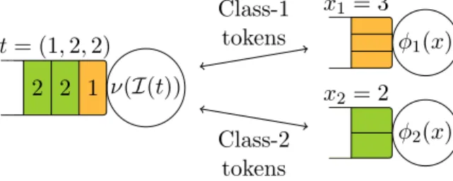
Application with balanced fairness As announced earlier, we can also combine our token-based load balancing algorithm with balanced fairness. The assignment of jobs to classes is still regulated by a single bucket containing available tokens, sorted in release order, but the resources are now allocated according to balanced fairness. The corresponding queueing model consists of an OI queue and a Whittle network, as represented in Figure 7.
2 2 1 t = (1, 2, 2) ν(I(t)) φ1(x) x1= 3 φ2(x) x2= 2 Class-1 tokens Class-2 tokens
Figure 7: A closed queueing system, consisting of an OI queue and a Whittle network, associated with the server pool of Figure 1. At most `1 = `2 = 4 jobs can be assigned to each
The intermediary state (x, t), retaining the release order of available tokens but not the arrival order of jobs, defines a Markov process. Its stationary distribution follows from known results on networks of quasi-reversible queues [11]:
π(x, t) = 1
GΦ(x)Λ(t), ∀x ∈ X , ∀t ∈ C : x + |t| = `.
We can show as before that the average per-class arrival rates, ignoring the release order of tokens, are as defined by the dynamic load balancing of §3.2.
The insensitivity of balanced fairness to the job size distribution within each class is again preserved. The proof of [6] for Cox distributions extends directly. Note that this does no imply that performance is insensitive to the job size distribution within each type. Indeed, if two job types with different size distributions can be assigned to the same class, then the distribution of the job sizes within this class may be correlated to the system state upon their arrival. This point will be assessed by simulation in Section 4.
Observe that our token-based mechanism can be applied to balance the load between the queues of an arbitrary Whittle network, as represented in Figure 7, independently of the system considered. Examples or such systems are given in [5].
4 Numerical results
We finally consider two examples that give insights on the performance of our token-based algorithm. We especially make a comparison with the static load balancing of Section 2 and assess the insensitivity to the job size distribution within each type. We refer the reader to [10] for a large-scale analysis in homogeneous pools with a single job type, along with a comparison with other (non-insensitive) standard policies.
Performance metrics for Poisson arrival processes and exponentially distributed sizes with unit mean follow from (9). By insensitivity, these also give the performance when job sizes within each class are i.i.d., as long as the traffic intensity is unchanged. We resort to simulations to evaluate performance when the job size distribution is type-dependent.
Performance is measured by the job blocking probability and the resource occupancy. For each k = 1, . . . , K, we let βk = 1 G X x≤`: xi=`i, ∀i∈I:k∈Ki Φ(x)Λ(` − x)
denote the probability that a job of type k is blocked upon arrival. The equality follows from PASTA property [14]. Symmetrically, for each s = 1, . . . , S, we let
ψs= 1 G X x≤`: xi=0, ∀i∈I:s∈Si Φ(x)Λ(` − x)
denote the probability that server s is idle. These quantities are related by the conservation equation K X k=1 νk(1 − βk) = S X s=1 µs(1 − ψs). (11)
We define respectively the average blocking probability and the average resource occupancy by β = PK k=1νkβk PK k=1νk and η = PS s=1µs(1 − ψs) PS s=1µs .
There is a simple relation between β and η. Indeed, if we let ρ = (PK
k=1νk)/(PSs=1µs) denote
the total load in the system, then we can rewrite (11) as ρ(1 − β) = η.
As expected, minimizing the average blocking probability is equivalent to maximizing the average resource occupancy. It is however convenient to look at both metrics in parallel. As we will see, when the system is underloaded, jobs are almost never blocked and it is easier to describe the (almost linear) evolution of the resource occupancy. On the contrary, when the system is overloaded, resources tend to be maximally occupied and it is more interesting to focus on the blocking probability.
Observe that any stable server pool satisfies the conservation equation (11). In particular, the average blocking probability β in a stable system cannot be less than 1 −1ρ when ρ > 1. A similar argument applied to each job type imposes that
βk≥ max 0, 1 − 1 νk X s∈S i:k∈KiSi µs , (12) for each k = 1, . . . , K.
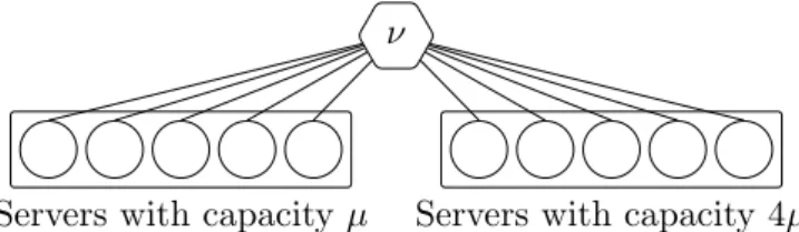
4.1 A single job type
We first consider a pool of S = 10 servers with a single type of jobs (K = 1), as shown in Figure 8. Each class identifies a unique server and each job can be assigned to any class. Half of the servers have a unit capacity µ and the other half have capacity 4µ. Each server has ` = 6 tokens and applies PS policy to its jobs. We do not look at the insensitivity to the job size distribution in this case, as there is a single job type.
Servers with capacity µ Servers with capacity 4µ ν
Figure 8: A server pool with a single job type. Classes are omitted because each of them corresponds to a single server.
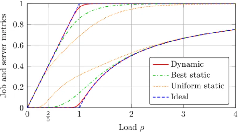
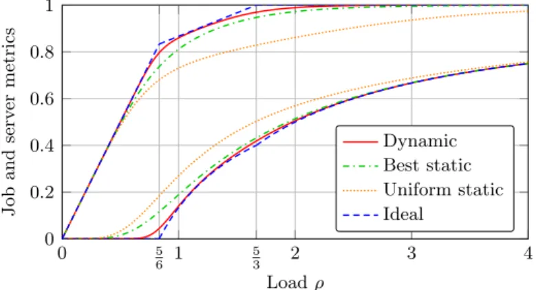
Comparison We compare the performance of our algorithm with that of the static load bal-ancing of Section 2, where each job is assigned to a server at random, independently of system state, and blocked if its assigned server is already full. We consider two variants, best static and uniform static, where the assignment probabilities are proportional to the server capacities and uniform, respectively. Ideal refers to the lowest average blocking probability that complies with the system stability. According to (11), it is 0 when ρ ≤ 1 and 1 −1ρ when ρ > 1. One can think of it as the performance in an ideal server pool where resources would be constantly optimally utilized. The results are shown in Figure 9.
0 2 5 1 2 3 4 0 0.2 0.4 0.6 0.8 1 Load ρ Job and serv er metrics Dynamic Best static Uniform static Ideal
Figure 9: Performance of the dynamic load balancing in the pool of Figure 8. Average blocking probability (bottom plot) and resource occupancy (top plot).
The performance gain of our algorithm compared to the static policies is maximal near the critical load ρ = 1, which is also the area where the delta with ideal is maximal. Elsewhere, all load balancing policies have a comparable performance. Our intuition is as follows: when the system is underloaded, servers are often available and the blocking probability is low anyway; when the system is overloaded, resources are congested and the blocking probability is high whichever scheme is utilized. Observe that the performance under uniform static deteriorates faster, even when ρ < 1, because the servers with the lowest capacity, concentrating half of the arrivals with only 15-th of the service capacity, are congested whenever ρ > 25. This stresses the need for accurate rate estimations under a static load balancing.
Asymptotics when the number of tokens increases We now focus on the impact of the number of tokens on the performance of the dynamic load balancing. A direct calculation shows that the average blocking probability decreases with the number ` of tokens per server, and tends to ideal as ` → +∞. Intuitively, having many tokens gives a long run feedback on the server loads without blocking arrivals more than necessary (to preserve stability). The results are shown in Figure 10.
0 0.2 0.4 0.6 0.8 1 1.2 1.4 1.6 0 0.1 0.2 0.3 0.4 Load ρ Blo cking prob abilit y 1 token 2 tokens 3 tokens 6 tokens 10 tokens Ideal
Figure 10: Impact of the number of tokens on the average blocking probability under the dy-namic load balancing in the pool of Figure 8.
is obtained with small values of ` and the performance is already close to the optimal with ` = 10 tokens per server. Hence, we can reach a low blocking probability even when the number of tokens is limited, for instance to guarantee a minimum service rate per job or respect multitasking constraints on the servers.
4.2 Several job types
We now consider a pool of S = 6 servers, all with the same unit capacity µ, as shown in Figure 11. As before, there is no parallel processing. Each class identifies a unique server that applies PS policy to its jobs and has ` = 6 tokens. There are two job types with different arrival rates and compatibilities. Type-1 jobs have a unit arrival rate ν and can be assigned to any of the first four servers. Type-2 jobs arrive at rate 4ν and can be assigned to any of the last four servers. Thus only two servers can be accessed by both types. Note that heterogeneity now lies in the job arrival rates and not in the server capacities.
ν 4ν
Servers with capacity µ Figure 11: A server pool with two job types.
Comparison We again consider two variants of the static load balancing: best static, in which the assignment probabilities are chosen so as to homogenize the arrival rates at the servers as far as possible, and uniform static, in which the assignment probabilities are uniform. Note that best static assumes that the arrival rates of the job types are known, while uniform static does not. As before, ideal refers to the lowest average blocking probability that complies with the system stability. The results are shown in Figure 12.
Regardless of the policy, the slope of the resource occupancy breaks down near the critical load ρ = 56. The reason is that the last four servers support at least 45-th of the arrivals with only 23-rd of the service capacity, so that their effective load is 65ρ. It follows from (12) that the average blocking probability in a stable system cannot be less than 45(1 −56ρ1) when ρ ≥ 56.
0 5 6 1 5 3 2 3 4 0 0.2 0.4 0.6 0.8 1 Load ρ Job and serv er metrics Dynamic Best static Uniform static Ideal
Figure 12: Performance of the dynamic load balancing in the pool of Figure 11. Average block-ing probability (bottom plot) and resource occupancy (top plot).
Under ideal, the slope of the resource occupancy breaks down again at ρ = 53. This is the point where the first two servers cannot support the load of type-1 jobs by themselves anymore.
Otherwise, most of the observations of §4.1 are still valid. The performance gain of the dynamic load balancing compared to best static is maximal near the first critical load ρ = 56. Its delta with ideal is maximal near ρ = 56 and ρ = 53. Elsewhere, all schemes have a similar performance, except for uniform static that deteriorates faster.
Overall, these numerical results show that our dynamic load balancing algorithm often out-performs best static and is close to ideal. The configurations (not shown here) where it was not the case involved very small pools, with job arrival rates and compatibilities opposite to the server capacities. Our intuition is that our algorithm performs better when the pool size or the number of tokens allow for some diversity in the assignments.
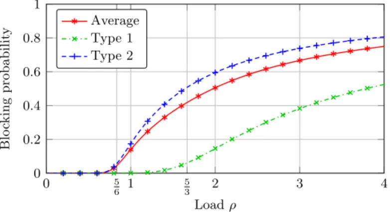
(In)sensitivity We finally evaluate the sensitivity of our algorithm to the job size distribution within each type. Figure 13 shows the results. Lines give the performance when job sizes are exponentially distributed with unit mean, as before. Marks, obtained by simulation, give the performance when the job size distribution within each type is hyperexponential: 13-rd of type-1 jobs have an exponentially distributed size with mean 2 and the other 23-rd have an exponentially distributed size with mean 12; similarly, 16-th of type-2 jobs have an exponentially distributed size with mean 5 and the other 56-th have an exponentially distributed size with mean 15. 0 5 6 1 5 3 2 3 4 0 0.2 0.4 0.6 0.8 1 Load ρ Blo cking pro babilit y Average Type 1 Type 2
Figure 13: Blocking probability under the dynamic load balancing in the server pool of Fig-ure 11, with either exponentially distributed job sizes (line plots) or hyperexpo-nentially distributed sizes (marks). Each simulation point is the average of 100 independent runs, each built up of 106 jumps after a warm-up period of 106 jumps. The corresponding 95% confidence interval, not shown on the figure, does not exceed ±0.001 around the point.
The similarity of the exact and simulation results suggests that insensitivity is preserved even when the job size distribution is type-dependent. Further evaluations, involving other job size distributions, would be necessary to conclude.
Also observe that the blocking probability of type-1 jobs increases near the load ρ = 53, which is twice less than the upper bound ρ = 103 given by (12). This suggests that the dynamic load balancing compensates the overload of type-2 jobs by rejecting more jobs of type 1.
5 Conclusion
We have introduced a new server pool model that explicitly distinguishes the compatibilities of a job from its actual assignment by the load balancer. Expressing the results of [5] in this new model has allowed us to see the problem of load balancing in a new light. We have derived a deterministic, token-based implementation of a dynamic load balancing that preserves the insensitivity of balanced fairness to the job size distribution within each class. Numerical results have assessed the performance of this algorithm.
For the future works, we would like to evaluate the performance of our algorithm in broader classes of server pools. We are also interested in proving its insensitivity to the job size distri-bution within each type.
References
[1] I. Adan and G. Weiss. A loss system with skill-based servers under assign to longest idle server policy. Probability in the Engineering and Informational Sciences, 26(3):307321, 2012.
[2] L. A. Barroso, J. Clidaras, and U. H¨olzle. The Datacenter As a Computer: An Introduction to the Design of Warehouse-Scale Machines. Morgan & Claypool Publishers, 2nd edition, 2013.
[3] S. A. Berezner and A. E. Krzesinski. Order independent loss queues. Queueing Systems, 23(1-4):331–335, Mar. 1996.
[4] T. Bonald and C. Comte. Balanced fair resource sharing in computer clusters. Performance Evaluation, 116(Supplement C):70–83, Nov. 2017.
[5] T. Bonald, M. Jonckheere, and A. Prouti`ere. Insensitive load balancing. SIGMETRICS Perform. Eval. Rev., 32(1):367–377, June 2004.
[6] T. Bonald and A. Prouti`ere. Insensitivity in processor-sharing networks. Performance Evaluation, 49(1):193–209, Sept. 2002.
[7] T. Bonald and A. Prouti`ere. Insensitive bandwidth sharing in data networks. Queueing Syst., 44(1):69–100, 2003.
[8] S. Fujishige. Submodular Functions and Optimization, Volume 58 - 2nd Edition. Elsevier Science, July 2005.
[9] K. Gardner, S. Zbarsky, S. Doroudi, M. Harchol-Balter, and E. Hyytia. Reducing latency via redundant requests: Exact analysis. SIGMETRICS Perform. Eval. Rev., 43(1):347–360, June 2015.
[10] M. Jonckheere and B. J. Prabhu. Asymptotics of insensitive load balancing and blocking phases. SIGMETRICS Perform. Eval. Rev., 44(1):311–322, June 2016.
[11] F. P. Kelly. Reversibility and Stochastic Networks. Cambridge University Press, New York, NY, USA, 2011.
[12] A. E. Krzesinski. Order independent queues. In R. J. Boucherie and N. M. van Dijk, editors, Queueing Networks: A Fundamental Approach, pages 85–120. Springer US, Boston, MA, 2011.
[13] Y. Lu, Q. Xie, G. Kliot, A. Geller, J. R. Larus, and A. Greenberg. Join-Idle-Queue: A novel load balancing algorithm for dynamically scalable web services. Performance Evaluation, 68(11):1056–1071, Nov. 2011.
[14] R. Serfozo. Introduction to Stochastic Networks. Stochastic Modelling and Applied Prob-ability. Springer New York, 1999.
[15] V. Shah and G. de Veciana. High-Performance Centralized Content Delivery Infrastructure: Models and Asymptotics. IEEE/ACM Transactions on Networking, 23(5):1674–1687, Oct. 2015.
[16] M. van der Boor, S. Borst, and J. van Leeuwaarden. Load balancing in large-scale systems with multiple dispatchers. In Proceedings of INFOCOM 2017, 2017.
Appendix: Proof of the irreducibility
We prove the irreducibility of the Markov process defined by the state (c, t) of a tandem network of two OI queues, as described in §3.3. Throughout the proof, we will simply refer to such a network as a tandem network, implicitly meaning that it is as described in §3.3.
Assumptions We first recall and name the two main assumptions that we use in the proof. • Positive service rate. For each i ∈ I, Ki6= ∅ and Si 6= ∅.
• Separability. For each pair {i, j} ⊂ I, either Si 6= Sj or Ki 6= Kj (or both).
Result statement The Markov process defined by the state of the tandem network is irre-ducible on the state space S = {(c, t) ∈ C2: |c| + |t| = `} comprising all states with `i tokens of
class i, for each i ∈ I.
Outline of the proof We provide a constructive proof that exhibits a series of transitions leading from any feasible state to any feasible state with a nonzero probability. We first describe two types of transitions and specify the states where they can occur with a nonzero probability. • Circular shift : service completion of a token at the head of a queue. This transition is always possible thanks to the positive service rate assumption. Consequently, states that are circular shifts of each other can communicate. We will therefore focus on ordering tokens relative to each other, keeping in mind that we can eventually apply circular shifts to move them in the correct queue.
• Overtaking: service completion of a token that is in second position of a queue, before its predecessor completes service. Such a transition has the effect of swapping the order of these two tokens. By reindexing classes if necessary, we can work on the assumption that class-i tokens can overtake the tokens of classes 1 to i − 1 in (at least) one of the two queues, for each i = 2, . . . , N . The proof of this statement relies on the separability assumption.
1 2 3 4
µ1 µ2 µ3
ν1 ν2 Job types
Job classes
Servers
Figure 14: A technically interesting toy configuration. We have K2 = K3 and S3 ( S2, so that
class-2 tokens can overtake class-3 tokens in the queue of tokens held by jobs in service but not in the queue of available tokens. On the other hand, K1 ( K2 and
S1 = S2, so that class-2 tokens can overtake class-1 tokens in the queue of available
tokens but not in the queue of tokens held by jobs in service. In none of the queues can class-2 tokens overtake tokens of classes 1 and 3 at once.
It is tempting to consider more sophisticated transitions, for instance where a token overtakes several other tokens at once. Unfortunately, our assumptions do not guarantee that such tran-sitions can occur with a nonzero probability. An example is shown in Figure 14. The two operations circular shift and overtaking will prove to be sufficient. We first combine them to show the following intermediary result:
• From any feasible state, we can reach the state where all class-N tokens are gathered at some selected position in one of the two queues while the position of the other tokens is unchanged.
We finally prove the irreducibility result by induction on the number N of classes. As announced, the proof is constructive: it gives a series of transitions leading from any state to any other state. The induction step can be decomposed in two parts:
• By repeatedly moving class-N tokens at a position where they do not prevent other tokens from overtaking each other, we can order the tokens of classes 1 to N −1 as if class-N tokens were absent. The induction assumption ensures that we can perform this reordering. • Once the tokens of classes 1 to N − 1 are well ordered, class-N tokens can be positioned
among them.
We now detail the steps of the proof one after the other.
Circular shift Because of the positive service rate assumption, a token at the head of either of the two queues has a nonzero probability of completing service and moving to the end of the other queue. We refer to such a transition as a circular shift.
Now let (c, t) ∈ S and (c0, t0) ∈ S, with c = (c1, . . . , cn), t = (t1, . . . , tm), c0 = (c01, . . . , c0n0)
and t0= (t01, . . . , t0m0). Assume that the sequence (c1, . . . , cn, t1, . . . , tm) is a circular shift of the
sequence (c01, . . . , c0n0, t10, . . . , t0m0). Then we can reach state (c0, t0) from state (c, t) by applying
many circular shifts if necessary. An example is shown in Figure 15 for the configuration of Figure 14. All states that are circular shifts of each other can therefore communicate.
Overtaking We say that a token in second position of one of the two queues overtakes its predecessor if it completes service first. Such a transition allows us to exchange the positions of these two tokens, therefore escaping circular shifts to access other states.
1 2 c = (1, 2) µ(I(c)) 4 1 2 3 2 4 t = (4, 1, 2, 3, 2, 4) ν(I(t))
(a) Initial state
1 2 4 2 3 c = (3, 2, 4, 1, 2) µ(I(c)) 4 1 2 t = (4, 1, 2) ν(I(t)) (b) Final state
Figure 15: Circular shift. Sequence of transitions to reach state (b) from state (a): all tokens complete service in the first queue; all tokens before that of class 3 complete service in the second queue; the first two tokens complete service in the first queue.
Can such a transition occur with a nonzero probability? It depends on the classes of the tokens in second and first positions, denoted by i and j respectively. The token in second position can overtake its predecessor if it receives a nonzero service rate. In the queue of tokens held by jobs in service, this means that there is at least one server that can process class-i jobs but not class-j jobs, that is Si * Sj. In the queue of available tokens, this means that there is
at least one job type that can seize class-i tokens but not class-j tokens, that is Ki * Kj. Since
states that are circular shifts of each other can communicate, the queue where the overtaking actually occurs does not matter.
The separability assumption ensures that, for each pair of classes, the tokens of at least one of the two classes can overtake the tokens of the other class, in at least one of the two queues. We now show a stronger result: by reindexing classes if necessary, we can work on the assumption that class-i tokens can overtake the tokens of classes 1 to i − 1 in at least one of the two queues (possibly not the same), for each i = 2, . . . , N .
We first use the inclusion relation on the power set of {1, . . . , K} to order the type sets Ki
for i ∈ I. Specifically, we consider a topological ordering of these sets induced by their Hasse diagram, so that a given type set is not a subset of any type set with a lower index. An example is shown in Figure 16a. The tokens of a class with a given type set can thus overtake (in the first queue) the tokens of all classes with a lower type set index. Only classes with the same type set are not dissociated.
Symmetrically, we use the inclusion relation on the power set of {1, . . . , S} to order the server sets Si for i ∈ I. We consider a topological ordering of these sets induced by their Hasse
diagram, so that a given server set is not a subset of any server set with a lower index, as illustrated in Figure 16b. The tokens of a class with a given server set can thus overtake (in the second queue) the tokens of all classes with a lower server set index. Thanks to the separability assumption, if two classes are not dissociated by their type sets, then they are dissociated by their server sets.
This allows us to define a permutation of the classes as follows: first, we order classes by increasing type set order, and then, we order the classes that have the same type set by increasing server set order. The separability assumption ensures that all classes are eventually sorted. The tokens of a given class can overtake the tokens of all classes with a lower index, either in the queue of available tokens or in the queue of tokens held by jobs in service (or both).
∅ {1} K1 {2} K4 {1, 2} K2= K3
(a) Hasse diagram of the type sets. (K1 = {1},
K4 = {2}, K2 = K3 = {1, 2}) is a possible topological ordering. ∅ {1} {2} S3 {3} S4 {1, 2} S1 = S2 {1, 3} {2, 3} {1, 2, 3}
(b) Hasse diagram of the server sets. (S3 = {2},
S4= {3}, S1 = S2 = {1, 2}) is a possible
topo-logical ordering.
Figure 16: A possible ordering of the classes of Figure 14 is 1, 4, 3, 2.
Moving class-N tokens Using the two operations circular shift and overtaking, we show that, from any given state, we can reach the state where all class-N tokens are gathered at some selected position in one of the two queues, while the position of the other tokens is unchanged. We proceed by moving class-N tokens one after the other, starting with the token that is closest to the destination (in number of tokens to overtake) and finishing with the one that is furthest. Consider the class-N token that is closest to the destination but not well positioned yet (if any). This token can move to the destination by overtaking its predecessors one after the other. Indeed, the token that precedes our class-N token has a class between 1 and N − 1, so that our class-N token can overtake it in (at least) one of the two queues. By applying many circular shifts if necessary, we can reach the state where this overtaking can occur. Once this state is reached, our class-N token can then overtake its predecessor, therefore arriving one step closer to the destination. We reiterate this operation until our class-N token is well positioned.
For example, consider the state of Figure 15a and assume that we want to move all tokens of class 2 between the two tokens of classes 1 and 3 that are closest to each other. One of the class-2 tokens is already in the correct position. Let us consider the next class-2 token, initially positioned between tokens of classes 3 and 4. We first apply circular shifts to reach the state depicted in Figure 15b. In this state, there is a nonzero probability that our class-2 token overtakes the class-3 token, which would bring our class-2 token directly in the correct position. Proof by induction We finally prove the stated irreducibility result by induction on the number N of classes. For N = 1, applying circular shifts is enough to show the irreducibility because all tokens are exchangeable. We now give the induction step.
Let N > 1. Assume that the Markov process defined by the state of any tandem network with N − 1 classes that satisfies the positive service rate and separability assumptions is irreducible. Now consider a tandem network with N classes that also satisfies these assumptions. We have shown that, starting from any feasible state, we can move class-N tokens at a position where they do not prevent other tokens from overtaking each other. In particular, to reach a state from another one, we can first focus on ordering the tokens of classes 1 and N − 1, as if class-N tokens were absent. This is equivalent to ordering tokens in a tandem network with N − 1 classes that satisfies the positive service rate and separability assumptions. This reordering is feasible by the induction assumption. Once it is performed, we can move class-N tokens in a correct position, by applying the same type of transitions as in the previous paragraph.