Distributed computation of vector clocks in Petri nets unfolding for test selection

HAL Id: hal-01735406

https://hal.inria.fr/hal-01735406

Submitted on 15 Mar 2018

HAL is a multi-disciplinary open access

archive for the deposit and dissemination of

sci-entific research documents, whether they are

pub-lished or not. The documents may come from

teaching and research institutions in France or

abroad, or from public or private research centers.

L’archive ouverte pluridisciplinaire HAL, est

destinée au dépôt et à la diffusion de documents

scientifiques de niveau recherche, publiés ou non,

émanant des établissements d’enseignement et de

recherche français ou étrangers, des laboratoires

publics ou privés.

Distributed computation of vector clocks in Petri nets

unfolding for test selection

Loïg Jezequel, Agnes Madalinski, Stefan Schwoon

To cite this version:

Loïg Jezequel, Agnes Madalinski, Stefan Schwoon. Distributed computation of vector clocks in Petri

nets unfolding for test selection. Workshop on Discrete Event Systems (WODES), May 2018, Sorrento,

Italy. �hal-01735406�

Distributed computation of vector clocks in

Petri nets unfolding for test selection

Lo¨ıg Jezequel1, Agnes Madalinski2, and Stefan Schwoon3

1

Universit´e de Nantes, LS2N, UMR CNRS 6004, France (e-mail: [email protected])

2

Chair of Software Engineering, OvGU Magdeburg, Germany (e-mail: [email protected])

3

LSV (CNRS & ENS Cachan), Univ. Paris-Saclay & Inria, France (e-mail: [email protected])

Abstract. It has been shown that annotating Petri net unfoldings with time stamps allows for building distributed testers for distributed sys-tems. However, the construction of the annotated unfolding of a dis-tributed system currently remains a centralized task. In this paper we extend a distributed unfolding technique in order to annotate the result-ing unfoldresult-ing with time stamps. This allows for distributed construction of distributed testers for distributed systems.

1

Introduction

The co-ioco framework proposed in [7] introduced partial-order semantics to the well-known ioco theory of [11]. In both cases, inputs and outputs (or their absence) of the implementation are compared to those of the specification. How-ever, in the co-ioco setting, traces, inputs, and outputs are considered as partial orders, where actions specified as concurrent need to be implemented as such. This is of essential importance for distributed systems where concurrency cap-tures the physical distribution of the components of the system.

Test architectures for distributed systems can be classified into two types: global testers that have control over the entire system under test, and distributed testers where several single and concurrent testers are controlling the compo-nents of the system under test. In [7, 1] it is shown how, starting from a system specified as a Petri net or a network of automata, a global tester can be con-structed using Petri net unfoldings and SAT. Additionally, [8] show that if the unfolding procedure is extended with time stamps, the resulting global tester can be transformed into a distributed one. However, the computation of the global tester is still centralized and constructs (a prefix of) the unfolding of the entire system.

In this work we provide a novel framework for constructing single testers (to-gether constituting a distributed tester) containing the time-stamp information necessary to test global conformance. These testers are computed in a distributed way. This work is grounded on the results of [9] and [3], extending them with

timed information. Our timed information is logical : it counts occurences of ac-tions. This is similar to vector clocks in distributed systems, cf. [6, 5, 10].

This paper is organized as follows. In Section 2 we provide a running example. In Section 3, we give the basic notations for our formal model. The notion of Petri-net unfolding and its link to testers are defined in Section 4. After that, we recall distributed Petri-net unfolding in Section 5, and we extend these to incorporate time stamps in Section 6. Finally, we show how to build interface summaries with time stamps, which are central for distributed unfoldings, in Section 7.

The main contribution of this paper is the method we propose for computing time stamps during distributed unfolding (described in Section 6 and at the end of Section 7). Unlike [8], our approach avoids the expensive operation of unfolding the entire system, working on individual components instead. This also allows to unify the results of [9] and [3] in order to build a distributed algorithm for unfolding Petri nets.

2

Running example

As a running example, we shall use the Petri net depicted in Figure 2, showing the interaction of a consumer (in the middle) with two producers (left and right). For various purposes, we will use two different decompositions of it:

1. into the five subnets indicated in Figure 2, where A, C are the producers, B is the consumer, and X, Y are the interfaces between the consumer and the left (respectively right) producer;

2. into three (overlapping) components A, B, C, where A consists of producer A with its interface X, C consists of producer C with its interface Y , and B consists of consumer B with both interfaces.

Notice that each place and transition belongs to exactly one subnet. The places and transitions of the interfaces belong to exactly two components, and the others belong to exactly one.

Intuitively, producer A offers some product that it can create from certain

base materials. Each of these materials may be available (places p0, q0, r0) or not

(p, q, r). Interface X acts as an agent handling the interaction between A and B. This agent, upon receiving an order from the consumer B, registers a demand for the product with A. Depending on the availability of the base materials, the product can be either delivered to the consumer, or one of the sides decides to cancel the transaction. Producer C works in a similar fashion, using different

base materials (places s, t and s0, t0) and communicating through interface Y .

Finally, B can be thought of as a customer wishing to perform certain actions x, y, or z. For x and z only one of the producers is needed, whereas for y both are required.

A X B Y C p q r p 0 q 0 r 0 iA _dA _sA A1 A2 a1 a2 or der A stop A deliver A b1 b2 _b3 _b4 _b5 b6 _b7 _b8 _b9 x 0 y 0 z 0 ret ry A retry C x y z b10 b11 b12 b13 t s t 0 s 0 iC _dC _sC C1 C2 c1 c2 c3 c4 _c5 or der C demand C stop C supply C de cline C deliver C Fig. 1. An example with one consumer B and tw o pro ducers A, C connected b y in terfaces X , Y .

3

Distributed systems modeling

We now formalize the framework exemplified above: compound systems rep-resented as labelled Petri nets. We fix an alphabet Σ of labels and a set of components C.

A Petri net is a tuple pn = hP, T, F, M0, `, γi where P and T are two disjoint

sets of nodes called places and transitions, respectively, F ⊆ P × T ∪ T × P

is a flow relation, M0 ⊆ P is an initial marking, ` : (P ∪ T ) → Σ associates

labels to nodes, and γ : (P ∪ T ) → 2C_{associates each node with a subset of the}

components. The elements of F are called the arcs.

For consistency, we require that for all p ∈ P , t ∈ T , hp, ti ∈ F or ht, pi ∈ F implies γ(p) ⊆ γ(t), i.e. a transition can only interact with places of its own components. Moreover, every component c ∈ C has at least one initially marked

place, i.e. there exists p ∈ M0 with c ∈ γ(p).

Example. Figure 2 shows an example of a Petri net. Places are represented as circles (with black tokens for the initial marking), transitions as rectangles, and the flow relation as arrows. Labels are shown next to the nodes, and C = {A, B, C}, corresponding to A, B, C from Section 2, where nodes in X belong to both A and B, those in Y to both B and C, and all others to exactly one of A, B, C.

A marking is a set of places. A transition t is said to be firable from marking

M ⊆ P iff•t = { p | (p, t) ∈ F } ⊆ M . In this case the firing of t leads to the new

marking (M \•t) ∪ t•, where t•= { p | (t, p) ∈ F }. A marking M is reachable in

pn if and only if there exists a sequence of transition firings leading from M0 to

M .

Notice that our definition of marking and our semantics of firing are simplified with respect to the standard definitions; this is justified by the fact that we deal with safe nets only, where for any reachable marking M and any transition t,

•_{t ⊆ M implies M ∩ (t}•_\•_{t) = ∅.}

Projections and interfaces. Let C0⊆ C. The projection of pn to C0_{is the net}

π_C0(pn) = hP0, T0, F0, M₀0, `0, γ0i that preserves only nodes from C0, i.e. P0⊆ P ,

T0 ⊆ T , and x ∈ P0 _{∪ T}0

iff γ(x) ∩ C0 6= ∅; moreover, F0_{, M}0

0, `0, γ0 are the

respective restrictions of F, M0, `, γ to P0∪ T0. Note that γ0 is still a mapping to

C, not just to C0. Abusing notation, we shall write πc for π{c} when c ∈ C. For

instance, when pn is the net in Figure 2, we obtain A = πA(pn), B = πB(pn),

and C = πC(pn). With this in mind, we also call A, B, C “components” when

there is no confusion.

For two components c, c0 _{∈ C, the interface of pn between c and c}0 is

πc(πc0(pn)) = π_c0(π_c(pn)). For instance, the interface of A, B in Figure 2 is

the subnet X, and Y is the interface of B, C. A net is said to contain a gateway to component c if it contains nodes that belong to c but none that belong to c

alone. For instance, A = πA(pn) contains a gateway to B (which is exactly the

The interaction graph of pn is the undirected graph whose nodes are the

elements of C, and where {c, c0} is an edge iff c and c0_{have a non-empty interface.}

A net is tree-like if its interaction graph is a tree.

An automaton is a Petri net such that for any transition t one has |•t| =

|t•_{| = 1, and where M}

0 is a singleton. For instance, the net in Figure 3 obeys

this condition.

Timed nets. Finally, in certain cases we will wish to include (logical) timing information in Petri nets. A vector clock is a mapping from C to N. In practice, vector clocks shall count how many events have fired per component. A timed net is a pair pn = hpn, θi, equipping a Petri net pn with a clock mapping θ that associates a vector clock to each transition of pn. The projection of pn

to C0 ⊆ C is πC0(pn) := hπC0(pn) , θ0i, where θ0 is the restriction of θ to the

nodes of π_C0(pn). Note that this operation retains vector clock information for

all components in C, including components outside C0.

4

Petri nets unfolding and test

The unfolding of a Petri net pn is another, acyclic Petri net un(pn) that describes the complete behaviour of pn: all reachable markings and all partial orders of transition firings are preserved. The unfolding of a Petri net in fact enumerates the partial orders of transition firings of pn, merged on common prefixes. In general, the unfolding is an infinite structure, but our algorithms only consider finite prefixes of it. As shown in [8], adding well-chosen time stamps to the unfolding of a Petri net allows to build a distributed tester for the compound system modeled by the original net – simply by projecting a finite prefix of the unfolding onto each component.

In this section, we formally define unfoldings. We then show how time stamps should be added to an unfolding.

Unfoldings are usually formalized from the notion of branching process. A

branching process of a Petri net pn = hP, T, F, M0, `, γi is a Petri net pn0 =

hQ, E, F0_{, M}0

0, `0, γ0i (where places are usually called conditions, and transitions

are usually called events) associated with a function λ : Q∪E → P ∪T . (Abusing

notation, we naturally extend λ to sets.) Assuming M0= {p0, . . . , pk}, the finite

branching processes of pn are defined inductively as follows:

– The net with conditions q0, . . . , qk so that λ(q0) = p0, . . . , λ(qk) = pk, no

events, and initial marking {q0, . . . , qk} is a branching process of pn.

– Let pn0_{be a branching process of pn where for some reachable marking M of}

pn0, λ(M ) makes some transition t of pn firable. Let M0 be the subset of M

such that λ(M0) =•t. If pn0has no event e with λ(e) = t such that•e = M0,

then the net obtained by adding to pn0 a new event e with λ(e) = t, a new

condition for every place p of t• labelled by p, new arcs from each condition

of M0 to e and from e to each new condition, is also a branching process of

– For all nodes x, `0(x) = `(λ(x)) and γ0(x) = γ(λ(x)).

The set of all branching processes of a Petri net pn, finite and infinite, is defined by closing the finite branching processes under countable unions (see [2]). In particular, the union of all finite branching processes is called the unfolding of pn, denoted un(pn).

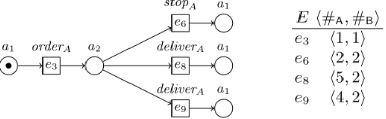
Example. Consider Figure 2 (left). It depicts a finite branching process of the net from Figure 2 restricted to component A, i.e. producer A and its interface X. The labelling λ is given next to the conditions and events.

p q iA a1 r e1 e2 e3 orderA e4 p0 _q0 r0 dA a2 e5 A1 stopA e6 e7 A2 p q sA iA a1 sA r e8 deliverA e9 deliverA iA a1 iA a1

E h#

, #

i

e

h1, 0i

e

h1, 0i

e

h1, 1i

e

h1, 0i

e

h4, 1i

e

h2, 2i

e

h3, 1i

e

h5, 2i

e

h4, 2i

Fig. 2. A branching process of πA(pn), where pn is the net from Figure 2, and

associ-ated time stamps.

Given two nodes x, y of a branching process, we say that: x is a causal pre-decessor of y, denoted x < y, if there exists a non-empty path of arcs from x to y. By x ≤ y we mean x < y or x = y, and if x ≤ y or y ≤ x we say that x and y are causally related. The nodes x and y are in conflict if there exists a condition c (different from x and y) so that one can reach both x and y from c via two paths that start with different arcs. The nodes x and y are concurrent if they are neither causally related nor in conflict.

Given an event e of a branching process, we define its configuration, noted

[e], as the set of its causal predecessors events: [e] = {e0| e0 _{≤ e}.}

A timed branching process of pn is the pair hpn0, θi, where pn0 is a branching

process of pn, and θ(e)(c) is the number of events e0 satisfying e0 ≤ e and

c ∈ γ0(e0). In this case, θ is also called a collection of time stamps. We denote

un(pn) as the timed unfolding of pn.

Example. Consider again Figure 2, and recall that nodes of the interface X

belong to both A and B. The column marked #A provides the value θ(e)(A) for

In the following, we consider projections of timed or untimed unfoldings to

components C0 ⊆ C. In this context, notice that πC0(un(pn)) is not the same

as un(π_C0(pn)); the latter contains vector clock information from transitions in

π_C0(pn) alone, while the former has it for all of pn.

Example. Figure 3 shows the projection of the timed branching process from Figure 2 to B. Only the conditions of X and the events in which it participates are preserved. a1 e3 orderA a2 e6 stop_A a1 e8 deliverA e9 deliverA a1 a1

E h#

, #

i

e

h1, 1i

e

h2, 2i

e

h5, 2i

e

h4, 2i

Fig. 3. Projection of Figure 2 to component B.

5

Distributed unfolding

In this section, we review a distributed algorithm for computing (a prefix of) the unfolding of a net without time stamps. There exists a straightforward, cen-tralized algorithm for this task, which applies the inductive characterization of a branching processes, adding one event at a time (see [2]). The result is easily equipped with time stamps, and it is known ([8]) how to use a finite unfolding prefix to produce distributed testers. However, the intermediate unfolding prefix can be much larger than those testers.

We are interested by the approach of [9], which computes unfolding prefixes component by component. In this section, we briefly describe a slightly general-ized version of this algorithm (the original algorithm computes complete prefixes whereas testers are built on arbitrary prefixes). This method uses smaller un-folding prefixes, but adding time stamps is not straightforward. Starting from Section 6, we show how to close this gap.

Let pn = hP, T, F, M0, `, γi be a compound system represented as a Petri net.

In order to perform distributed unfolding, we impose the following restrictions: 1. pn is tree-like.

2. Every (non-empty) interface in pn is an automaton.

The first assumption is required by the distributed unfolding approach of [9], which can be slightly weakened (see [4]). Notice that this implies |γ(x)| ≤ 2 for any node x. The second restriction comes from our solution to distributed unfoldings with timing information, based on [3].

Example. Consider again Figure 2. This decomposition respects our restric-tions: the interfaces X and Y are automata, and B communicates with A and C.

Let c, c0 ∈ C be two components. A {c, c0_{}-automaton is an automaton in}

which γ(x) = {c, c0} for all nodes x. According to our restriction, every

non-empty interface X in pn is a {c, c0}-automaton (for some c, c0_{). If moreover X is}

a gateway to c0, we call it a (c, c0)-gateway.

Let A be a tree-like net with a (c, c0_{)-gateway X. Then we denote C[A, X] ⊆}

C the set of all components having at least one node in A, except c0. Let B be

another tree-like net with a (c0, c)-gateway Y such that {c, c0} is the only edge

appearing in the interaction graphs of both A and B. Then we say that A, B

meet at {c, c0}. Notice that in this case, C[A, X] and C[B, Y ] are disjoint.

Distributed unfoldings rely on two basic operations: the projection π_C0,

allow-ing to extract components from compound systems, and a composition operation

k. The latter will allow us to replace an interface X between components c and c0

by another {c, c0}-automaton (which, in general, will be a behavioural refinement

of X). Thus, let A, B be tree-like nets meeting at {c, c0}, with X a (c, c0_)-gateway

of A and Y a (c0, c)-gateway of B. We present their composition in three steps:

1. building the synchronous product Z of X and Y , 2. replacing X and Y by Z, and

3. merging A and B on Z.

We formalize these notions below. In a more general setting this composition would be the synchronous product of A and B. We present it this way to facilitate intuition on the distributed unfolding approach. For notational simplicity, we shall assume that the sets of places, transitions etc of A, B, X, Y, Z are indexed

with the name of the net, and denote with NA, NB etc the sets of nodes (i.e.

places and transitions) of A, B etc.

Synchronous product. The synchronous product of {c, c0}-automata X and

Y is the {c, c0}-automaton X k Y = hP, T, F, M0, `, γi with

– P = PX× PY and M0= M0,X× M0,Y,

– T = { ht1, t2i ∈ TX× TY | `X(t1) = `Y(t2) },

– F = { hhx1, x2i, hx01, x02ii ∈ P × T ∪ T × P | (x1, x01) ∈ FX∧ (x2, x02) ∈ FY },

– `(ht1, t2i) = `X(t1) = `Y(t2), and γ(ht1, t2i) = {c, c0}.

Replacement. Let A have a (c, c0)-gateway X and Z = X k Y for some Y .

The replacement of X by Z is A[X/Z] := hP0, T0, F0, M₀0, `0, γ0i, where, with

N_A00 := NA\ NX:

– P0 = (PA\ PX) ∪ PZ and T_A0 = (TA\ TX) ∪ TZ;

– F0 = (FA∩ NA00× NA00) ∪ FZ

∪ { hn, hnA, nBii ∈ N_A00× NZ | hn, nAi ∈ FA}

– M₀0 = (M0,A\ M0,X) ∪ M0,Z;

– for all n ∈ N_A00, `0(n) = `A(n) and γ0(n) = γA(n);

– for all n ∈ NZ, `0(n) = `Z(n) and γ0(n) = {c, c0}.

The definition for the case where Z = Y k X is analogous.

Merging. Consider two tree-like nets A, B meeting at {c, c0} such that Z is

equally a (c, c0)-gateway in A and a (c0, c)-gateway in B. The merging of A and

B on Z is the net hP, T, F, M0, `, γi with:

– P = PA∪ PB; T = TA∪ TB; F = FA∪ FB;

– M0= M0,A∪ M0,B;

– `(n) = `A(n) for n ∈ NA\ NZ, `(n) = `B(n) for n ∈ NB\ NZ, and `(n) =

`Z(n) for n ∈ NZ;

– γ(n) = γA(n) for n ∈ NA\ NZ, γ(n) = γB(n) for n ∈ NB\ NZ, and

γ(n) = {c, c0} for n ∈ NZ.

Notice that this definition of step (3) relies on the fact that Z is exactly the same in A and B, so in particular the places and transitions have the same names. Moreover, it is easy to see that the resulting net is also tree-like.

Finally, from the above three steps, we can define the composition operation for compound systems: For A, B, X, Y and Z = X k Y as above, we denote the composition of A and B as the merging of A[X/Z] and B[Y /Z] on Z.

Distributed unfolding. From now on, for simplicity of presentation, we shall consider a compound system pn with three components A, B, C, giving rise to projections A, B, C. We assume that A and B interact through interface X, while B and C interact through interface Y . Hence pn = A k B k C. As described in [9], all the results given below for these three components extend directly to compound systems with tree-shaped interaction graphs.

The distributed unfolding of [9] is based on the following factorability prop-erties:

un(pn) = un(A) k un(B) k un(C), (1)

= πA(un(pn)) k πB(un(pn)) k πC(un(pn)) . (2)

The approach of [9] consists in computing the factors πA(un(pn)), πB(un(pn)),

and πC(un(pn)) by local computations only, that is, without computing un(pn).

These computations are strongly independent and thus can be distributed. One can remark that these factors, are exactly forming a distributed tester, provided that one can add correct time stamps to them.

The idea for distributed computing of the unfolding factors comes from the recursive application of equation (1) in (2):

πA(un(pn)) = πA(un(A) k un(B) k un(C))

= un(A) k πA(un(B) k un(C))

This lets one compute πA(un(pn)) by propagating information from C to A:

First C computes πB(un(C)) and sends it to B, which can use this to compute

πA(un(B) k πB(un(C))) and send it to A. Then A is able to compute πA(un(pn)).

A similar reasoning can be applied to the two other components: πC(un(pn)) =

un(πC(un(πB(un(A)) k B)) k C), and πB(un(pn)) = un(πB(un(A)) k B k un(C)).

This approach is not yet constructive: in order to compute one unfolding factor, one requires the unfolding of other components, which are in general infinite. Thus, we wish to replace them by a finite object describing all the possible behaviours of the interface of this system. We call such an object an interface summary.

Consider a net A having a gateway X to some component c. An interface

summary of A with respect to X is any automaton sumX(A) = hP, T, F, M0, `, γi

satisying the following: there exists a sequence of transition firings t1. . . tk

start-ing from M0 with label sequence w = `(t1) . . . `(tk) if and only if there exists a

sequence of transition firings t0

1. . . t0k in πc(un(A)) starting from its initial state

and having the same label sequence w. Notice that this implies, in particular,

that all nodes of sumX(A) belong to c.

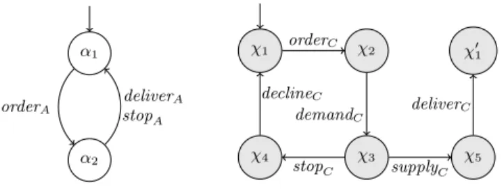
Example. Consider the component A (consisting of the subnets A and X) of the net in Figure 2. An interface summary of A w.r.t. X is shown in Figure 4 (left). Moreover, an interface summary of component B w.r.t. the interface Y is shown in Figure 4 (right). Notice that the first summary is identical to X (when the latter is viewed as an automaton), whereas the second has a terminating

behaviour; this is because, while Y is cyclic, B terminates after deliverC.

α1 α2 orderA deliverA stopA χ1 χ2 χ3 χ4 χ5 χ01 orderC stopC supplyC declineC demandC deliverC

Fig. 4. Summary of A w.r.t. its interface X (left); summary of B w.r.t. Y (right).

Interface summaries can then replace unfoldings and projections in the above equations, leading to a new information propagation process:

πA(un(pn)) = un(A k πA(un(B k πB(un(C)))))

= un(A k sumX(B k sumY(C)))

πB(un(pn)) = un(sumX(A) k B k sumY(C))

Example. We illustrate the computation of πC(un(pn)) using the net from

Figure 2. As mentioned in the previous example, sumX(A) is identical to X

itself, therefore, in our example, sumX(A)kB is the same as B. In turn, sumY(B)

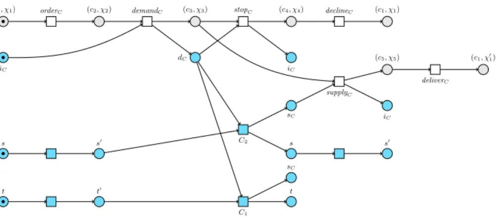
is shown in Figure 4 (right). The result of unfolding the composition of this summary with C is shown in Figure 5, where places representing the summary are shown in grey.

(c1, χ1) (c2, χ2) (c3, χ3) (c4, χ4) (c1, χ1) (c5, χ5) (c1, χ01) iC dC iC sC iC sC s s0 _{s s}0 t t0 _t

orderC demandC stopC declineC

supplyC

deliverC

C2

C1

Fig. 5. Unfolding of the composition of C with the summary of B w.r.t. Y .

Notice that, for instance, the above computation of πC(un(pn)) finally

un-folds some composition of C with summaries of X and Y . However, the latter do not contain any timing information on components A and B. Thus, this method cannot be directly used to compute a distributed tester for co-ioco conformance because the latter requires timing information for all components. In the remain-der of the paper, we show how to tackle this problem.

6

Distributed time stamps computation

We now study how to incorporate timing information into distributed unfoldings. The distributed approach from Section 5 relies on unfolding one single compo-nent, composed with a summary of other components. However, one action in a summary may represent multiple actions in several components. For instance,

in the summary of A from Figure 4 (left), the action deliverA requires multiple

transition firings in A (cf Figure 2 and Figure 3). A natural way out of this dilemma is to consider the unfolding of timed nets whose vector clocks convey the missing information. In this sense, vector clocks represent time increments. Let pn = hpn, θi be a timed net. A timed branching process of pn is a pair

hpn0_{, θ}0_{i, where pn}0 _{is a branching process of pn, and for all events e, θ}0_{(e)(c) =}

P

e0_∈[e]θ(λ(e0))(c). We denote un(pn) as the timed unfolding of pn. Notice that

unfolding of hpn, θ1i, where θ1(t)(c) = 1 if c ∈ λ(t) and 0 otherwise. We therefore

denote pn₁:= hpn, θ1i.

In the rest of this section, we revisit the material from Section 5 and extend it with timed information. This results in a distributed method for computing distributed testers, subject to finding appropriate summaries. This final problem is then solved in Section 7.

Timed merging. Consider two timed nets hA, θAi and hB, θBi meeting at

{c, c0_{}, where A has a (c, c}0_{)-gateway X, and B has a (c}0_{, c)-gateway Y . Then}

hA, θAi k hB, θBi = hA k B, θi, where for every transition t of A k B, we have the

following:

– if t = (ta, tb) is a transition of X k Y , then θ(t)(c) = θA(ta)(c) for c ∈ C[A, X]

and θ(t)(c) = θB(tb)(c) for other components c;

– otherwise, θ(t) = θA(t) (resp. θB(t)) if t is a transition of A (resp. B).

Timed summaries. To make the distributed approach practical, a notion of

timed interface summary is also necessary. Consider a timed net hA, θAi with

gateway X to some component c. A timed interface summary of A w.r.t. X is

any timed net sumX(A) = hsumX(A) , θXi such that sumX(A) is an interface

summary of A w.r.t. X, and for any c0 ∈ C[A, X] and any path t1. . . tn with

label sequence w in sumX(A),P

n

i=1θX(ti)(c0) is the minimal number of

tran-sitions from c0 among all sequences of transitions in A whose labels contain w

as a subsequence. Notice that the sequence achieving the minimum for some

component c0 is not necessarily the same as for another component c00.

α1 α2

orderAh1, 1i

stopAh1, 1i

deliverAh3, 1i

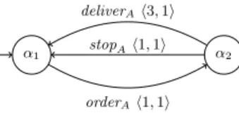
Fig. 6. Timed interface summary of A w.r.t. interface X.

Example. Consider the component A of the net in Figure 2 and its interface

X. Figure 6 shows a timed summary of A1 w.r.t. X, where actions are

an-notated with time increments over A and B. This summary can be seen as a transformation of the projection shown in Figure 3, where conditions mapped

to a1 are fused together4. Time increments correspond to the differences in the

time stamps between e6, e8, e9, respectively, and e3 in Figure 3. Since the two

occurrences of deliverA in Figure 3 correspond to different time increments, a

4

minimum has to be taken to obtain the time increment of deliverA in Figure 6.

Over A the minimum of 3 (obtained from e8) and 4 (obtained from e9) gives 3.

Similarly, over B the minimum of 1 and 1 gives 1.

By making use of this extension of k and of timed summaries, we can extend the distributed unfolding algorithm of Section 5 to build distributed testers. This is expressed (in the case of a three components) in the following theorem, which is the first part of our contribution.

Theorem 1. If summaries with time increments exist, then the propagation equations hold:

πA(un(pn)) = un(A1k sumX(B1k sumY(C1)))

πB(un(pn)) = un(sumX(A1) k B1k sumY(C1))

πC(un(pn)) = un(sumY(sumX(A1) k B1) k C1)

Proof (Sketch of the proof ). We consider the particular case of A. The principle of the proof would be similar for any component in our particular example, as well as for any component in a more complex system, provided its interaction graph is a tree.

The statement clearly holds for the untimed aspects, that is, considering only the sequences of transition firing that are possible. Indeed, the structure of the summaries as well as the definition of the product is exactly the same than in the case without time. The proof of [9] can thus be used. This also allows

to identify all the elements (and in particular, the events) of πA(un(pn)) and

un(A k sumX(B k sumY(C))), except the time stamps. Let us denote by θπ the

time stamps from πA(un(pn)) and by θU the time stamps in the timed unfolding

un(A1k sumX(B1k sumY(C1))). Consider an event e from these two objects and

a component c. Looking at how θπ is computed one gets

θπ(e)(c) =

X

e0_∈[e]

θ1(λ(e0))(c)

where θ1are the clock vectors of pn1(this is a direct application of the definition

of the branching processes and the definition of the projection). Looking at how

θU is computed one gets

θU(e)(c) =

X

e0_∈[e]

θA(λ(e0))(c) + θX(λ(e0))(c)

where θA gives the time increments in A1 and θX gives the time increments in

sumX(B1k sumY(C1)). The proof in fact mainly consists in linking θX to θB

and θC, the time increments in B1 and C1 respectively. Indeed, for any event e

corresponding to a transition t from X, by definition of timed summaries, one gets that

X

e0_∈[e]

if c ∈ C[A, X], and that otherwise P

e0_∈[e]θX(λ(e0))(c) is the total number of

transitions to be fired before e in c. This allows to identify θU(e)(c) (as a sum of

θA, θB, and θC) and θπ(e)(c) (in terms of θ1, which is itself a sum of the three

same time increments).

A complete proof would have a closer look at θU, using the explicit

con-struction of the summaries described below. These summaries are indeed com-puted from unfoldings, allowing to identify any event of un(pn) to an event in

un(A1k sumX(B1k sumY(C1))) as above. This event would itself be identified

to a couple of events from the unfolding of A1 and that of B1k sumY(C1). In

turn, this couple would be identified to a triple of events in the unfolding of A1,

B1, and C1. Linking the time stamps/increments of these different events would

allow to conclude, with similar reasoning as the one drawn in the sketch of the proof of Theorem 2 below.

7

Interface summary construction

We now provide the missing part of the puzzle by presenting a method for computing timed summaries. This allows to effectively construct the distributed unfoldings mentioned in Theorem 1. Our method is a modification of the – untimed – summary construction from [3], which we recall in Section 7.1. We then explain how to deal with time increments in Section 7.2.

7.1 Summary construction without time increments

Consider a net A having a (c, c0)-gateway X. We recall how to construct an

interface summary of A with respect to X from a finite prefix of un(A). To this end, we first introduce some notations.

Let pn0 be a branching process of A. An event (condition) n of pn0 is is

an X-event (X-condition) if γ(n) = {c, c0}. Let e be any event of pn0_{. We}

note M (e) the unique set of conditions marked after firing all events in [e] and

St(e) = { λ(b) | b ∈ M (e) } the places of A associated with M (e). We note M (e)X

the unique X-condition in M (e). Since by assumption X is an automaton, such a condition always exists. We note Xp(e) the set of X-predecessors of e, that is the

X-events among the causal predecessors of e: Xp(e) = { e0∈ [e] | γ(e0_{) = {c, c}0_{} }.}

Event e0 is a strong cause of e, denoted e0  e, if e0 _{< e and b}0 _{< b for every}

b ∈ M (e) \ M (e0), b0∈ M (e0_{) \ M (e).}

Algorithm 1 describes the construction of the interface summary in two steps. The first step (lines 1 to 10) computes a prefix of un(A) containing sufficient in-formation to construct a summary, which is produced by the second step (lines 11 to 14).

The first step relies on two notions: cut-off events (after which the unfolding contains no additional information useful for us) and cut-off candidates (where we provisionally stop unfolding but may resume later on). We define both using the notations of the algorithm:

An event e is a cut-off of pn0 if it is an X-event and pn0 already contains a

non-cut-off X-event e0 (called companion of e) such that St(e) = St(e0).

Let Xcopn0(e) denote the set of non cut-off X-events of pn0concurrent with e.

Then event e is a cut-off candidate of pn0if it is not an X-event and pn0contains

e0  e such that St(e) = St(e0_{), Xp(e}0_{) = Xp(e), and Xco}

pn0(e) ⊆ Xco_pn0(e0).

Finally, we say that event e frees ec if ec is a cut-off candidate of pn0 before the

addition of e but not after its addition.

Algorithm 1 Summary of a net A with interface X

1: let pn0 be the branching process of A with no events 2: let co = ∅ and coc = ∅

3: While Ext(pn0, co, coc) 6= ∅ do

4: choose an event e in Ext(pn0, co, coc) 5: If e is a cut-off event then let co = co ∪ {e} 6: Elseif e is a cut-off candidate of pn0then 7: let coc = coc ∪ {e}

8: Else for every e0∈ coc do

9: If e frees e0 then coc = coc \ {e0} 10: extend pn0with e

11: let aut := πc0(pn0)

12: For every e ∈ co with companion e0do 13: fuse M (e)X with M (e0)X in aut

14: Return aut

In the first step of Algorithm 1, Ext(pn0, co, coc) denotes possible extensions

of pn0 that are not causal successors of events in co ∪ coc. The choice of e in this

set has to be done carefully, respecting a well chosen order (see [2] for example).

The second step of Algorithm 1 first extracts the interface portion of pn0

by projecting onto c0 (this suffices because X is a gateway). Moreover, since

by assumption X is an automaton, and because of the properties of branching

processes, πc0(pn0) is an acyclic finite automaton. In fact, each terminal node

of πc0(pn) is an X-condition b such that the unique event e ∈ •b is a cut-off.

The cut-off condition ensures that b0:= M (e0)X, where e0 is the companion of e,

satisfies λ(b0) = λ(b), and, since St(e) = St(e0), b and b0 have the same future:

isomorphic structures would be built from M (e) and M (e0) if the unfolding

process was never stopped. This justifies fusing b and b0 _{as one single place in}

lines 12 and 13.

7.2 Adding time increments

Now, let hA, θAi be a timed net with A having gateway X as in Section 7.1. We

shall produce a timed interface summary of A w.r.t. X by applying the following modification to Algorithm 1:

The unfolding step (lines 1 to 10) and the fusion of conditions (lines 12 and 13) remain unchanged. However, it does not suffice to simply annotate each

event e in aut with the time increment given by θA(λ(e)): to obtain the correct

time stamp for e, one would have to sum all the time increments from [e] in pn0.

This use of time increments rather than time stamps allows one to build correct timed interface summaries.

Thus, to compute the time increments θX, we have to take into account the

events in pn0 outside X that were removed by the projection. Notice that each

X-event e can be associated to a unique minimal set Req(e) of non X-events that have to fire in order to enable e. This set is constituted of all predecessors of e that are not X-predecessors of e, nor predecessors of X-predecessors of e. In other words, it consists of all the events that have to occur between the closest X-predecessor of e and e itself. The time increment associated to e is then:

∀c, θX(e)(c) = θA(λ(e))(c) +

X

e0_∈Req(e)

θA(λ(e0))(c).

Moreover, if the fusion of two conditions in line 13 results in two or more au-tomata transitions having the same (singleton) preset, label, and postset, these transitions are fused into one single transition whose time increment is the point-wise minimum of the time increments of the fused transitions.

Example. For Figure 2, the timed summary of A w.r.t. X produced by this procedure is the one shown in Figure 6.

Theorem 2. The tuple haut, θXi, as computed by the above modification of

Al-gorithm 1, is a timed interface summary of hA, θAi.

Proof (Sketch of the proof ). The correctness of the summary without time in-crements is due to the use of the construction algorithm from [3].

We now discuss the correctness of the time-increment computation. We illus-trate it using the particular case of our running example, when computing the

timed summary of B0 := B k sumY(C) w.r.t. X. However, the argument

gener-alizes to any interface summary computation on tree-like nets by noticing that removing any edge from a tree (here between A and B) separates it into two disjoint sub-trees (here A alone and B and C together).

The correctness of the time increments in the particular case of the summary

of B0 := B k sumY(C) in our running example comes from the fact that the

components in the sub-tree rooted at B can all be considered independently. Indeed, all the timing information about other components than B can only appear on transitions from the interfaces of B with its neighbours. Moreover, for any component C 6= B (interacting through interface Y ), timing information on C can only appear on Y -transitions. Since Y is an automaton, no two concurrent

actions in the unfolding of B0 can have non-zero timing information on C. Thus,

given an X-event e, the events e0 in Req(e) with θ(e0)(C) 6= 0 can be totally

ordered. Thus, they are always executed in sequence, which guarantees that they can be added without ambiguity.

From that, the validity of the interface summary construction in systems

interface summary computed by our algorithm, one has that P

tiθX(ti)(C) is the minimum number of transitions from C that have to be fired in order to fire

t1. . . tn in this order. This is the property that we want to achieve for the time

increments in each component.

Finally, the fact that the time increments are computed independently for each component guarantees the validity of our interface summary.

8

Conclusion

In this paper we have proposed a procedure for building a tester for distributed systems. This tester is distributed as it complies with the definition given in [8]. The novelty of our approach with respect to this work on concurrent conformance is that the construction of the tester is achieved as the result of a distributed pro-cess. The main interest of our approach is thus that it can avoid the construction of a prefix of the unfolding of the Petri net representation of the full distributed system under test. Instead, the Petri net representation of each component of the system is unfolded separately. This allows to perform the generally costly computation of unfolding prefixes on small nets. Moreover, such a distributed approach has another practical interest. By definition, it allows for building dis-tributed test suits for a disdis-tributed system, even without having a complete view of this system. It thus extends one of the interest of distributed testers (being able to test a system from local views of its components) to the construction process of the tester itself.

Our work on distributed computation of distributed testers heavily relies on previous theoretical works from the authors. However, the new theoretical contribution associated to it is not negligible. We believe that this theoretical contribution is of interest all by itself, for two reasons. First, it unifies the results from [9] and [3]. This makes the distributed unfolding technique of the former effective, by providing a concrete way to build the interface summaries. Second, and mainly, this theoretical contribution shows that, during the distributed un-folding process, the local unun-folding of any component A can be equipped with time stamps on its events. This information gives the minimum number of tran-sitions that must fire in the other components for any event of the unfolding of A to happen. In other words, this brings a notion of logical time to Petri nets unfolding in the context of distributed systems modeling. The additional computational cost for building and propagating these time stamps along the distributed unfolding procedure is relatively small with respect to the cost of building (a prefix of) the unfolding itself.

References

1. Athanasiou, K., Ponce de Le´on, H., Schwoon, S.: Test case generation for concur-rent systems using event structures. In: TAP. pp. 19–37 (2015)

2. Esparza, J., Heljanko, K.: Unfoldings – A Partial-Order Approach to Model Check-ing. Springer (2008)

3. Esparza, J., Jezequel, L., Schwoon, S.: Computation of summaries using net un-foldings. In: FSTTCS. pp. 225–236 (2013)

4. Fabre, E.: Bayesian Networks of Dynamic Systems. Habilitation, Universit´e Rennes 1 (June 2007)

5. Fidge, C.J.: Timestamps in message-passing systems that preserve the partial or-dering. Australian Computer Science Communications 10(1), 56–66 (1988) 6. Lamport, L.: Time, clocks, and the ordering of events in a distributed system.

Communications of the ACM 21(7), 558–565 (1978)

7. Ponce de Le´on, H., Haar, S., Longuet, D.: Unfolding-based test selection for con-current conformance. In: ICTSS. pp. 98–113 (2013)

8. Ponce de Le´on, H., Haar, S., Longuet, D.: Distributed testing of concurrent sys-tems: Vector clocks to the rescue. In: ICTAC. pp. 369–387 (2014)

9. Madalinski, A., Fabre, E.: Modular construction of finite and complete prefixes of Petri net unfoldings. Fundamenta Informaticae 95(1), 219–244 (2009)

10. Mattern, F.: Virtual time and global states of distributed systems. In: International Workshop on Parallel and Distributed Algorithms. pp. 215–226 (1988)

11. Tretmans, J.: Testing concurrent systems: A formal approach. In: CONCUR. pp. 46–65 (1999)